Towards Automated Cadastral Map Improvement: A Clustering Approach for Error Pattern Recognition

Abstract

Positional accuracy in cadastral data is fundamental for secure land tenure and efficient land administration. However, many land administration systems (LASs) experience difficulties to meet accuracy standards, particularly when data come from various sources or historical maps, leading to disruptions in land transactions. This study investigates the use of unsupervised clustering algorithms to identify and characterize systematic spatial error patterns in cadastral maps. We compare Fuzzy c-means (FCM), Density-Based Spatial Clustering of Applications with Noise (DBSCAN), and Gaussian Mixture Models (GMMs) in clustering error vectors using two different case studies from Greece, each with different error origins. The analysis revealed distinctly different error structures: a systematic rotational pattern surrounding a central random-error zone in the first, versus localized gross errors alongside regions of different discrepancies in the second. Algorithm performance was context-dependent: GMMs excelled, providing the most interpretable partitioning of multiple error levels, including gross errors; DBSCAN succeeded at isolating the dominant systematic error from noise. However, FCM struggled to capture the complex spatial nature of errors in both cases. Through the automated identification of problematic regions with different error characteristics, the proposed approach provides actionable insights for targeted, cost-effective cadastral renewal. This aligns with fit-for-purpose land administration principles, supporting progressive improvements towards more reliable cadastral data and offering a novel methodology applicable to other LASs facing similar challenges.

1. Introduction

Accurate geospatial data are fundamental to the efficient operation of modern cadastral systems, supporting secure land tenure [1], effective land administration [2,3], fair taxation [4], infrastructure development [5], and reliable land transactions. Globally, modernizing land administration systems (LASs) [6], and especially improving the positional accuracy of cadastral data, remain ongoing challenges. This effort is driven by the need to refine the geometric characteristics of spatial information, ensuring the accurate representation of legal land objects and property boundaries [7]. Beyond initial LAS formation, there also exists the need for cadastral data renewal (i.e., the process of updating, correcting, and enhancing existing cadastral data and maps). This renewal is necessary to meet accuracy standards, technological advancements, and societal needs [8,9,10], and may involve digitizing analog maps, correcting errors, updating land registry information, and integrating cadastral data with other spatial information systems [8].

Many countries have adopted cadastral data renewal as a national policy to address technical and legal issues arising from outdated or inaccurate cadastral data, as illustrated by the Turkish Land Registry and Cadastre Modernization Project (TKMP) [8]. Also, in Croatia, several projects and studies are related to the homogenization method, in the same context [11,12]. The complexity and quality of spatial data vary widely between countries, due to differences in historical development, economic resources, and organizational structures, which in turn shape the required renewal approaches [12]. Best practices in LAS management emphasize progressive improvement, where data quality is improved incrementally over time, allowing the systems to remain functional even in their early stages [13]. This method recognizes that cadastral data can exist at varying levels of encoding and accuracy, both spatially and temporally. This practice aligns with the concept of fit-for-purpose land administration (FFPLA), which proposes flexible, upgradable systems, designed to take into account local needs, resources, and land tenure types, with a focus on incremental improvement [14].

Traditional methods for enhancing positional accuracy in LASs, such as re-surveying or manual adjustments, are often costly and time-consuming. This has led the research community to explore computational correction methods that transform existing datasets using a set of homologous points (corresponding features identified in two datasets) from higher-accuracy sources [15,16,17,18]. On the other hand, automated techniques, particularly those utilizing Artificial Intelligence (AI) to minimize manual effort and improve efficiency, remain scarce, mainly in the area of vectorization [19,20].

Within AI methods, unsupervised learning algorithms uncover hidden structures in data without requiring predefined labels [21,22]. Clustering, a core unsupervised learning method [23], groups data points based on a similarity metric, such as the Euclidean distance, to uncover meaningful insights [24]. Numerous clustering methods are documented in the literature, and Oyewole and Thopil [25] provide a recent classification of these approaches. These techniques have been widely applied to spatial data analysis tasks, such as identifying patterns in geographic data, detecting hotspots, and grouping similar spatial objects [26,27,28,29].

In the context of the progressive improvement of an LAS, clustering can be applied to error vectors that represent discrepancies between recorded locations on the system and more accurate survey data. If these errors have a spatial structure (i.e., are not randomly distributed), clustering can identify distinct groups of points with similar error characteristics, potentially indicating systematic biases introduced during data acquirement or processing. The optimal number of clusters in unsupervised learning, which is, in general, initially unknown, is a major issue because different algorithms—or even a single algorithm with different parameters—may produce different clusters of data [30]. Hence, various methods have been developed for the estimation of the optimal number of clusters, which is often ambiguous, (e.g., the elbow method, silhouette analysis, and information criteria) [31,32,33].

The Greek National Cadastre (GNC), like many national cadastral systems, faces ongoing challenges related to positional accuracy. Its history is marked by a series of incomplete or unsuccessful attempts to establish a comprehensive LAS [34]. Currently, it is organized under Laws 2308/1995 [35] and 2664/1998 [36], covering 59% of the country [37]. Despite these efforts, significant positional inaccuracies exist, particularly in areas covered by GNC first-generation surveys (1995–1999). These early surveys, while aiming for a 1:1000 scale accuracy in urban areas and 1:5000 in rural areas, are suffering from various issues, including systematic errors: (a) arising from the integration of administrative acts, such as land redistributions; and (b) introduced during the creation and use of photogrammetric diagrams [38].

Consequently, landowners submitted objections at an average rate of 20% of the total records (reaching up to 60% in certain areas), far exceeding the internationally accepted rate of 3–5% [37]. These discrepancies have led to legal disputes, difficulties in land transactions, and a general lack of trust in the accuracy of cadastral data. In response, the Greek State introduced Article 19A into Law 2664/1998 in 2011, enabling the en masse redefinition of land parcel positions and boundaries to support the renewal of the GNC in problematic regions.

To address these challenges, the GNC is actively exploring and implementing innovative technological solutions. In a pioneering move, it has become the first public organization in Greece to utilize Artificial Intelligence (AI) not only as a chat-bot for information, but also for making administrative decisions, aiming to accelerate the legal review process of land-related contracts. This initiative demonstrates a commitment to use advanced technologies in order to improve the effectiveness of cadastral administration [39].

This study explores the use of unsupervised clustering techniques to automatically detect and analyze systematic error patterns, focusing on two different case studies from Ioannina and Kastoria, Greece, both regions from the first-generation GNC surveys, reported for positional inaccuracies from local surveyors, suspected to have different error origins and spatial patterns of these inaccuracies. This research has the following objectives: (a) to evaluate the performance of multiple clustering algorithms in the domain of spatial errors in cadastral maps; (b) to determine the optimal number of clusters for each algorithm using suitable model selection techniques; (c) to compare the performance of the algorithms using a combination of quantitative and qualitative visual assessments of the clustering results, both in the error and in the geographic space; and (d) to assess the potential of the best-performing clustering approach for generating correction models to guide automated LAS positional quality improvement.

To our knowledge, this is the first application of clustering algorithms to uncover systematic spatial errors in LAS data. Beyond simply identifying clusters, we interpret their meaning in relation to known cadastral processes and error sources, resulting in insights about data quality improvement strategies, following the philosophy of FFPLA, regarding incremental improvement, in the context of the GNC’s needs, and its commitment using advanced technologies.

2. Data and Methods

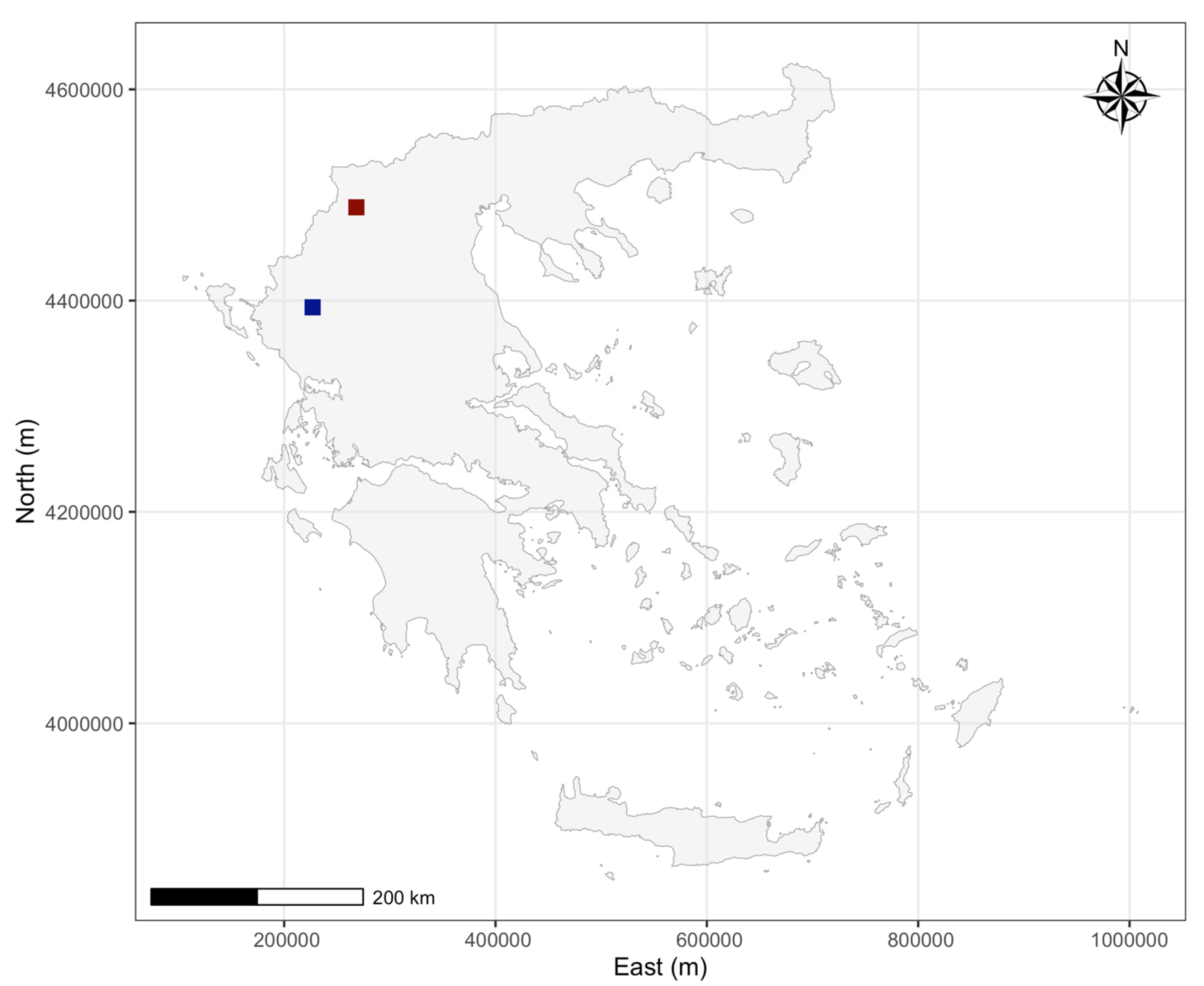
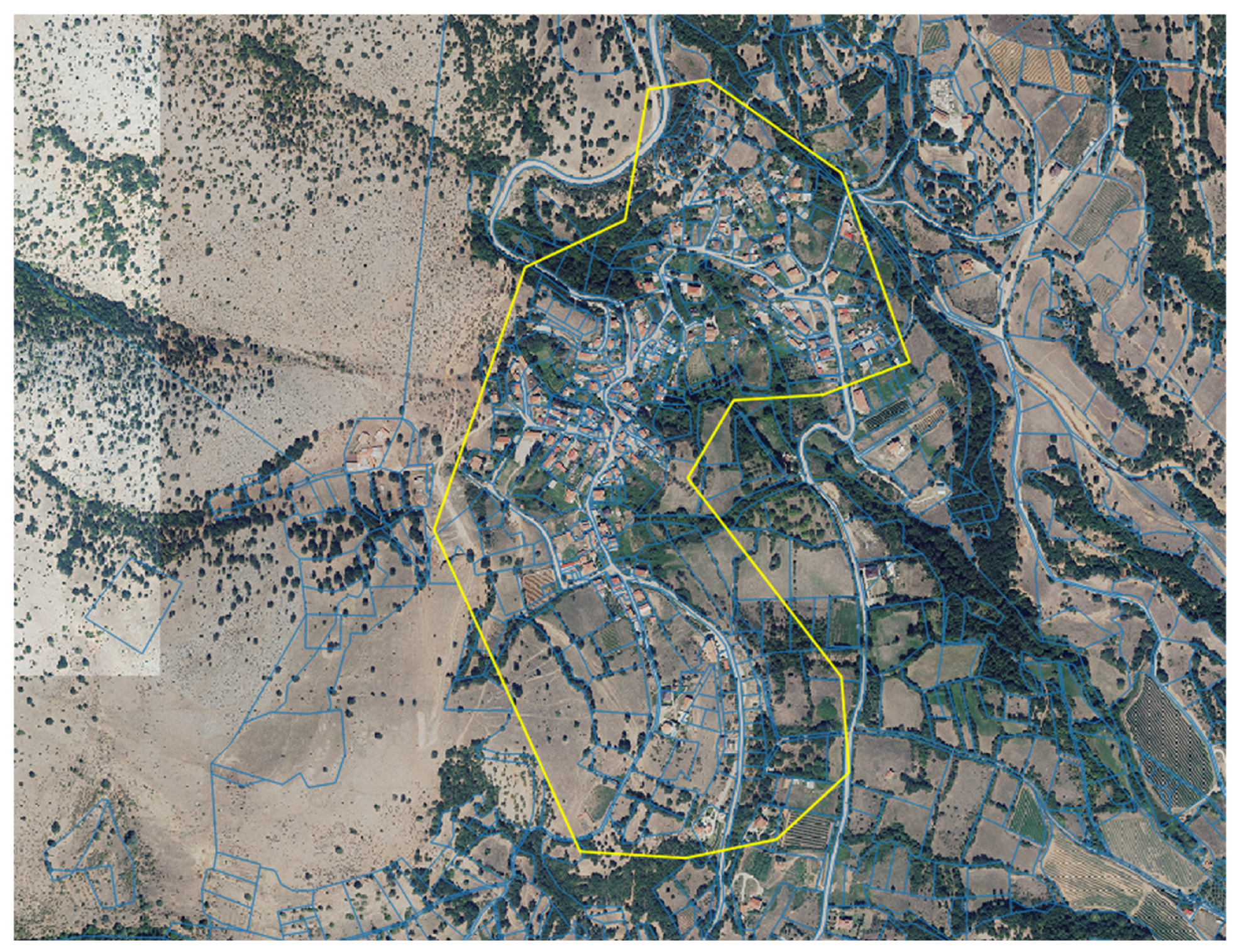
2.1. Study Area 1: Stavraki, Ioannina, Greece

The primary study area is located in Stavraki, a municipal unit within the Municipality of Ioannina, in the Region of Epirus, northwestern Greece (Figure 1). It spans approximately 7 square kilometers and has a mixed land use, predominantly residential areas combined with agricultural land and some commercial zones (Figure 2). Its topography consists of gently rolling hills, with an average elevation of 518 m above sea level. This area has been integrated into the GNC since 2005, and land records are managed by the operational cadastral office in Ioannina, responsible for maintaining property boundaries, ownership information, and related legal documentation. The cadastral municipality consists of 2541 cadastral parcels, representing individual land properties.

A key characteristic of the Stavraki area’s cadastral history is the enactment of an Implementing Act under the Greek Law 1337/1983 [40] in 2001. This Act aimed to reorganize and urbanize the land and create regularized parcels, addressing the municipality’s development needs. The Act involved (a) expropriation; (b) land contribution calculations; (c) the creation of new parcels; and (d) redistribution to the original owners. It is important to recognize that errors can be introduced at any stage of this complex Implementing Act process. The output of the Act was a map and reports that analytically define the final parcels using their Cartesian coordinates. This provided a precise, mathematical representation of the parcel boundaries in 2001, before the development of the cadastral map for the GNC in 2005.

Despite the precise analytical definition that was provided by the Implementing Act, the study area has known problems, with professional surveyors reporting that (a) the accuracy of the 2025 cadastral map does not meet the standards of the GNC and (b) the primary source of error is not within the Act itself, but rather in the subsequent integration process undertaken during the creation of the GNC geodatabase in 2005 [35]. These errors, introduced during the integration process, are the primary focus of this study area.

2.2. Study Area 2: Kefalari, Kastoria, Greece

To further assess the applicability of the clustering methodology across different cadastral contexts and error origins, a second study area, Kefalari, was included. Kefalari is a community within the Municipality of Kastoria in the Region of Macedonia, northern Greece (Figure 1). It spans approximately 1 square kilometer and is characterized by semi-rural land use (Figure 3). Its topography is predominantly mountainous, with an average elevation of 800 m above sea level. Kefalari has been integrated into the Hellenic Cadastre since 2008, and land records are managed by the operational cadastral office in Kastoria. This study area consists of 470 cadastral parcels and belongs to the cadastral municipality of Kastoria.

Kefalari has a different cadastral history. A Land Distribution Act was carried out by the Topographic Service of the Greek Ministry of Agriculture in 1978. These land distributions serve as vital historical archives across Greece, documenting land tenure rights and providing precise surveys and parcel subdivisions, particularly for agricultural land and rural settlements. Integrating these historical administrative acts into the modern GNC has not always been seamless, as already mentioned [38].

Specifically, in Kefalari, the local chapter of the Hellenic Association of Rural and Surveyor Engineers of Kastoria has reported significant technical errors during the integration through digitization and georeferencing of this historical Land Distribution Act map into the GNC database. This provides a different scenario for investigating the presence of gross errors compared to the primary study area, which displays more systematic discrepancies.

2.3. Data Sources

For the analysis, the following primary data sources are used:

• GNC Data: The current (2025) digital vector data of the GNC maps were obtained from its open data portal [41] in shapefile format for both study areas. These data are referenced to the Hellenic Geodetic Reference System 1987 (HGRS87) [42], the official coordinate system for surveying applications in Greece;
• Land Survey Study Data: Higher-accuracy data were obtained from the digital land surveying study that was conducted by the Municipality of Ioannina in 2001 at a scale of 1:500. The survey was referenced to the Greek western zone of the Transverse Mercator (TM3 western zone) [43]. The purpose of this survey was to be the base map for the Implementing Act.
• The 1978 Land Distribution diagrams of Kefalari, that were conducted by the Greek Ministry of Agriculture in 1978, at a scale of 1:1000, were scanned and georeferenced using rubber-sheeting with QGIS software (version 3.42) [44]. These maps were referenced to the old Greek Datum (GR-Datum, [42,43]). Subsequently, the entire set of 101 parcels of the 1978 diagram was digitized into shapefile format.

Figure 1. The two study areas’ location in Greece (with dark blue Stavraki and dark red Kefalari). Reference System: HGRS87 (Hellenic Geodetic Reference System 1987) [42].

Figure 1. The two study areas’ location in Greece (with dark blue Stavraki and dark red Kefalari). Reference System: HGRS87 (Hellenic Geodetic Reference System 1987) [42].

Figure 2. Orthophoto map of Stavraki (2015). The yellow area is the study area, and blue depicts the cadastral parcels.

Figure 2. Orthophoto map of Stavraki (2015). The yellow area is the study area, and blue depicts the cadastral parcels.

Figure 3. Orthophoto map of Kefalari (2015). The yellow area depicts the study area, and blue depicts the cadastral parcels.

Figure 3. Orthophoto map of Kefalari (2015). The yellow area depicts the study area, and blue depicts the cadastral parcels.

2.4. Data Preprocessing

The survey data and the land distribution diagram were transformed from the TM3 and GR-Datum to the HGRS87, respectively, using appropriate geodetic calculations [43] and the second degree polynomials method, as given by the Hellenic Mapping and Cadastral Organization for this purpose [45].

To determine positional errors, in both areas, homologous points were identified by a careful visual comparison of parcels, focusing on unambiguous parcel corners and boundary intersections, using the QGIS software [44]. This process ensured a one-to-one correspondence for each point used in the error vectors calculations, representing the same point of a parcel in both pairs of datasets, for the two study areas.

Coordinate differences were calculated as follows:

$$\begin{gathered} \Delta E_i=E_i-{E\prime }_i \\ \Delta N_i=N_i-{N\prime }_i \end{gathered}$$

(1)

where $\Delta E_i$ and Δ$N_i$ are the differences along the x and the y-axis, respectively, for a point $i$. In this form, the vector $[E_i,N_i]$ represents the coordinates from the 2025 digital cadastral map and $\left[{E\prime }_i,{N\prime }_i\right]$ from the digital 2001 land survey, both in HGRS87. The magnitude of the error vector (i.e., the length) was also calculated for every point $i$.

In Stavraki, homologous points in which the calculated error vector magnitude exceeded 1.5 m (initially a set of eight points) were excluded from the final analysis, resulting in a dataset of 500 points. This threshold was used to remove potential outliers or points with gross errors, focusing the analysis on systematic error patterns rather than isolated large inaccuracies. On the other hand, in Kefalari, due to the presence of gross errors, the entirety of the 400 identified homologous points were included in the analysis.

2.5. Clustering Algorithms

As already mentioned, clustering groups data points is based on a predefined similarity measure, without prior knowledge of the group labels. In this context, the goal is to group homologous points that have similar error values $(\Delta E, \Delta N)$, to reveal underlying spatial structure in the error distribution. If the errors were distributed randomly across the study areas, clustering would likely produce arbitrary groupings without meaningful interpretation. Nonetheless, we make the hypothesis that systematic errors will be expressed as spatially district patterns. All analyses was performed using the R language (version 4.4.2) [46] and the packages ‘cluster’ [47], ‘dbscan’ [48], ‘mclust’ [49], ‘factoextra’ [50], ‘ggplot2’ [51], and ‘sf’ [52].

2.5.1. Fuzzy c-Means

FCM is a clustering algorithm that extends the concept of ‘hard clustering’ (like k-means [53]) by allowing data points to belong to multiple clusters simultaneously, with varying degrees of membership [33]. This ‘fuzziness’ is particularly useful when cluster boundaries are not well-defined or when data points might have characteristics of multiple groups [54]. Initially developed by Dunn [55] and later improved by Bezdek [56], FCM aims to partition a dataset into k clusters by minimizing an objective function that considers both the distance of points to cluster centers and their membership degrees [57]. In the context of our cadastral error analysis, FCM offers a way to explore whether error patterns exhibit gradual transitions or overlapping characteristics, rather than strictly distinct, spatially separated groups. The core of FCM is the iterative minimization of the following objective function:

$$J_m=\sum _{i=1}^N\sum _{j=1}^k{\left(w_{ij}\right)}^m {‖x_i-c_j‖}^2$$

(2)

where $N$ is the number of data points (homologous points, in our case); $k$ is the predefined number of clusters; $w_{ij}$ is the membership degree of data point $x_i$ to cluster $c_j$ (a value between 0 and 1, where 1 represents full membership and 0 represents no membership); $m$ is the fuzzifier parameter (a real number greater than 1, controlling the level of fuzziness; typically, m = 2 [58], a value that was used in our study); $x_i$ is the i-th data point (the error vector $[\Delta E_i, \Delta N_i])$; $c_j$ is the centroid (mean vector) of cluster $j$; and $‖x_i-c_j‖$ is the Euclidean distance between data point $x_i$ and cluster centroid $c_j$.

The algorithm iteratively updates the membership values $w_{ij}$ and the cluster centroids $c_j$ until convergence. The membership update equation is as follows:

$$w_{ij}={\displaystyle \frac{1}{{\sum }_{\kappa =1}^k{\left({\displaystyle \frac{‖x_i-c_j‖}{‖x_i-c_{\kappa }‖}}\right)}^{\frac{2}{m-1}}}}$$

(3)

And the cluster centroid update equation is as follows:

$$c_j={\displaystyle \frac{{\sum }_{i=1}^n{w}_{ij}^m{x}_i}{{\sum }_{i=1}^n{w}_{ij}^m}}$$

(4)

The algorithm stops when either a maximum number of iterations is reached or the change in the objective function $J_m$ between successive iterations falls below a predefined threshold, indicating convergence.

An issue regarding the FCM algorithm is the initialization of the cluster centroids $c_j$ or the initial membership matrix ($W=w_{ij}$). As a result, FCM is susceptible to converging to a local optimum rather than the global optimum of the objective function $J_m$. Standard implementations in software often employ random initialization strategies, including randomly selecting k data points from the dataset as initial centroids, or randomly assigning initial membership values to each point for each cluster [59]. The clustering result corresponding to the run that achieves the minimum value of the objective function $J_m$ is then selected as the best solution among the runs performed [26,47].

The application of FCM to our cadastral error data involves using the error vectors $(\Delta E,\Delta N)$ as input $x_i$. The number of clusters, C, can be determined using the elbow method, examining the within-cluster sum of squares (WSS) [60]. The membership values and cluster centroids can then be visualized and analyzed to identify potential systematic error patterns. The algorithm was implemented using the ’fanny’ function from the cluster [47] package in R, which incorporates strategies to handle initialization and convergence.

2.5.2. Density-Based Spatial Clustering of Applications with Noise

DBSCAN is a clustering algorithm particularly well-suited for identifying clusters with an arbitrary shape and handling noise [61], making it a strong candidate to analyze cadastral error patterns. Unlike centroid-based methods, like FCM, DBSCAN does not assume that the clusters are spherical or elliptical [62]. Instead, it defines clusters based on the density of data points [63]. The algorithm operates on the basis that points within a cluster are densely packed together, while points belonging to different clusters, or noise points, are separated by regions of lower density. This density-based approach is suitable to our study because systematic errors in cadastral data may have spatial patterns that are linear or curved.

The DBSCAN algorithm is based on two key parameters [61,63]: (a) $\epsilon$, which defines the radius of a neighborhood around each data point; and (b) $minPts$, which specifies the minimum number of data points required within the radius $\epsilon$ for a point to be considered a ‘core point’. These parameters are used to define the $\epsilon$-neighborhood of a point $p$:

$$N_{\epsilon }\left(p\right)=\{q\in D:d\left(p,q)\right\}<\epsilon$$

(5)

where $D$ is the dataset of points and $d(p,q)$ is the Euclidean distance between points $p$ and $q$. A core point is one point $p$ if its $\epsilon$-neighborhood contains at least $minPts$ points:

$${|N}_{\epsilon }\left(p\right)|\ge minPts$$

(6)

A point $q$ is directly density-reachable from a point $p$ if $q$ is within the $\epsilon$-neighborhood of a point $p$, and $p$ is the core point:

$$q\in N_{\epsilon }\left(p\right) and{ |N}_{\epsilon }\left(p\right)|\ge minPts$$

(7)

A point $q$ is density-reachable from a point $p$ if there exists a chain of points $p_1,\dots ,p_n$ where $p_1=p$ and $p_n=q$, and each $p_{i+1}$ is directly density-reachable from $p_i$. Two points, $p$ and $q$, are density-connected if there exists a point $o$ such that both $p,q$ are density-reachable from $o$. A cluster is a set of density-connected points that is maximal with respect to density-reachability. Noise points are points that are not density-reachable from any other point. The algorithm proceeds iteratively, by examining each point and applying these definitions.

In our cadastral error analysis, the input data points to DBSCAN are the error vectors ($\Delta E,\Delta N)$. The $\epsilon$ parameter describes a distance in the error space, and $minPts$ represents the minimum number of points with similar error magnitudes and directions required to form a cluster. A suitable $\epsilon$ parameter can be selected using the k-nearest neighbor (kNN) distances for the dataset, represented as a matrix of points [63]. The kNN distance is defined as the distance from a point to its k-nearest neighbor (i.e., k, which corresponds to $minPts$) [61]. The algorithm was implemented using the ‘kNNdistplot’ and ‘dbscan’ functions from the ‘dbscan’ R package [48].

2.5.3. Gaussian Mixture Models

The GMM is a probabilistic model that assumes that data points are generated from a mixture of several Gaussian distributions [64]. It is a form of soft clustering, like FCM, assigning probabilities that a point belongs to each cluster [65].

The core concept of GMMs is to represent the overall probability density function (PDF) of the data as a weighted sum of individual Gaussian component densities. The PDF for a GMM with K components has parameters $\theta =(w_1,\dots ,w_K,{\mu }_1,\dots ,{\mu }_k, {\Sigma }_1,\dots ,{\Sigma }_k)$ and is given by the following [65,66,67]:

$$p\left(x\right)=\sum _{k=1}^G{w}_{\kappa }\mathcal{N}(x|{\mu }_{\kappa },{\Sigma }_{\kappa })$$

(8)

where $G$ is the number of Gaussian components (clusters), $x$ is the data point, $w_{\kappa }$ is the mixing coefficient for the k-th component, representing the prior probability of a data point belonging to that component ($0\le w_k\le 1$ and $\sum w_k=1$), and $\mathcal{N}\left(x\right|{\mu }_{\kappa },{\Sigma }_{\kappa })$ is the multivariate Gaussian probability density function for the k-th component, defined by the following:

$$\mathcal{N}\left(x \right|\mu ,\Sigma )={\displaystyle \frac{1}{\sqrt{\det \left(2\pi \Sigma \right)} }}{e}^{-1/2{\left(x-\mu \right)}^T{\Sigma }^{-1}(x-\mu )}$$

(9)

where $\mu$ is the vector of means, $\Sigma$ is the covariance matrix, $\mathrm{d}\mathrm{e}\mathrm{t}(.)$ is the determinant, and $T$ denotes the transpose.

The flexibility of GMMs comes from the parameterization of the covariance matrix ${\Sigma }_{\kappa }$, which determines the geometric properties of each Gaussian component k [65]. Specifically, the clusters are ellipsoidal, centered at the mean vector ${\mu }_{\kappa }$ with other geometric features, such as the volume, shape, and orientation, to be determined by the covariance matrix.

The GMM algorithm typically uses the Expectation-Maximization (EM) algorithm to estimate the parameters $\theta$ that maximize the likelihood of the observed data [68]. The EM algorithm requires the initialization of these parameters. Common initialization strategies include (a) random initialization, which involves assigning random values (within reasonable constraints) to the means, covariances, and mixing coefficients and; (b) k-means or hierarchical clustering initialization, which involves running the corresponding algorithm first to obtain initial cluster centers, which are then used as the initial means [65].

The EM algorithm iteratively performs two steps:

• Expectation (E-step): Calculates the posterior probability of each component for each data point, given the current parameter estimates. This represents the probability that a data point belongs to a particular Gaussian component;
• Maximization (M-step): Updates the parameters $\theta$ to maximize the likelihood of the data, given the posterior probabilities calculated in the E-step.

More details about the EM algorithm, in general, can be found in Gupta and Chen [69], especially for the package ‘mclust’ that was used in the analysis in Scrucca et al. [65]. The EM algorithm typically converges when the change in the log-likelihood of the data between successive iterations falls below a predefined small threshold, or when the parameter estimates themselves stabilize [65].

In our analysis, the GMM is also applied to the error vectors $(\Delta E,\Delta N)$. The number of components, G, can be determined using the Bayesian Information Criterion (BIC) for various predefined covariance models [65]. The EM algorithm then estimates the parameters of each Gaussian component. The ability of GMMs to model elliptical clusters makes them suitable to additionally capture linear error patterns. The GMM was implemented using the ‘Mclust’ function from the ‘mclust’ package in R, which employs specific initialization strategies for the parameter vector θ, based on agglomerative hierarchical clustering, and convergence criteria to fit the models [49]. In

Table A1. Parameterizations of the covariance matrix ${\Sigma }_k$ [65].

Label	Model	Distribution	Volume	Shape	Orientation
EII	$\lambda I$	Spherical	Equal	Equal	-
VII	${\lambda }_{\mathrm{k}}I$	Spherical	Variable	Equal	-
EEI	$\lambda \Delta$	Diagonal	Equal	Equal	Coordinate axes
VEI	${\lambda }_{\mathrm{k}}\Delta$	Diagonal	Variable	Equal	Coordinate axes
EVI	$\lambda {\Delta }_k$	Diagonal	Equal	Variable	Coordinate axes
VVI	${\lambda }_{\mathrm{k}}{\Delta }_k$	Diagonal	Variable	Variable	Coordinate axes
EEE	$\lambda U\Delta U^T$	Ellipsoidal	Equal	Equal	Equal
VEE	${\lambda }_{k}U\Delta U^T$	Ellipsoidal	Variable	Equal	Equal
EVE	$\lambda U{\Delta }_k{U}^T$	Ellipsoidal	Equal	Variable	Equal
VVE	${\lambda }_{k}U{\Delta }_k{U}^T$	Ellipsoidal	Variable	Variable	Equal
EEV	$\lambda U_k\Delta U_k^T$	Ellipsoidal	Equal	Equal	Variable
VEV	${\lambda }_k{U}_k\Delta U_k^T$	Ellipsoidal	Variable	Equal	Variable
EVV	$\lambda U_k{\Delta }_k{U}_k^T$	Ellipsoidal	Equal	Variable	Variable
VVV	${ {\lambda }_{\kappa }U}_k{\Delta }_k{U}_k^T$	Ellipsoidal	Variable	Variable	Variable

in Appendix A, the parameterizations of the within-group covariance matrix available in the package are given.

2.6. Selection of the Algorithms

The FCM, DBSCAN, and GMM algorithms were selected due to the diverse clustering methodologies that they represent: (a) DBSCAN for its ability to identify clusters of an arbitrary shape; (b) GMM for its probabilistic assumptions and its flexibility to model elliptical clusters; and (c) FCM for its assumption that points may belong to multiple clusters [57].

Another factor in algorithm selection was the robustness to noise, as cadastral datasets often contain outliers. DBSCAN distinguishes noise from meaningful clusters by design [63], while GMM can address some degree of noise through its probabilistic framework [65]. However, FCM tends to be more sensitive to outliers [57], a fact that, usually, demands the thorough preprocessing of the data.

Regarding the need to select in advance the number of clusters, while DBSCAN theoretically offers the advantage of automatically selection, this is indirectly linked to the values of its parameters: (a) ε, which defines the neighborhood radius which influences clustering results and; (b) $minPts$, which affects the minimum number of points required to form a cluster [33]. Both FCM and GMM demand a priori the number of clusters as an input parameter of the algorithms, which can be determined using the aforementioned model selection methods.

Finally, all three algorithms are available in well-documented, open-source software in the R language, ensuring accessibility and ease of implementation. In summary, the selection of these methods allows for a comprehensive evaluation of the clustering algorithms’ effectiveness in cadastral error pattern recognition.

2.7. Evaluation and Clustering Validity

The evaluation and comparison of the clustering results from FCM, DBSCAN, and GMM algorithms comprise both arithmetic indices and visual assessments. The quantitative metric used in the study is the silhouette score [70], which measures the unity and separation of clusters. This score ranges from −1 to +1, with higher values indicating well-defined clusters. Nevertheless, given its known limitations [71], particularly in assessing non-spherical clusters, we emphasize the visual inspection of the results to ensure that they are meaningful.

A qualitative assessment is necessary in evaluating the clustering effectiveness through the visual examination of (a) error vector plots and (b) spatial distribution plots. Error vector plots, where points are colored according to the cluster to which they belong, offer insights into the separation and shape of clusters within the error space. More essentially, spatial distribution plots reveal the geographic classification of homologous points in clusters, helping to determine whether these clusters create meaningful results in the actual space.

3. Results

3.1. Exploratory Analysis

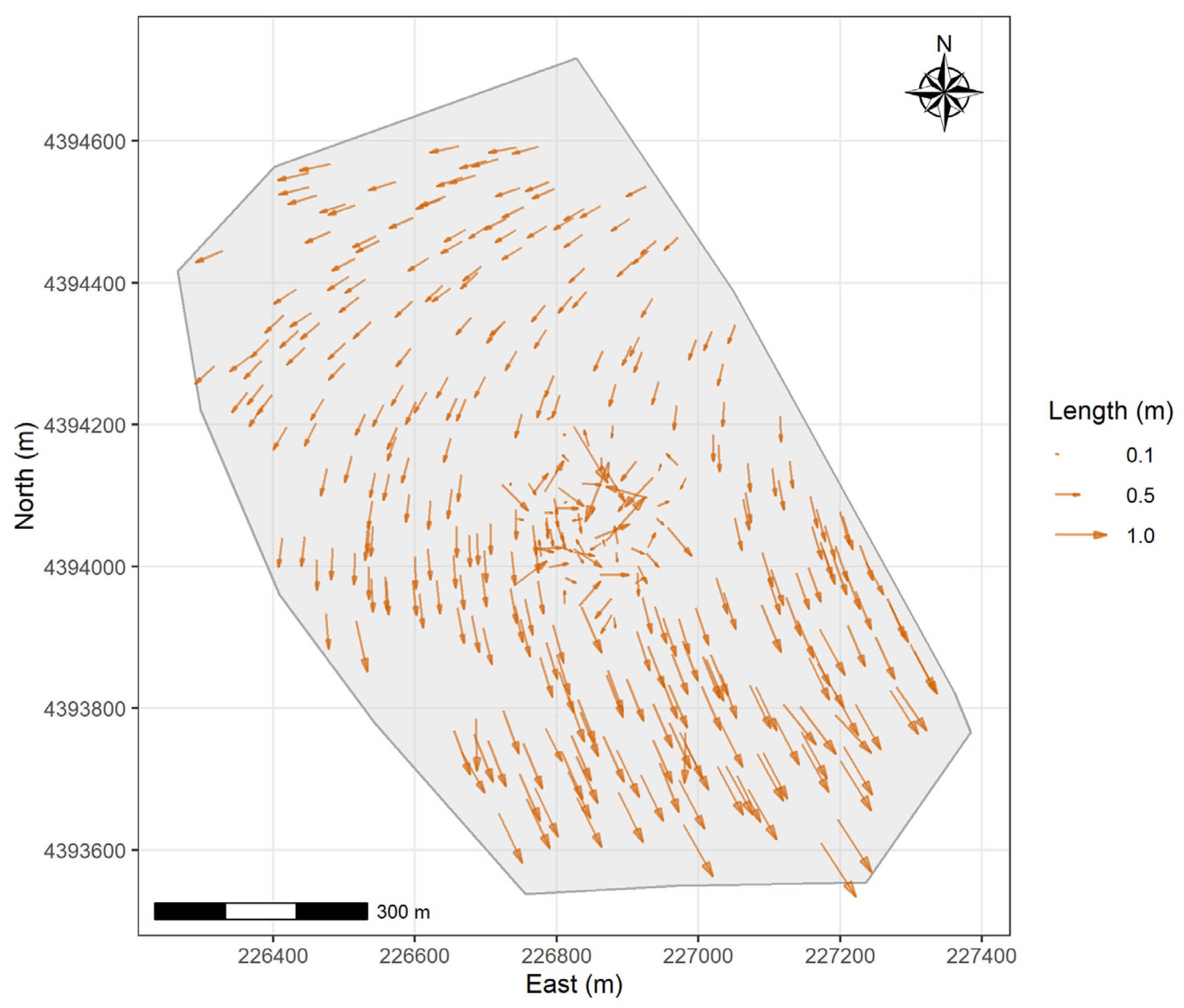
3.1.1. Stavraki

To characterize the discrepancies between the 2025 cadastral map and the 2001 land survey, we calculated the error vectors (ΔE, ΔN) and their Euclidean distances (L) of the 500 homologous points.

Table 1. The average statistical properties of $\Delta E$ and $\Delta N$ and L values for Stavraki. SD is an abbreviation for standard deviation and CV is for coefficient of variation (the absolute value of ratio of the standard deviation to the mean). All values except skew, kurtosis, and CV are in meters.

Metric	Min	Mean	Median	Max	SD	Skew	Kurtosis	CV
$\Delta E$	−0.95	0.03	0.05	1.21	0.33	−0.06	−0.65	10.67
$\Delta N$	−1.13	−0.50	−0.53	0.84	0.33	0.75	0.76	0.66
L	0.04	0.63	0.59	1.33	0.25	0.28	−0.47	0.39

presents descriptive statistics about the distribution of these error values. Prior to the application of data filtering, the root mean squared error (RMSE) on the plane of the study area was $RMS{E}_{E,N}=0.68$ m, a value that surpasses the current GNC’s geometric accuracy criterion of $RMS{E}_{(E,N)}\le 0.56$ [72].

The key observations about these values are as follows:

• Mean Error: The mean $\Delta E$ is close to zero (0.03 m), while the mean Δ$N$ is considerably larger and negative (−0.50 m). This indicates a systematic shift in the Northing direction between the 2025 and 2001 data;
• Symmetry: The near-zero skewness values for both $\Delta E$ and Δ$N$ suggest that the error distributions are approximately symmetric, although Δ$N$ has a slight positive skew;
• Tails: The negative kurtosis for ΔE indicates a platykurtic distribution that has lighter tails and a flatter peak compared to a normal distribution, whereas the positive value for ΔN is a leptokurtic distribution with heavier tails and a sharper peak;
• Variability: The CV for $\Delta E$ (10.67) is substantially larger than that for ΔNorth (0.66), indicating a greater relative variability in the Easting errors compared to the Northing errors;
• Skewness: Near-zero values suggest approximately symmetric distributions;
• Kurtosis: Low values indicate light tails, consistent with normal-like distributions.

Figure 4 depicts the spatial distribution of (ΔE, ΔN). The length of each vector represents the magnitude of the error, and its direction indicates the orientation of the discrepancy. This vector plot reveals that the errors are not randomly distributed across the study area but instead have a clear spatial structure. While a small area in the central portion of the study area shows random-error orientations and magnitudes, the dominant pattern across the rest of the region is a ring-like, counter-clockwise rotation. This pattern suggests a systematic transformation error, introduced during the integration of the Implementation Act map to the 2005 cadastral framework and indicates that the number of clusters might be two or three.

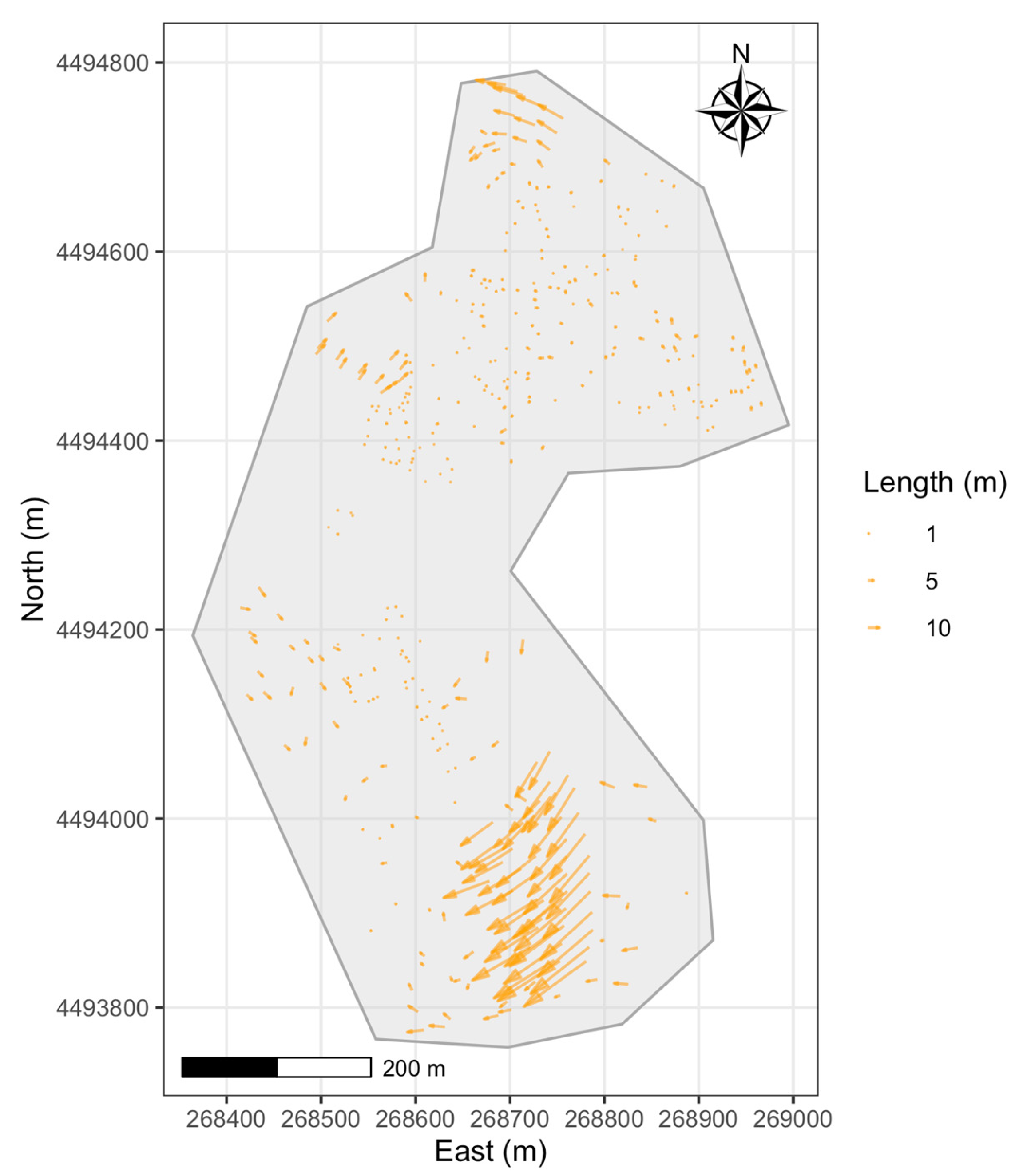
3.1.2. Kefalari

A similar exploratory analysis was conducted for the 400 homologous points in the Kefalari study area. Descriptive statistics for the error components (ΔE, ΔN, and L) are presented in

Table 2. The average statistical properties of $\Delta E$ and $\Delta N$ and L values for Kefalari. All values except skew, kurtosis, and CV are in meters.

Metric	Min	Mean	Median	Max	SD	Skew	Kurtosis	CV
$\Delta E$	−52.61	−5.26	−0.88	10.07	12.27	−2.22	4.20	2.33
$\Delta N$	−40.49	−3.27	−0.15	11.77	10.55	−2.23	4.08	3.23
L	0.18	8.82	2.44	65.14	14.91	2.30	4.12	1.69

. The $RMS{E}_{E,N}=17.22$ m, which dramatically surpasses the GNC’s geometric accuracy criterion of $RMS{E}_{(E,N)}\le 0.56$, reveals considerable positional inconsistencies.

Key observations from the Kefalari data (Table 2) include the following:

• Mean Error: Both mean ΔE and mean ΔN are considerably negative. This indicates a large, systematic shift primarily towards the west and south across the study area. The mean error magnitude is very high at 8.82 m.
• Variability: The standard deviations for both ΔE and ΔN are extremely large, signifying considerable variability and spread in the error magnitudes. The maximum error length reaches over 65 m.
• Distribution Shape (Skewness and Kurtosis): The large negative skewness values indicate that the error distributions are heavily skewed towards large negative errors. The high positive kurtosis values suggest leptokurtic distributions with heavy tails and sharp peaks, influenced by the presence of the very large error values.

Figure 5 depicts the spatial distribution of (ΔE,ΔN) for Kefalari. The vector plot clearly shows that the errors are not randomly distributed but have spatial dependency. A striking pattern emerges where the southern and the northern portion of the study display very large error vectors, predominantly oriented towards the southwest in the south and towards the northwest in the north. Also, a smaller pattern exists in the west, with large errors.

In contrast, the central parts of the study area show significantly smaller error vectors, ~1 m. This localized concentration of large errors in the southern and the northern zones suggests a spatially specific issue, possibly serious mistakes in digitizing the Land Distribution Act maps that happened during the GNC compilation process. While necessary for historical maps, rubber-sheeting itself can introduce non-linear distortions, but it is highly unlikely to be the cause of the ~60 m errors observed in the study area. The spatial form of errors indicates that the number of clusters might be between two and four.

3.2. Optimal Number of Clusters

3.2.1. Stavraki

The optimal number of clusters for each algorithm was determined as follows:

• FCM: The elbow method was used, examining visually the WSS value as a function of the number of clusters (Figure 6). A distinct ‘elbow’ is observed between two and four clusters. By the principle of parsimony (preferring simpler models), k = 3 was selected as the optimal number of clusters, as it represents the point after which the improvement in explaining the variance becomes less considerable.
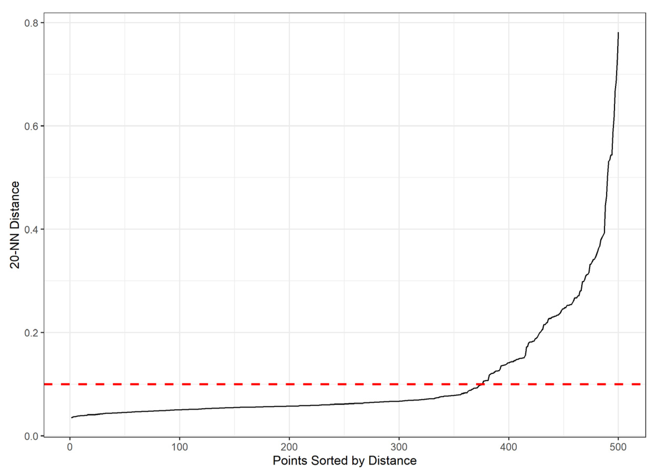
• DBSCAN: The 20-nearest neighbor distance plot (Figure 7) was examined. A visible ‘knee’ is observed around a distance of 0.10. Therefore, an ε value of 0.10 was selected. The value of $k$ was set to 20 points, to provide a stable local density estimate, which was validated through a visual inspection of the clustering results using different values of that parameter.
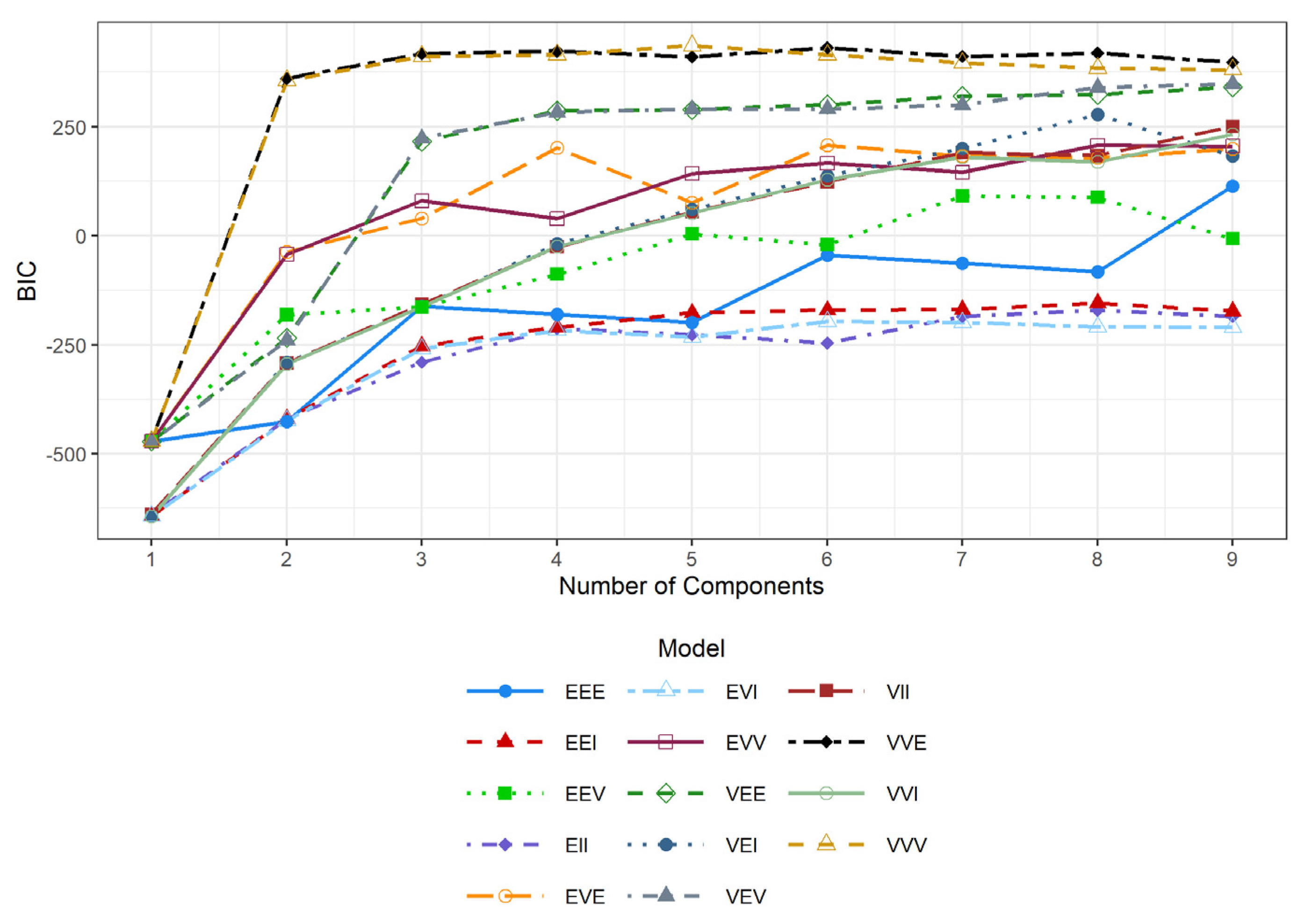
• GMM: The optimal number of components and covariance structures were selected using the Bayesian Information Criterion (BIC), which balances model fit against complexity [65] (Figure 8). Higher BIC values indicate a preferable model. Examining the BIC values across different models and component numbers, the optimal BIC was achieved for the ‘VVE’ (ellipsoidal, varying volume and shape, equal orientation) parameterization of the covariance matrix ${\Sigma }_{\kappa }$, with G = 2 components. Although models with G > 3 achieved higher BIC values, the visual inspection indicated that these led to spatially fragmented clusters lacking a clear interpretation consistent with the exploratory analysis. Therefore, the chosen model representing the peak BIC among simpler, interpretable clustering results was selected.

3.2.2. Kefalari

The optimal number of clusters for each algorithm was determined as follows:

• FCM: A very distinct ‘elbow’, compared to Stavraki dataset, is observed at k = 2, after which the decrease in WSS becomes substantially less noticeable (Figure 9).
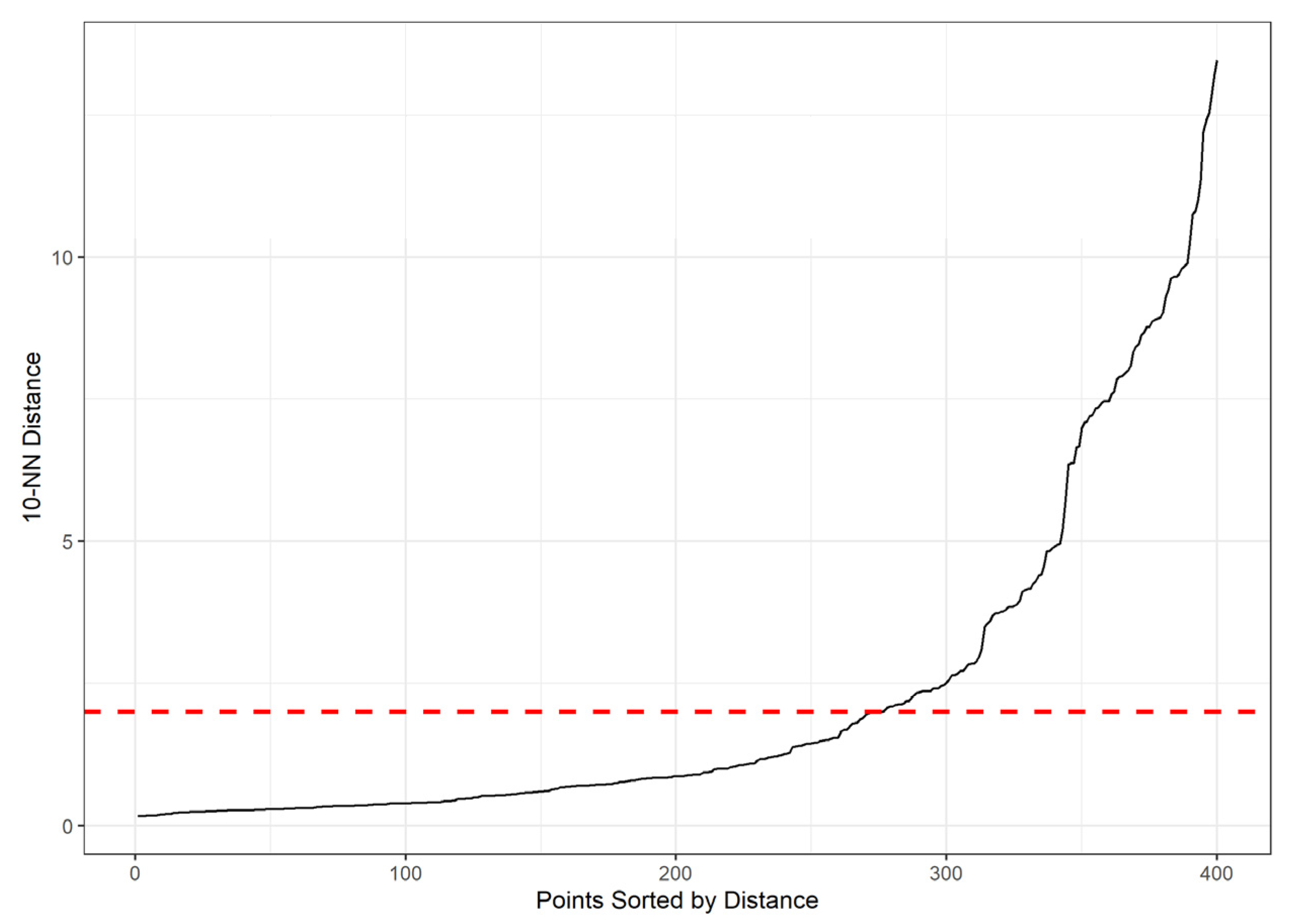
• DBSCAN: The 10-nearest neighbor distance plot (Figure 10) was examined. A visible ‘knee’, where the sorted distances begin to rise sharply, is observed around 2.0. Therefore, an ε value of 2.0 was selected.
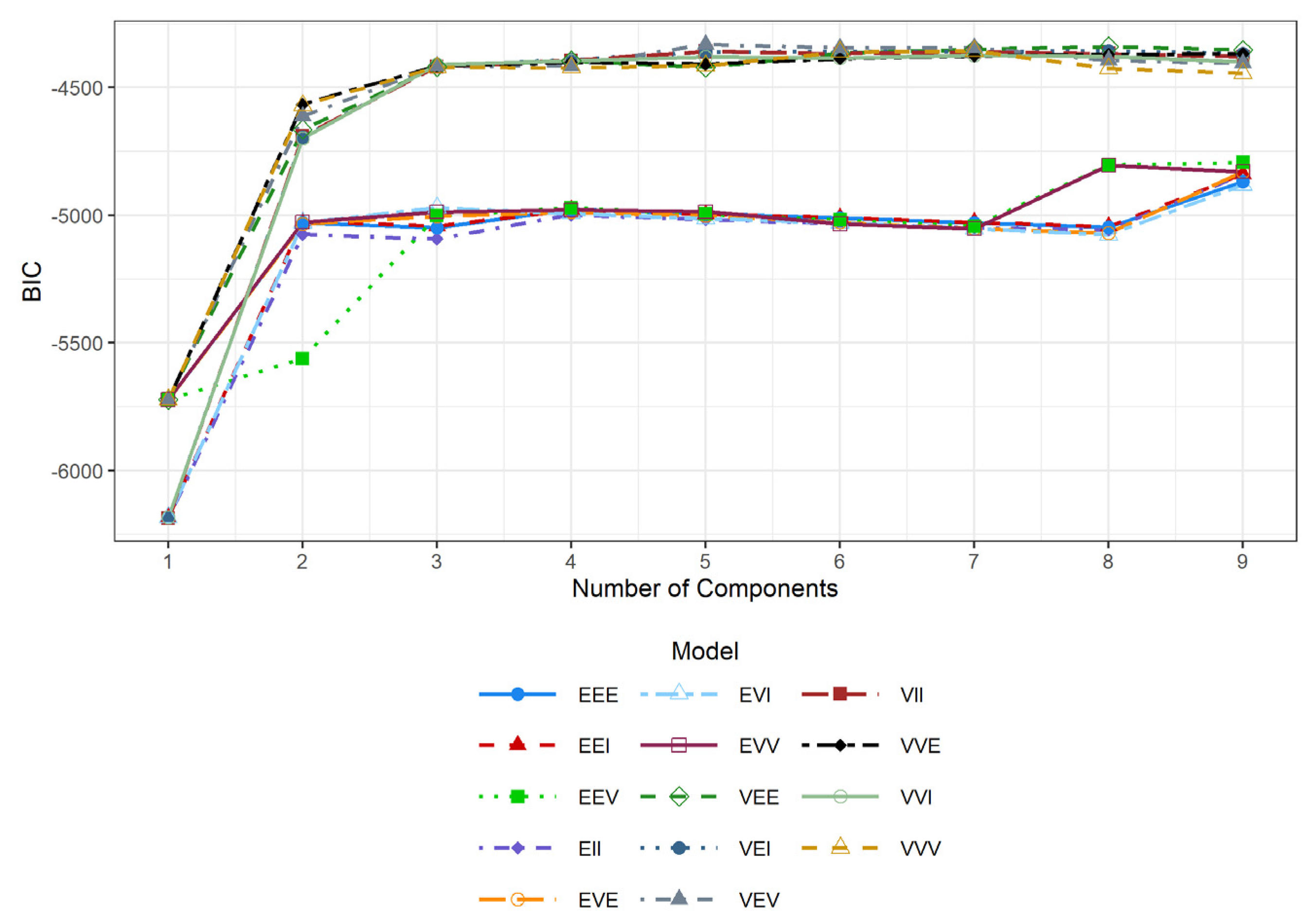
• GMM: Examining the BIC values across different models and component numbers, the optimal BIC was achieved for the ‘VVI’ (diagonal, varying volume, and shape) parameterization of the covariance matrix with G = 3 components (Figure 11). Although several models achieved higher BIC values for G > 5, these results were not consistent with the exploratory analysis.

3.3. Clustering Results—Visualizations

3.3.1. Stavraki

Figure 12, Figure 13 and Figure 14 depict the clustering results for each algorithm for Stavraki. The left panels show the error vector plot ΔE versus ΔN (i.e., in the error space), and the right ones depict the spatial distribution plot (i.e., in the actual space).

Regarding the error vector plots for each clustering algorithm, the following characteristics were observed:

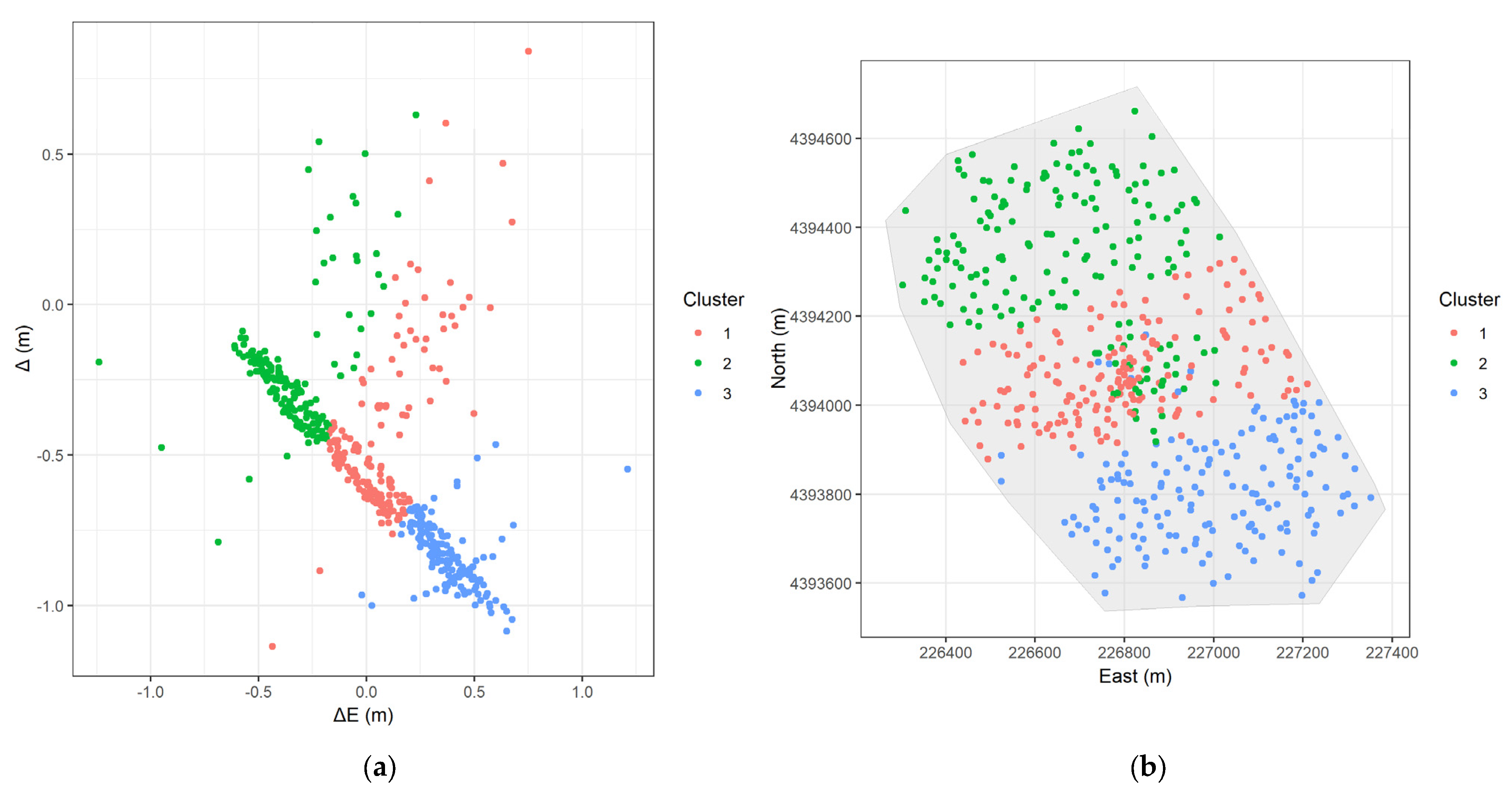
• FCM (Figure 12a): Three relatively well-separated clusters are formed. However, they do not capture the obvious linear pattern in the error space.
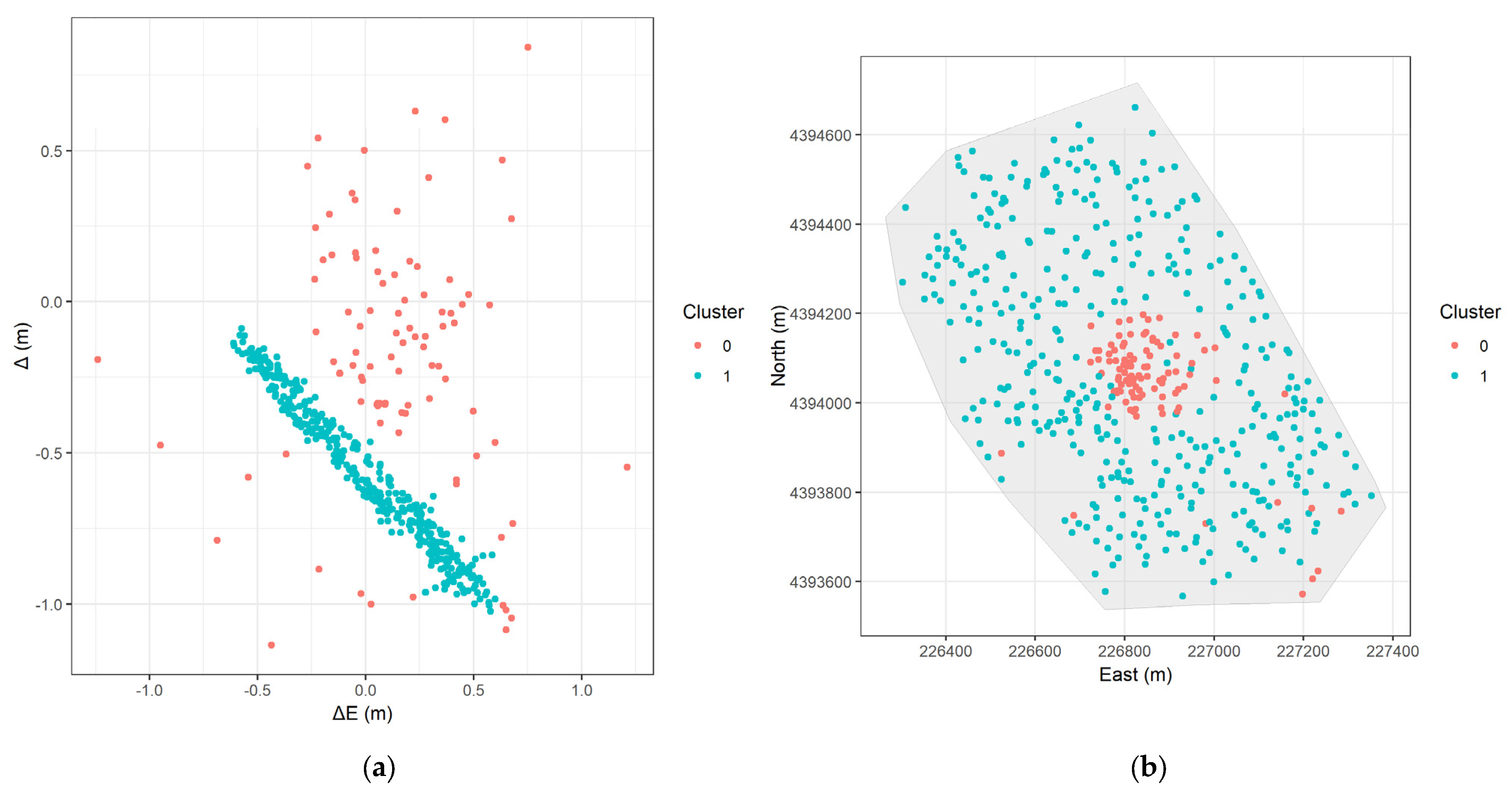
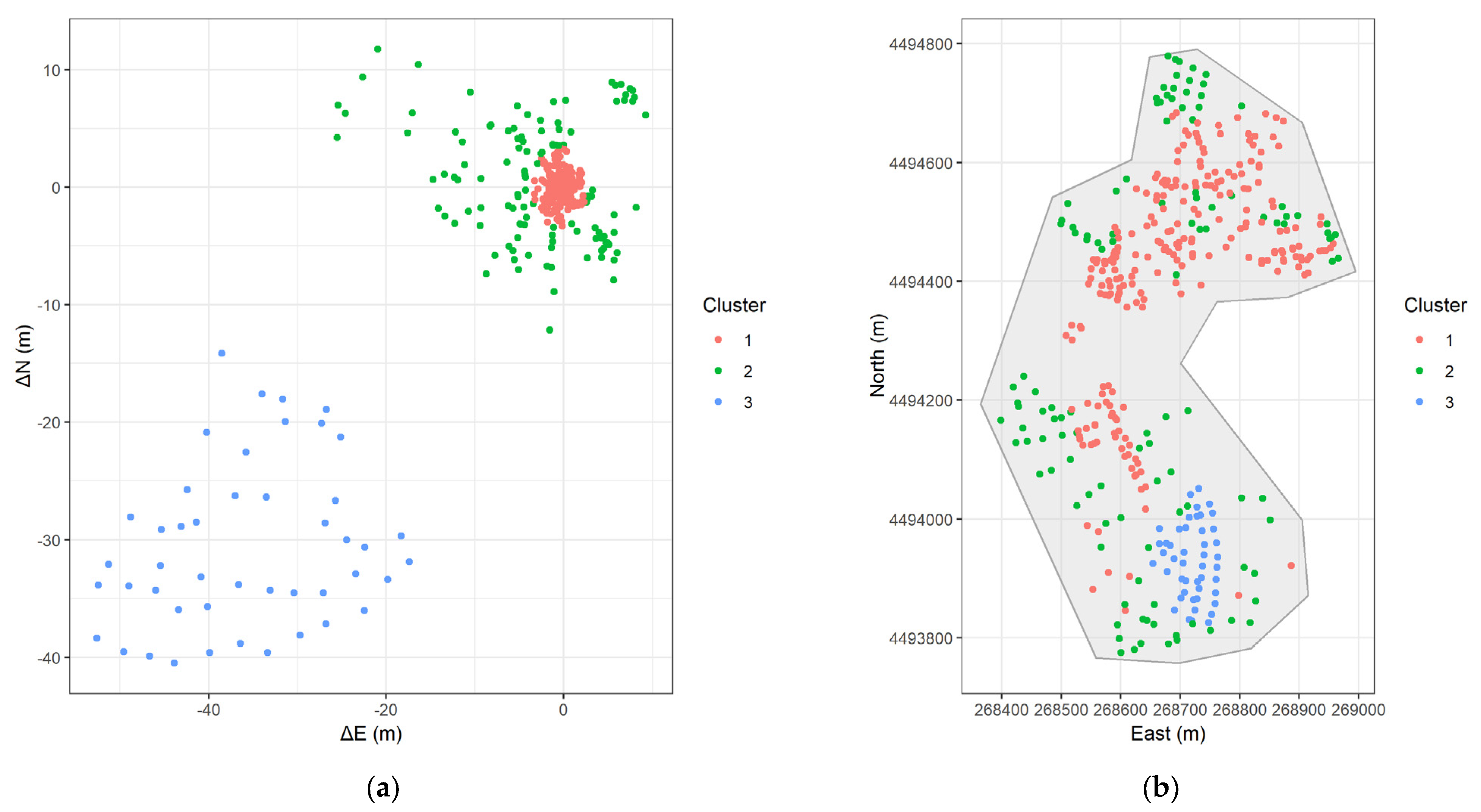
• DBSCAN (Figure 13a): The clear linear cluster (blue points) is identified as well as many noise points (red points). The linear cluster matches the suspected systematic error.
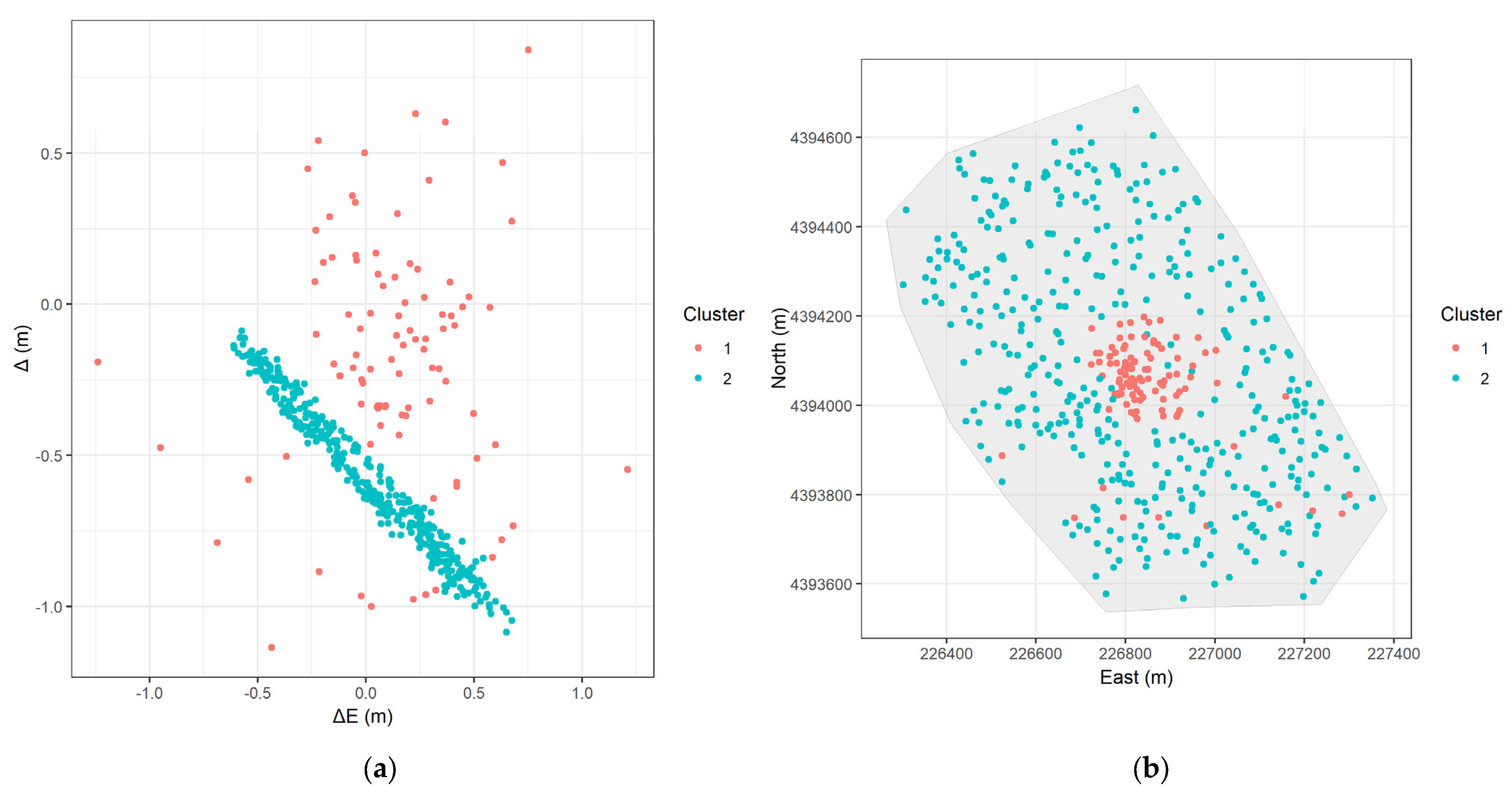
• GMM (Figure 14a): Like DBSCAN, identifies the linear cluster (blue points). However, it assigns all the other points to a separate cluster, so there are no assigned noise points.

Regarding the spatial distribution plots for each clustering algorithm, the following characteristics were observed:

• FCM (Figure 12b): The spatial distribution reveals that the clusters are not strictly distinct. The red, blue, and green points are mixed in the center of the study area and form three bands parallel to the x-axis.
• DBSCAN (Figure 13b): The blue points (the linear cluster) form a distinct, spatially contiguous region covering most of the study area, matching the area where we observed the ring-like, counter-clockwise rotational error pattern in Figure 3. The red noise points are concentrated in the central area.
• GMM (Figure 14b): The spatial distribution is very similar to DBSCAN, with the blue points forming a contiguous region corresponding to the rotational error. Most of the ‘noise’ points from DBSCAN now form the red cluster, making the distinction of signal to noise less clear.

3.3.2. Kefalari

Figure 15, Figure 16 and Figure 17 illustrate the clustering results obtained from FCM, DBSCAN, and GMM algorithms, respectively, for the Kefalari study area.

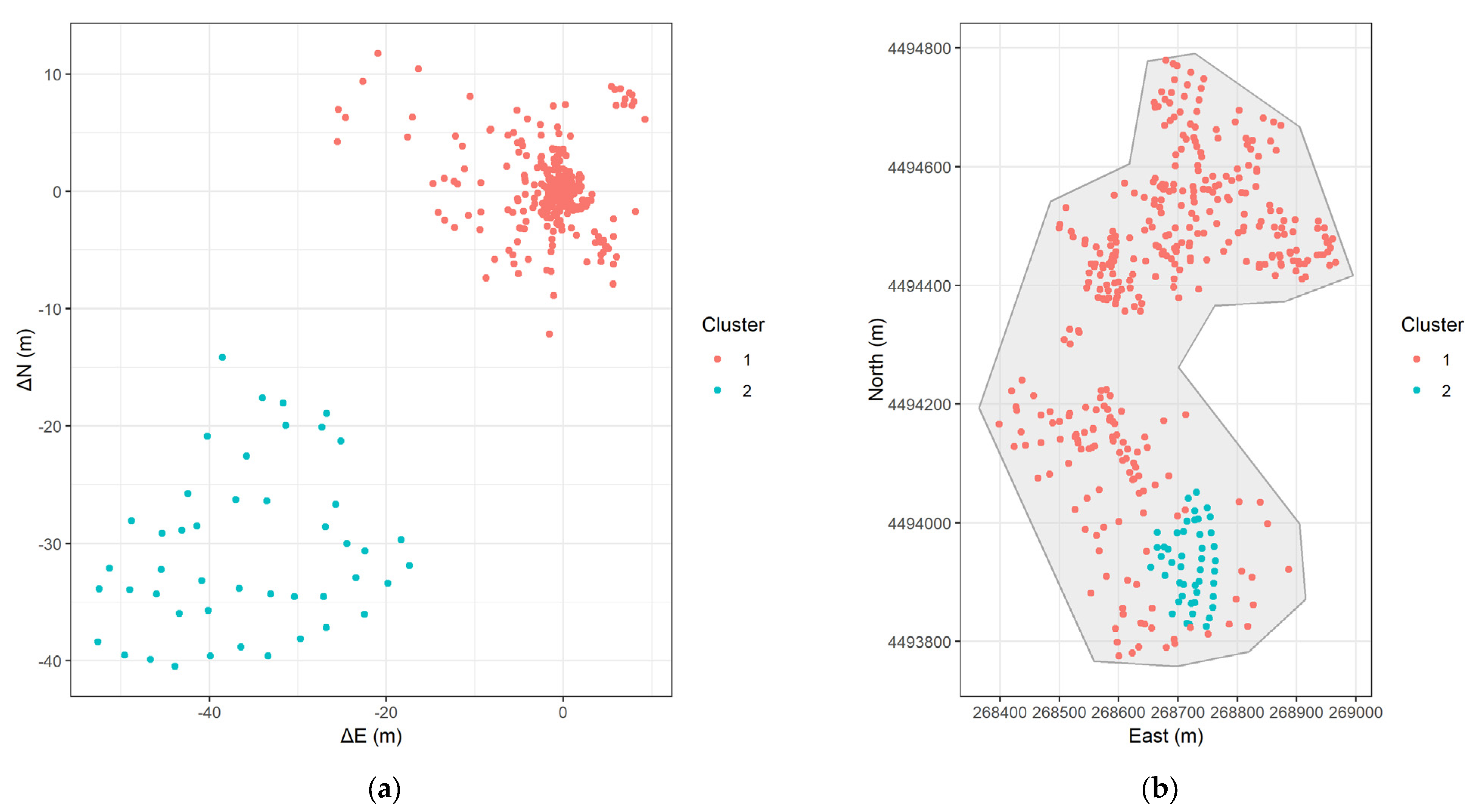
• FCM (Figure 15): Two relatively well-separated clusters are formed both in the error and the actual space. Cluster 2 (blue) exhibits large negative values, and these points are the ones already identified in the southern region of the study area.
• DBSCAN (Figure 16): The data form three clusters and a set of noise points. The noise points are characterized by very large error magnitudes in the error space. The main dense cluster (cluster 1, green) is located near the origin in the error space and corresponds to points widespread across the central study area. Two smaller distinct clusters were also identified: cluster 2 (blue) and 3 (purple), located in the mid-western area spatially.
• GMM (Figure 17): Cluster 3 (blue) is exactly the same as cluster 2 from FCM. The GMM further divided the points with smaller errors into two groups: cluster 1 (red), representing a tight core with the smallest error magnitudes near the origin in the error space and located centrally in the study area spatially (like cluster 1 of DBSCAN); and cluster 2 (green), which approximately surrounds cluster 1 both in the error and the actual space.

3.4. Silhouette Scores

3.4.1. Stavraki

The mean silhouette scores for each algorithm for Stavraki are presented in

Table 3. Mean silhouette scores (unitless) for each clustering algorithm for Stavraki.

Algorithm	Mean Silhouette Score
FCM	0.43
DBSCAN	0.32
GMM	0.25

, with FCM achieving the highest score, followed by DBSCAN and GMM. However, interpreting these scores in the context of the cadastral error patterns of the study area requires caution. The silhouette score inherently favors compact, spherical clusters, making it less suitable for evaluating clustering methods that capture more complex, non-spherical structures. DBSCAN and GMM, which captured the non-spherical linear pattern, have lower silhouette scores but provide meaningful results.

3.4.2. Kefalari

In the Kefalari study area (

Table 4. Mean silhouette scores (unitless) for each clustering algorithm for Stavraki.

Algorithm	Mean Silhouette Score
FCM	0.85
DBSCAN	0.58
GMM	0.44

), FCM, again, achieved the highest mean silhouette score, followed by DBSCAN and GMM. Recalling the silhouette score’s inherent preference for compact, spherical clusters, these results should also be interpreted with caution. Thus, despite the lowest metric scores, the GMM offers more meaningful insights into the specific error structures identified in the second study area.

3.5. Cluster Characteristics

3.5.1. Stavraki

Table 5. The average statistical properties of clusters for Stavraki. SD is an abbreviation for standard deviation.

Algorithm	Cluster	Number of Points	Mean ΔE (m)	Mean ΔN (m)	SD ΔE (m)	SD ΔN (m)	Mean Length (m)
FCM	1	178	−0.336	−0.224	0.184	0.215	0.471
	2	158	0.385	−0.831	0.139	0.11	0.923
	3	164	0.068	−0.462	0.169	0.262	0.537
DBSCAN	0 (noise)	102	0.088	−0.172	0.366	0.387	0.47
	1	398	0.008	−0.576	0.332	0.246	0.678
GMM	1	103	0.077	−0.166	0.352	0.37	0.458
	2	397	0.01	−0.579	0.336	0.249	0.682

summarizes the key statistics of the clusters identified by the three algorithms in Stavraki, including the number of points, mean displacement in the east and north directions, standard deviations, and mean error vector length. These statistics provide insights into the spatial patterns and magnitudes of cadastral errors captured by each algorithm.

Integrating the visual evidence from the spatial distribution plots with the quantitative cluster characteristics, DBSCAN effectively captures the systematic error pattern in cluster 1, with a mean ΔN of −0.57 m, confirming a consistent southward shift. Meanwhile, noise points display a smaller mean error but higher standard deviation, indicating greater variability. The GMM achieves similar results but forces all points into clusters, making the distinction between the systematic error and noise less clear. FCM, while producing well-separated clusters in the error space, fails to capture the spatial structure of the errors, demonstrating its unsuitability for this area.

The systematic error identified by both DBSCAN and GMM is characterized by a counter-clockwise rotation and a significant southward shift in a ring-shaped area. This strongly confirms the suspected issue during the integration of the Implementation Act’s outputs into the geodatabase of the GNC, where a transformation (likely involving a rotation and translation) was incorrectly applied to a ring-shaped portion of the study area. The points identified as noise by DBSCAN and as the cluster number one by the GMM represent the central area that has more complex, non-systematic errors.

3.5.2. Kefalari

Key statistics for the clusters identified by the three algorithms in Kefalari are also summarized in

Table 6. The average statistical properties of clusters for Kefalari. SD is an abbreviation for standard deviation.

Algorithm	Cluster	Number of Points	Mean ΔE (m)	Mean ΔN (m)	SD ΔE (m)	SD ΔN (m)	Mean Length (m)
FCM	1	354	−1.35	0.215	4.66	3.12	3.74
	2	46	−35.6	−30.6	9.83	6.93	47.5
DBSCAN	0 (noise)	76	−26.4	−17.8	14.6	17.2	34.5
	1	296	−0.91	0.06	1.83	2.09	2.23
	2	17	4.67	−4.88	0.918	1.28	6.83
	3	11	7.08	7.88	1.11	0.827	10.7
GMM	1	237	−0.43	0.037	1.08	1.18	1.44
	2	117	−3.21	0.575	7.64	5.16	8.4
	3	46	−35.6	−30.6	9.83	6.93	47.5

.

Combining the visual evidence (Figure 5, Figure 15, Figure 16 and Figure 17) with the quantitative characteristics (Table 6), distinct error behaviors exist in Kefalari. Both FCM (Cluster 2) and the GMM (Cluster 3) cleanly identify the group of 46 points at the south with the very large systematic displacement. DBSCAN identifies a larger set of 76 points as noise, encompassing the two different areas with the biggest errors values. For the points with smaller errors, concentrated in the central area, the GMM provides the finest separation: cluster 1 shows a minimal error (mean length 1.44 m, SDs~1 m), while cluster 2 captures surrounding points with slightly larger, more variable errors (mean length 8.4 m, SDs~5–8 m). DBSCAN similarly identifies these small errors in a cluster (mean length 2.23 m, SDs~2 m), isolating two additional small, tight clusters (2 and 3, indicating an erroneous translation). FCM groups most points with relatively smaller errors into a single, more scattered cluster (cluster 1, mean length 3.74 m, SDs~3–5 m).

The analysis reveals two primary error phenomena in Kefalari. Firstly, a significant systematic error, characterized by a large southwesterly shift (~47.5 m), affects a distinct subset of points located predominantly in the southern part of the study area. This represents a significant processing mistake specific to this sub-area, in which blocks of parcels are misplaced. Secondly, most points, primarily in the northern and central regions, exhibit much smaller errors. DBSCAN identified the large, problematic errors as noise/outliers, while the GMM excels in partitioning both the large systematic error group and the different levels of smaller errors that represent different areas. FCM provides a clear, albeit less detailed, separation between the two main error types.

4. Discussion

This study successfully demonstrates the utility of unsupervised machine learning algorithms for efficiently identifying and characterizing systematic spatial errors within cadastral data across two case studies in Greece with different error sources: (a) Stavraki was affected by modern survey integration issues and (b) Kefalari was impacted by historical diagram integration challenges and gross errors. The findings underscore the method’s applicability in diverse cadastral contexts facing various positional accuracy problems.

The application of clustering algorithms revealed the presence of different error characteristics in the two study areas, underscoring the heterogeneity of issues within the GNC and the adaptability of the proposed approach:

• In the first study area, the analysis uncovered a dominant, systematic counter-clockwise rotational error pattern affecting a large, ring-shaped portion of the area, surrounding a central zone with smaller, more random errors. This pattern strongly suggests that a transformation error was introduced during the integration of the precise 2001 Implementing Act data into the GNC geodatabase in 2005, as suspected by local surveyors. Both DBSCAN and the GMM effectively captured this structure. DBSCAN excelled by explicitly isolating the central, less systematic errors as ‘noise,’ providing a clear distinction between the main systematic issue and other variations. In the contrary, FCM failed to capture these error patterns.
• In the second study area, the errors were characterized by significant magnitudes and strong spatial localization. The analysis confirmed the presence of the distinct sub-area in the south with a very large displacement, contrasting with other areas with relatively smaller errors. This points to gross errors that occurred during the georeferencing and digitization of the historical 1978 Land Distribution diagram into the GCN, affecting specific parts of the study area differently. In this area, the GMM excelled, providing the finest result, partitioning the data into three meaningful clusters: the large systematic error zone, a central area with minimal errors, and an intermediate surrounding zone. DBSCAN identified the largest errors as noise; however, possibly due to significant differences in data densities, it did not perform as well as the GMM. FCM provided a coarser, though somewhat useful, separation in the actual and error space between the very large displacement area and the rest.

The interpretation of these errors relies not solely on summary statistics but on a combination of visual analysis and the spatial patterns revealed by the clustering algorithms. This finding depicts the challenges that may arise in order to improve the positional accuracy in LASs, particularly when data are coming from various sources and historical maps [73,74,75]. It also highlights the need for cadastral data renewal, to address errors and inconsistencies, as reported in the literature.

The comparison of the algorithms across different areas emphasizes the importance of choosing one appropriate to the specific domain’s data structure, in our case real-world cadastral data. DBSCAN’s noise handling is advantageous when a primary systematic pattern needs separation from random variations (Stavraki). The GMM’s probabilistic framework and flexibility in cluster shapes proved more effective in modeling multiple error distributions, including localized gross errors alongside smaller ones (Kefalari).

Furthermore, this study highlights an inherent challenge in unsupervised clustering, and determining the optimal number of clusters (k for FCM, G for GMM) or appropriate parameters (ε and minPts for DBSCAN) requires careful consideration. While methods like the elbow plot, kNN distance plot, and BIC provide valuable guidance, they are heuristics. As demonstrated, with the BIC potentially suggesting overly complex models, statistical criteria must be validated by visual inspection and spatial interpretability of the clustering results. The ‘optimal’ parameters were ultimately those that produced spatially consistent and meaningful clusters, corresponding to visually distinguishable patterns in both the error and the actual geometric space. This underscores the necessity of combining quantitative guidance with qualitative, domain-specific assessments.

Moreover, the popular silhouette score proved potentially misleading. While FCM achieved systematically higher scores in both cases, its results were less interpretable spatially compared to DBSCAN and the GMM, especially in the first study area, reinforcing the limitations of relying exclusively on metrics that favor compact, convex clusters, especially when dealing with complex, spatial error patterns.

The findings of this study have a direct application to the GNC and similar LASs facing accuracy issues. For example, the identified region with the systematic error in the first study area provides a clear target for corrections. Instead of conducting a re-survey of the entire area, resources can be directed to this region, using a simple transformation of the parcels, such as the Helmert transformation [76], to address the issue. On the other hand, the identification of specific zones with gross errors in the second study area calls for immediate action, as well as the focused investigation and subsequent correction of the problem. This approach has the potential to reduce the cost and time required for cadastral map accuracy improvement in Greece.

Additionally, our results support the principles of FFPLA [14]. Clustering can be used as a ‘minimum viable’ method to identify and prioritize areas for improvement, supporting the FFPLA concept of upgradability. The identified clusters represent areas where the cadastral data in both study areas are not currently ‘fit-for-purpose’ in terms of positional accuracy, and the clustering results provide a roadmap for targeted and economical corrections.

To our knowledge, this is the first study applying and comparing multiple unsupervised clustering techniques specifically for the detection and characterization of systematic spatial error patterns in cadastral vector data. By interpreting the clusters in relation to known cadastral processes and error sources, the study moves beyond simple pattern detection to provide actionable insights for data quality improvement. This automated ability represents a valuable step towards more efficient LAS maintenance and supports the GNC’s stated commitment to use advanced technologies like AI. The identified clusters could serve as spatially explicit inputs for subsequent supervised learning models aimed at automated geometric correction, an area where AI applications in LASs remain scarce.

5. Conclusions

This study successfully demonstrates that unsupervised algorithms can effectively identify and characterize different types of spatial errors within digital cadastral maps. The practical value of this approach lies in its potential to automate the diagnosis of problematic regions regarding spatial accuracy within cadastral datasets. This enables targeted, cost-effective correction efforts, directly supporting the goals of cadastral data renewal for systems like the Greek National Cadastre and aligning with the incremental improvement philosophy of fit-for-purpose land administration.

This research has limitations because the analysis focuses on two study areas from the Greek National Cadastre. However, the methodology itself as presented is transferable to other land administration systems contexts, even if the error patterns differ, as exemplified by the two study areas’ different error spatial characteristics and origins. In addition, while clustering identifies the presence and location of systematic errors, it does not, by itself, provide the solution to correct them. Therefore, further work is needed towards the development of automated improvement methods.

Future research should focus on validating this methodology across more diverse cadastral areas and error types, potentially integrating expert knowledge or exploring other clustering and machine learning approaches. Integrating expert knowledge through semi-supervised or active learning could improve results. Future work should focus on developing automated correction methods based on these findings, leading to a streamlined workflow for cadastral map improvement, with a goal for more reliable, fit-for-purpose land administration systems.

References

- Movahhed Moghaddam, S.; Azadi, H.; Sklenička, P.; Janečková, K. Impacts of Land Tenure Security on the Conversion of Agricultural Land to Urban Use. Land Degrad. Dev. 2025. [Google Scholar] [CrossRef]
- Bydłosz, J. The Application of the Land Administration Domain Model in Building a Country Profile for the Polish Cadastre. Land Use Policy 2015, 49, 598–605. [Google Scholar] [CrossRef]
- Uşak, B.; Çağdaş, V.; Kara, A. Current Cadastral Trends—A Literature Review of the Last Decade. Land 2024, 13, 2100. [Google Scholar] [CrossRef]
- Aguzarova, L.A.; Aguzarova, F.S. On the Issue of Cadastral Value and Its Impact on Property Taxation in the Russian Federation. In Business 4.0 as a Subject of the Digital Economy; Popkova, E.G., Ed.; Advances in Science, Technology & Innovation; Springer International Publishing: Cham, Switzerland, 2022; pp. 595–599. ISBN 978-3-030-90323-7. [Google Scholar]
- El Ayachi, M.; Semlali, E.H. Digital Cadastral Map, a Multipurpose Tool for Sustainable Development. In Proceedings of the International Conference on Spatial Information for Sustainable Development, Nairobi, Kenya, 2–5 October 2001; pp. 2–5. [Google Scholar]
- Jahani Chehrehbargh, F.; Rajabifard, A.; Atazadeh, B.; Steudler, D. Current Challenges and Strategic Directions for Land Administration System Modernisation in Indonesia. J. Spat. Sci. 2024, 69, 1097–1129. [Google Scholar] [CrossRef]
- Hashim, N.M.; Omar, A.H.; Ramli, S.N.M.; Omar, K.M.; Din, N. Cadastral Database Positional Accuracy Improvement. Int. Arch. Photogramm. Remote Sens. Spat. Inf. Sci. 2017, 42, 91–96. [Google Scholar] [CrossRef]
- Ercan, O. Evolution of the Cadastre Renewal Understanding in Türkiye: A Fit-for-Purpose Renewal Model Proposal. Land Use Policy 2023, 131, 106755. [Google Scholar] [CrossRef]
- Kysel’, P.; Hudecová, L. Testing of a New Way of Cadastral Maps Renewal in Slovakia. Géod. Vestn. 2022, 66, 521–535. [Google Scholar]
- Lauhkonen, H. Cadastral Renewal in Finland-The Challenges of Implementing LIS. GIM Int. 2007, 21, 42. [Google Scholar]
- Cetl, V.; Roic, M.; Ivic, S.M. Towards a Real Property Cadastre in Croatia. Surv. Rev. 2012, 44, 17–22. [Google Scholar] [CrossRef]
- Roić, M.; Križanović, J.; Pivac, D. An Approach to Resolve Inconsistencies of Data in the Cadastre. Land 2021, 10, 70. [Google Scholar] [CrossRef]
- Thompson, R.J. A Model for the Creation and Progressive Improvement of a Digital Cadastral Data Base. Land Use Policy 2015, 49, 565–576. [Google Scholar] [CrossRef]
- Bennett, R.M.; Unger, E.-M.; Lemmen, C.; Dijkstra, P. Land Administration Maintenance: A Review of the Persistent Problem and Emerging Fit-for-Purpose Solutions. Land 2021, 10, 509. [Google Scholar] [CrossRef]
- Morgenstern, D.; Prell, K.M.; Riemer, H.G. Digitisation and Geometrical Improvement of Inhomogeneous Cadastral Maps. Surv. Rev. 1989, 30, 149–159. [Google Scholar] [CrossRef]
- Tamim, N.S. A Methodology to Create a Digital Cadastral Overlay Through Upgrading Digitized Cadastral Data; The Ohio State University: Columbus, OH, USA, 1992. [Google Scholar]
- Tuno, N.; Mulahusić, A.; Kogoj, D. Improving the Positional Accuracy of Digital Cadastral Maps through Optimal Geometric Transformation. J. Surv. Eng. 2017, 143, 05017002. [Google Scholar] [CrossRef]
- Čeh, M.; Gielsdorf, F.; Trobec, B.; Krivic, M.; Lisec, A. Improving the Positional Accuracy of Traditional Cadastral Index Maps with Membrane Adjustment in Slovenia. ISPRS Int. J. Geo-Inf. 2019, 8, 338. [Google Scholar] [CrossRef]
- Franken, J.; Florijn, W.; Hoekstra, M.; Hagemans, E. Rebuilding the Cadastral Map of The Netherlands, the Artificial Intelligence Solution. In Proceedings of the FIG Working Week, Amsterdam, The Netherlands, 10–14 May 2020. [Google Scholar]
- Petitpierre, R.; Guhennec, P. Effective Annotation for the Automatic Vectorization of Cadastral Maps. Digit. Scholarsh. Humanit. 2023, 38, 1227–1237. [Google Scholar] [CrossRef]
- Hastie, T.; Friedman, J.; Tibshirani, R. The Elements of Statistical Learning, 2nd ed.; Springer Series in Statistics; Springer: New York, NY, USA, 2001; ISBN 978-1-4899-0519-2. [Google Scholar]
- Tyagi, A.K.; Chahal, P. Artificial Intelligence and Machine Learning Algorithms. In Challenges and Applications for Implementing Machine Learning in Computer Vision; IGI Global Scientific Publishing: Hershey, PA, USA, 2020; pp. 188–219. [Google Scholar]
- Hartigan, J.A. Clustering Algorithms; John Wiley & Sons Inc.: New York, NY, USA, 1975; ISBN 978-0-471-35645-5. [Google Scholar]
- Jain, A.K.; Duin, R.P.W.; Mao, J. Statistical Pattern Recognition: A Review. IEEE Trans. Pattern Anal. Mach. Intell. 2000, 22, 4–37. [Google Scholar] [CrossRef]
- Oyewole, G.J.; Thopil, G.A. Data Clustering: Application and Trends. Artif. Intell. Rev. 2023, 56, 6439–6475. [Google Scholar] [CrossRef]
- Han, J.; Pei, J.; Tong, H. Data Mining: Concepts and Techniques; Morgan Kaufmann: Burlington, MA, USA, 2022. [Google Scholar]
- Grubesic, T.H.; Wei, R.; Murray, A.T. Spatial Clustering Overview and Comparison: Accuracy, Sensitivity, and Computational Expense. Ann. Assoc. Am. Geogr. 2014, 104, 1134–1156. [Google Scholar] [CrossRef]
- Wang, H.; Song, C.; Wang, J.; Gao, P. A Raster-Based Spatial Clustering Method with Robustness to Spatial Outliers. Sci. Rep. 2024, 14, 4103. [Google Scholar] [CrossRef]
- Xie, Y.; Shekhar, S.; Li, Y. Statistically-Robust Clustering Techniques for Mapping Spatial Hotspots: A Survey. ACM Comput. Surv. 2023, 55, 3487893. [Google Scholar] [CrossRef]
- Vantas, K.; Sidiropoulos, E.; Loukas, A. Robustness Spatiotemporal Clustering and Trend Detection of Rainfall Erosivity Density in Greece. Water 2019, 11, 1050. [Google Scholar] [CrossRef]
- Milligan, G.W.; Cooper, M.C. An Examination of Procedures for Determining the Number of Clusters in a Data Set. Psychometrika 1985, 50, 159–179. [Google Scholar] [CrossRef]
- Charrad, M.; Ghazzali, N.; Boiteau, V.; Niknafs, A. NbClust: An R Package for Determining the Relevant Number of Clusters in a Data Set. J. Stat. Softw. 2014, 61, 1–36. [Google Scholar] [CrossRef]
- Vantas, K.; Sidiropoulos, E. Intra-Storm Pattern Recognition through Fuzzy Clustering. Hydrology 2021, 8, 57. [Google Scholar] [CrossRef]
- Potsiou, C.; Volakakis, M.; Doublidis, P. Hellenic Cadastre: State of the Art Experience, Proposals and Future Strategies. Comput. Environ. Urban Syst. 2001, 25, 445–476. [Google Scholar] [CrossRef]
- Hellenic Republic. Law 2308: Cadastral Survey for the Creation of a National Cadastre. Procedure Up to the First Entries in the Cadastral Books and Other Provisions; Hellenic Republic: Athens, Greece, 1995; p. 8. [Google Scholar]
- Hellenic Republic. Law 2664: National Cadastre and Other Provisions; Hellenic Republic: Athens, Greece, 1998; p. 20. [Google Scholar]
- Arvanitis, A. Cadastre 2020; Editions Ziti: Thessaloniki, Greece, 2014; ISBN 978-960-456-423-1. [Google Scholar]
- Vantas, K. Improving the Positional Accuracy of Cadastral Maps via Machine Learning Methods; Aristotle University of Thessaloniki: Thessaloniki, Greece, 2022. [Google Scholar]
- Cadastre: The First Public Agency to Integrate Artificial Intelligence. Available online: https://www.ktimatologio.gr/grafeio-tipou/deltia-tipou/1493 (accessed on 10 March 2025). (In Greek).
- Hellenic Republic. Law 1337: Expansion of Urban Plans, Residential Development and Related Regulations; Hellenic Republic: Athens, Greece, 1983; p. 16. [Google Scholar]
- Greek National Cadastre—Open Data Portal. Available online: https://data.ktimatologio.gr/ (accessed on 11 March 2025).
- Veis, G. Reference Systems and the Realization of the Hellenic Geodetic Reference System 1987. In Technika Chronika; Technical Chamber of Greece: Athens, Greece, 1995; pp. 16–22. [Google Scholar]
- Fotiou, A.; Livieratos, E. Geometric Geodesy and Networks; Editions Ziti: Thessaloniki, Greece, 2000; ISBN 960-431-612-5. [Google Scholar]
- QGIS Geographic Information System, Version 3.42; QGIS Development Team, 2025.
- Hellenic Mapping and Cadastral Organization. Tables of Coefficients for Coordinates Transformation of the Hellenic Area; HEMCO: Athens, Greece, 1995. [Google Scholar]
- R: A Language and Environment for Statistical Computing; Version 4.4.2; Foundation for Statistical Computing: Vienna, Austria, 2025.
- Maechler, M.; Rousseeuw, P.; Struyf, A.S.; Hubert, M.; Hornik, K.; Studer, M.; Roudier, P.; Gonzalez, J.; Kozlowski, K.; Schubert, E.; et al. Cluster: “Finding Groups in Data”, Version 2.1.8. 2024.
- Hahsler, M.; Piekenbrock, M.; Arya, S.; Mount, D.; Malzer, C. Dbscan: Density-Based Spatial Clustering of Applications with Noise (DBSCAN) and Related Algorithms, Version 1.2.2. 2025.
- Mclust: Gaussian Mixture Modelling for Model-Based Clustering, Classification, and Density Estimation, Version 6.1.1. 2024.
- Fraley, C.; Raftery, A.E.; Scrucca, L.; Murphy, T.B.; Fop, M. Factoextra: Extract and Visualize the Results of Multivariate Data Analyses; Version 1.0.7; Kassambara, A., Mundt, F., Eds.; 2020. [Google Scholar]
- Wickham, H.; Chang, W.; Henry, L.; Pedersen, T.L.; Takahashi, K.; Wilke, C.; Woo, K.; Yutani, H.; Dunnington, D.; van den Brand, T.; et al. Ggplot2: Create Elegant Data Visualisations Using the Grammar of Graphics; Version 3.5.1; 2024. [Google Scholar]
- Pebesma, E.; Bivand, R.; Racine, E.; Sumner, M.; Cook, I.; Keitt, T.; Lovelace, R.; Wickham, H.; Ooms, J.; Müller, K.; et al. Sf: Simple Features for R, Version 1.0-20. 2024.
- Bishop, C.M.; Nasrabadi, N.M. Pattern Recognition and Machine Learning; Springer: Berlin/Heidelberg, Germany, 2006; Volume 4. [Google Scholar]
- Sarle, W.S. Finding Groups in Data: An Introduction to Cluster Analysis. J. Am. Stat. Assoc. 1991, 86, 830. [Google Scholar] [CrossRef]
- Dunn, J.C. A Fuzzy Relative of the ISODATA Process and Its Use in Detecting Compact Well-Separated Clusters. J. Cybern. 1973, 3, 32–57. [Google Scholar] [CrossRef]
- Bezdek, J.C. Pattern Recognition with Fuzzy Objective Function Algorithms; Springer Science & Business Media: Berlin/Heidelberg, Germany, 2013. [Google Scholar]
- Nayak, J.; Naik, B.; Behera, H.S. Fuzzy C-Means (FCM) Clustering Algorithm: A Decade Review from 2000 to 2014. In Proceedings of the Computational Intelligence in Data Mining—Volume 2, Proceedings of the International Conference on CIDM, 20–21 December 2014; Jain, L.C., Behera, H.S., Mandal, J.K., Mohapatra, D.P., Eds.; Springer: New Delhi, India, 2015; pp. 133–149. [Google Scholar]
- Huang, M.; Xia, Z.; Wang, H.; Zeng, Q.; Wang, Q. The Range of the Value for the Fuzzifier of the Fuzzy C-Means Algorithm. Pattern Recognit. Lett. 2012, 33, 2280–2284. [Google Scholar] [CrossRef]
- Bezdek, J.C. Objective Function Clustering. In Pattern Recognition with Fuzzy Objective Function Algorithms; Springer: Boston, MA, USA, 1981; pp. 43–93. ISBN 978-1-4757-0452-5. [Google Scholar]
- Syakur, M.A.; Khotimah, B.K.; Rochman, E.M.S.; Satoto, B.D. Integration K-Means Clustering Method and Elbow Method for Identification of the Best Customer Profile Cluster. In Proceedings of the IOP Conference Series: Materials Science and Engineering, Novi Sad, Serbia, 6–8 June 2018; IOP Publishing: Bristol, UK, 2018; Volume 336, p. 012017. [Google Scholar]
- Ester, M.; Kriegel, H.-P.; Sander, J.; Xu, X. Density-Based Spatial Clustering of Applications with Noise. In Proceedings of the 2nd International Conference on Knowledge Discovery and Data Mining, Portland, OR, USA, 2–4 August 1996; Volume 240. [Google Scholar]
- Kriegel, H.; Kröger, P.; Sander, J.; Zimek, A. Density-based Clustering. WIREs Data Min. Knowl. 2011, 1, 231–240. [Google Scholar] [CrossRef]
- Hahsler, M.; Piekenbrock, M.; Doran, D. Dbscan: Fast Density-Based Clustering with R. J. Stat. Softw. 2019, 91, 1–30. [Google Scholar] [CrossRef]
- Reynolds, D.A. Gaussian Mixture Models. Encycl. Biom. 2009, 741, 3. [Google Scholar]
- Scrucca, L.; Fraley, C.; Murphy, T.B.; Raftery, A.E. Model-Based Clustering, Classification, and Density Estimation Using Mclust in R; Chapman and Hall/CRC: Boca Raton, FL, USA, 2023; ISBN 978-1-032-23495-3. [Google Scholar]
- Scrucca, L.; Fop, M.; Murphy, T.B.; Raftery, A.E. Mclust 5: Clustering, Classification and Density Estimation Using Gaussian Finite Mixture Models. R J. 2016, 8, 289. [Google Scholar] [CrossRef]
- Fraley, C.; Raftery, A.E. Model-Based Clustering, Discriminant Analysis, and Density Estimation. J. Am. Stat. Assoc. 2002, 97, 611–631. [Google Scholar] [CrossRef]
- Yang, M.-S.; Lai, C.-Y.; Lin, C.-Y. A Robust EM Clustering Algorithm for Gaussian Mixture Models. Pattern Recognit. 2012, 45, 3950–3961. [Google Scholar] [CrossRef]
- Gupta, M.R.; Chen, Y. Theory and Use of the EM Algorithm. Found. Trends® Signal Process. 2011, 4, 223–296. [Google Scholar] [CrossRef]
- Shahapure, K.R.; Nicholas, C. Cluster Quality Analysis Using Silhouette Score. In Proceedings of the 2020 IEEE 7th International Conference on Data Science and Advanced Analytics (DSAA), Sydney, NSW, Australia, 6–9 October 2020; IEEE: Piscataway, NJ, USA, 2020; pp. 747–748. [Google Scholar]
- Arbelaitz, O.; Gurrutxaga, I.; Muguerza, J.; Pérez, J.M.; Perona, I. An Extensive Comparative Study of Cluster Validity Indices. Pattern Recognit. 2013, 46, 243–256. [Google Scholar] [CrossRef]
- Hellenic Republic. Approval of Technical Specifications and the Regulation of Estimated Fees for Cadastral Survey Studies for the Creation of the National Cadastre in the Remaining Areas of the Country; Ministry of Environment and Energy: Athens, Greece, 2016; p. 228.
- Sisman, Y. Coordinate Transformation of Cadastral Maps Using Different Adjustment Methods. J. Chin. Inst. Eng. 2014, 37, 869–882. [Google Scholar] [CrossRef]
- Tong, X.; Liang, D.; Xu, G.; Zhang, S. Positional Accuracy Improvement: A Comparative Study in Shanghai, China. Int. J. Geogr. Inf. Sci. 2011, 25, 1147–1171. [Google Scholar] [CrossRef]
- Manzano-Agugliaro, F.; Montoya, F.G.; San-Antonio-Gómez, C.; López-Márquez, S.; Aguilera, M.J.; Gil, C. The Assessment of Evolutionary Algorithms for Analyzing the Positional Accuracy and Uncertainty of Maps. Expert Syst. Appl. 2014, 41, 6346–6360. [Google Scholar] [CrossRef]
- Watson, G.A. Computing Helmert Transformations. J. Comput. Appl. Math. 2006, 197, 387–394. [Google Scholar] [CrossRef]