Medical Decision Making for Cardiac MRI with CFD “Detection of Severe Stenosis Using a 5D Model of the Descending Aorta”

Abstract

The aim of this study is to develop a reliable 5D (x, y, z, time, flow dimension) model for medical decision making. Sophisticated techniques for the assessment of serious stenosis were developed using time-dependent instantaneous pressure gradients through the aorta (flow rate, Reynolds number, velocity, etc.). A 74 cardiac MRI scan and 3057 scans were performed on a 10-year-old patient with congenital valve and valvular aortic stenosis on sensitive MRI and coarctation (operated and then dilated) in the sense of shone syndrome. The occlusion rate was estimated to be 80.5%. The stenosis area was approximately 15 mm long and 10 mm high. The fluid solver (NS) exhibited a significant shear stress of −3.735 × 10⁻⁵ Pa within the first 10 iterations. There was a significant drop in the flux mass of −0.0050 (kg/s), as well as high blood turbulence in vortex field lines and low geometry Reynolds cells. The fifth dimension was used for negative velocity prediction (−81.4 cm/s). The discoveries of the 5D aortic simulation are convincing based on the evaluation of its physical and biomedical features.

1. Introduction

Visualization is crucial for the display and understanding of medical image data. For diagnostic and surgical planning, radiologists and surgeons must be able to evaluate the data appropriately. Many imaging systems’ data can incorporate both functional and structural information, resulting in 4D datasets. When the image contains spectral information, it can be extended to 5D in some circumstances. Overall, 5D imaging reveals more information than 4D imaging. However, there are various ways to visualize 4D medical data, visualizing 5D medical data. The inability to properly portray 5D medical datasets on a 2D screen has drawbacks. Currently, there are five generations of visualization techniques [1] in medicine: 1D waveform display, 2D sequence display, 3D dataset visualization, multidimensional dataset visualization, and virtual reality visualization. Dynamic volume datasets, such as functional magnetic resonance imaging (fMRI) and positron emission tomography (PET) images, are multidimensional medical images that incorporate four dimensions: three for space and one for time. Five-dimensional medical images were created as a result of advancements in medical imaging methods; incorporating spectral information into an image collection is a good example. The representation of 5D medical data on a 2D screen poses significant hurdles. This study [2] used 5D brain electrical impedance tomography (EIT) images as a case study. However, the approach presented in this study can be applied to different imaging technologies. EIT is a relatively recent approach to medical imaging. EIT is based on the fact that different tissues have varied impedances. By injecting a tiny current via sensors encircling the region to be photographed, EIT imaging uses this attribute (i.e., impedance). EIT imaging is a low-cost, safe, and portable option. EIT offers great temporal resolution, but poor spatial resolution compared to other functional imaging methods. EIT is not currently used in ordinary biomedical practice for any reason; however, it was used in investigations to measure heart function, pulmonary hypertension, regional lung function, brain function, breast cancer, and gastrointestinal tract function. The initial generation of EIT imaging used a current supplied at a single frequency of approximately 50 kHz to monitor impedance changes over a few seconds or minutes. EIT may be performed at many frequencies simultaneously because various tissues have different spectral qualities. This has the advantage of allowing for more accurate tissue identification.

The advanced EIT hardware can measure up to 30 frequencies at the same time [3]. When multi-frequency EIT hardware is used to track impedance changes over time, 5D EIT scan data are produced: three for space, one for time, and one for frequency [4]. The dataset’s dimension (S) is the sum of two portions to better comprehend the relationship and differences across multi-dimensional data visualization in various fields. Variables corresponding to these m dimensions are location variables, which are independent of one another, in which m dimensions constitute an m-dimensional space where samples are taken. The additional n dimensions are either n-dependent variables (depending on location variables) measured in the m-dimensional space, or n-independent variables if there are no location variables. All five dimensions (space + time + frequency) are location variables in a 5D EIT dataset and are utilized to locate the measured property impedance. An animation of a tomographic picture matrix can be used to show this type of dataset. However, given the difficulties of reading 4D data shown in this manner, doctors are likely to have much greater trouble interpreting 5D data using this strategy. For a dataset with more than three location variables, however, it is always preferable to provide three space dimensions together, as they would be in the actual world, and then present further dimensions based on this space.

A revolution in dimensional processing was recently observed in medical imaging. The basics of 5D imaging vary depending on the scientific field [5].

Table 1. Five-dimensional description in different fields of imaging.

Developed-by	Cutrale et al. [6]	Huang et al. [7]	Vamvakeros et al. [8]	Heist et al. [9]	Low et al. [10]	Sigfridsson et al. [11]	Feng et al. [12]	Sakly et al. [13]
Field	Biomedical imaging	microscopic imaging	tomographic diffraction imaging	hyperspectral imaging	Lung Imaging	Lung and cardiac imaging	Lung and cardiac imaging	Cardiac imaging
3D	Coordinate (x, y, z)	Coordinate (x, y, z)	Coordinate (x, y, z)	Coordinate (x, y, z)	Coordinate (x, y, z)	Coordinate (x, y, z)	Coordinate (x, y, z)	Coordinate (x, y, z)
4D	Time (t)	Time (t)	Scattering Dimension	Time (t)	Time (t)	Respiratory time of the lungs	Time (t)	Time (t)
5D	wavelength (λ)	multi-fluorescence channel	(time/imposed state)	wavelength-dependent reflectance R (λi)	Air Flow (f(tf))	(Systole+diastole) Time for the heart	Respiratory dimension	Blood flow (f(tf))

shows the published 5D imaging works based on various techniques as well as related work that explains 5D modeling in various imaging types. The fifth is yet to be defined and united in its meaning. The coordinate system and the notion of the 3D model essentially agree upon (x, y, z). The fourth dimension is described in a variety of ways, depending on the topic of study and how it affects the outcomes, but the time dimension is the most common. As demonstrated in Table 1, the complexity of their characterization is reflected in the diversity of the fifth dimension.

In this study, we developed the concept and modeling of the 5D cardiac system (3D model + temporal dimension functional dimension of the flow) detailed in our research work mentioned in [13,14]. This strategy consists of reconstructing a 3D geometry of the descending aorta and diffusing a 2D viscous laminar fluid to detect the zones of narrowing. Blood flow is obstructed at the location of the stenosis in the restricted aorta, restricting the movement of blood cells and creating turbulence in the internal aortic wall. However, blood movement is affected by several other factors, including the thermophysical properties, including viscosity, surface tension, and wettability [15]. Over the last few decades, numerous statistical models of blood rheology have been researched, and various secret features, such as fluid behavior and flow behavior, have been uncovered as a result of these experiments [16]. Consequently, assessing the significance of wall pressure and wall strain stress in arteries is crucial for medical researchers. Pulsed flow behavior was documented by several scholars, and its variations are constantly damped, which can be due to the elasticity of blood vessels. Hemodynamics are affected by blood vessel disease because they disrupt the flow cycle, resulting in a reduction in the wall pressure and shear tension in the arteries [17]. The biochemical mechanisms of blood-related illnesses are the subject of several studies. However, understanding the fundamental physics of the disease in order to understand the mechanism and hence pave the way for less invasive and more sustainable strategies for their prevention is an enormous development. The parietal strain and parietal tension exerted by blood on the inner periphery of the artery are not recognized by doctors using current imaging techniques [18]. The breakthrough in anatomy and cardiovascular physiology physiological simulation has created an opportunity to bridge this gap. Recent advances in the field of computational fluid dynamics (CFD) have made it possible to model blood flow in heart structure geometry. It is a less invasive method, and a device may interpret the blood flow pattern of a disease-related artery. As a consequence, in the areas of congenital heart valve, coronary, myocardial, and peripheral artery disorders, CFD has become a clinical testing instrument for medical practitioners. The CFD module, on either hand, includes non-clinical experience, technical software, efficient computer systems, and a vast number of calculations because it depends on the exact requirements of geometric and flow boundary conditions [19]. It is necessary to implement CFDs in standard clinical procedures, owing to these conditions and restrictions. Viscous dissipation can also be measured using the viscous term of the Navier–Stokes equation, which removes the need for friction and relies solely on internal blood flow velocities, which can be measured noninvasively using 4D flow MRI [20].

Our main contribution is to present a numerical simulation of laminar blood flow in 3D aortic modeling in the presence of a left subclavian aortic coarctation, and an analytical study is conducted to study the impact of a solver of dynamic fluid on the detection of aortic stenosis.

2. Mathematical Background

2.1. Dynamics of Laminar Viscous: Navier-Stokes Equations

Fluid flow simulations are based on Newtonian and fluid property physics. Physical rules, such as the maintenance of kinetic energy, which contribute to the equation of motion, must be satisfied by these features. The viscous stress tensor is linearly related to the rate of the strain tensor in a Newtonian fluid. Assume Stokes flows (low Reynolds number) and only slight spatial variations in hydrostatic pressure [21].

Let Ω ⊂ R2 be an open domain bounded and connected to the Lipschitz boundary Γ. Consider the Navier–Stokes equation

$$\frac{\partial v}{\partial t}-\nu div \left(\nabla v+\left(\nabla v\right) T\right)+\left(v · \nabla \right)v+\nabla p=f in \Omega$$

(1)

$$\mathrm{div} v=0 in \Omega$$

(2)

With the initial condition v (0) = v0, where v is the velocity, p is the pressure, ν is the viscosity (or the inverse of the Reynolds number, i.e., ν = 1/Re), it is an external time-dependent body force when the Reynolds number approaches a critical value or minor fluctuations are implemented into the flow. It is well understood that the flow transitions from laminar to turbulent [22].

The fluid was intended to be incompressible in this simulation, which meant that the density had to be steady and Newtonian. The vessel wall had to be impervious to deformation. A volumetric flow waveform was defined at the inlet of the pulsatile flow. For the entry of this model, a fully defined laminar velocity profile was used. The blood fluid was set to have a density of 1056 (kg/m³) and a viscosity of 0.06 (Pa). These fluid properties set the Womersley parameter (α), which measures the frequency of the pulsation, defined as [23]:

$$\mathsf{\alpha }=\frac{\mathrm{D}{\left(\frac{\mathsf{\omega }}{\mathsf{\upsilon }}\right)}^{-0.5}}{2}$$

(3)

where ω is the angular frequency, and υ is the kinematic viscosity of the fluid. Properties of the fluids are mentioned for this model as well as the boundary conditions.

In laminar flow regimes, the related term of the Navier–Stokes equation can be used to measure the volume of the viscous dissipation process [20]

$${\Phi }_{vD}=\frac{1}{2} \mu {\mathsf{\Sigma }}_i{ \mathsf{\Sigma }}_j {\left[\left(\frac{\partial v}{\partial x_i}+\frac{\partial v}{\partial x_j}\right)-\frac{2}{3}\left(\Delta ·\nu \right)\delta ij \right]}^2$$

(4)

where Φ_vD is the viscous dissipation per unit volume based on the viscous dissipation term, and μ is the dynamic viscosity. δij = 1 for i = j and δij = 0 for i ≠ j, where i and j are the principal directions (x, y, z) in Equation (4), which consists of the elastic viscosity of the velocity field and the spatial derivatives. If the speed field is defined, such as from 4D flux MRI measurements, Equation (4) can be used to quantify the viscous dissipation per unit volume. The integral of the viscous dissipation of the unit was used to measure the overall viscous dissipation.

$$\int {\Phi }_{vD} dv={\mathsf{\Sigma }}_{i-1}^{numvoxels} {\Phi }_{vD}{v}_i$$

(5)

2.2. Boundary Conditions

The condition was extended to the fluid model, and the vessel walls were considered to have a slip-resistant boundary. The porosity of vessels is often underestimated. As a result, the fluid is not supposed to move through the vessel walls as it passes through it. The boundary conditions applied to the vessel walls are [23]:

$$ui=uj=0$$

(6)

There must be no increase in velocity in the steering radial along the line’s equatorial plane, essentially reducing the radial portion of the velocity to zero. Consequently, the applied boundary condition is

$$ui=\frac{\partial ui }{\partial x_i}=0$$

(7)

The incompressible Newton flow rate through the established geometry is depicted by a parabolic velocity profile. As the Dirichlet boundary state at the output, a variable and spatially uniform pressure boundary condition is applied, and for the limit condition, the velocity Neumann (zero gradient of velocity in the axial direction at the output) is applied [24].

The wall of the aorta was rigid. Consequently, the walls of the flow domains were static and stationary. Boundary conditions for speed were imposed on the wall with no slip or flow. The non-flow condition means that the velocity in the normal direction of the wall is zero because the walls are impervious. The pressure gradient perpendicular to the wall was considered negligible using the Navier–Stokes equations [25].

Blood is a vigorous medium because its viscosity varies as a feature of the shear deformation rate, making it behave like a non-Newtonian fluid. Blood is biologically smoother in the systolic crest than when it moves slowly, as in the diastolic crest. This occurs as red blood cells clump together. The impact of thinning blood shear is as follows [16,23]:

$$\mu \left(\gamma \right)={\mu }_x+\frac{{\mu }_0-{\mu }_x}{{\left(1+m\gamma \right)}^a}$$

(8)

In this equation, ${\mu }_0$is the viscosity of blood at zero strain rates, and ${\mu }_{\infty }$ is the viscosity of the blood at an infinite or very high strain rate. The constants m, n, and a were experimentally determined.

2.3. Characteristics of Blood Flow Fluids

2.3.1. Blood Viscosity, μ

The sensitivity of a fluid to deformation under shear stress is known as viscosity. This is a type of fluid “friction”, which explains the internal resistance of the fluid to the flow. The viscosity of a fluid is strongly influenced by the bonds between the molecules. The viscosity is mathematically defined as the ratio of the shear stress to the velocity gradient. The majority of fluids are Newtonian fluids, which have a steady viscosity. Plasma, blood cells, and other substances carried in the blood make up the blood. The number of particles in the plasma induces non-Newtonian activity in the blood, which means that the viscosity varies with the flow shear rate. The blood flow exhibits Newtonian flow behavior when the shear rate is sufficiently high. In normal situations, however, it is not possible to disregard the fluid’s non-Newtonian behavior [26].

2.3.2. Geometry Design

In the “no fall” condition placed at the boundary, fluid in contact with the vascular wall can pass at the same pace as the wall. This is because the shear forces imposed by the wall on the fluid will ultimately cause the boundary flow to have the same velocity as the downstream surface, which is a rational statement in this analysis. Meanwhile, to preserve mass equilibrium, the flow away from the vessel wall continues to speed up until it reaches an established profile, where no further velocity profile changes occur in the flow direction. This causes a non-zero speed gradient,$\frac{\partial \mathit{u} }{\partial \mathit{y}}$, where u and y are the velocity component in the direction of flow and the coordinate of the space perpendicular to the direction of flow, as shown in Figure 1.

Mathematical relationship between shear stress of the wall, τ, and viscosity, μ blood, as explained in Section 2.3.1, is indicated in Equation (8) [23]:

$$\tau =\mu \frac{\partial u }{\partial y}$$

(9)

It was shown that achieving this quantity using experimental methods and relying on the experience of the fluid’s viscosity and velocity profile near the vessel wall is challenging. This sum is easier to approximate using CFD techniques, but it is based on mesh consistency.

The governing equations for simulating the hydrodynamic flow of blood through a stenosing aorta with sufficient boundary conditions are as follows [16]:

$$\frac{\partial ui }{\partial {\mathrm{x}}_{\mathrm{i}}}=0$$

(10)

Laminar pulsed flows describe the boundary conditions at the entrance of the stenosing aorta. Because all of the geometries’ inputs are circular, a speed limit is enforced to introduce spatial and temporal differences in the pulsed flow. Patients with aortic stenosis are most likely to have valvular stenosis. This study aimed to determine the effect of physiological conditions on the rupture wall of the stenosing artery.

2.3.3. Reynold Number

Laminar and turbulent flows are the two main types of flows that arise. Turbulence is a measure of the degree of oscillation of the surrounding fluid in the direction normal to the fluid flow, and it can be made on the basis of both the energy (kinetic energy of turbulence) and energy dissipation (dissipation turbulence rate) included in this motion. There is also little distinction between laminar and turbulent flows in terms of fluid particles. In chaotic flows, the particles appear to behave spontaneously, which is similar to the initial flow direction on average. The average fluid velocity, density, viscosity, and vessel diameter all play a role in determining when the fluids become turbulent (for internal flows). The Reynolds number Re is the name given to this characteristic value, as shown in Equation (12):

$$Re=\frac{UD}{v}=\frac{\rho UD}{\mu }$$

(11)

where U is the average velocity of the fluid, D is the diameter of the vessel, ρ is the density of the fluid, μ is the fluid viscosity (dynamic), and ν is the kinematic viscosity of the fluid. The fluid tends to become turbulent at a Reynolds number of approximately 2000 for internal flows [27].

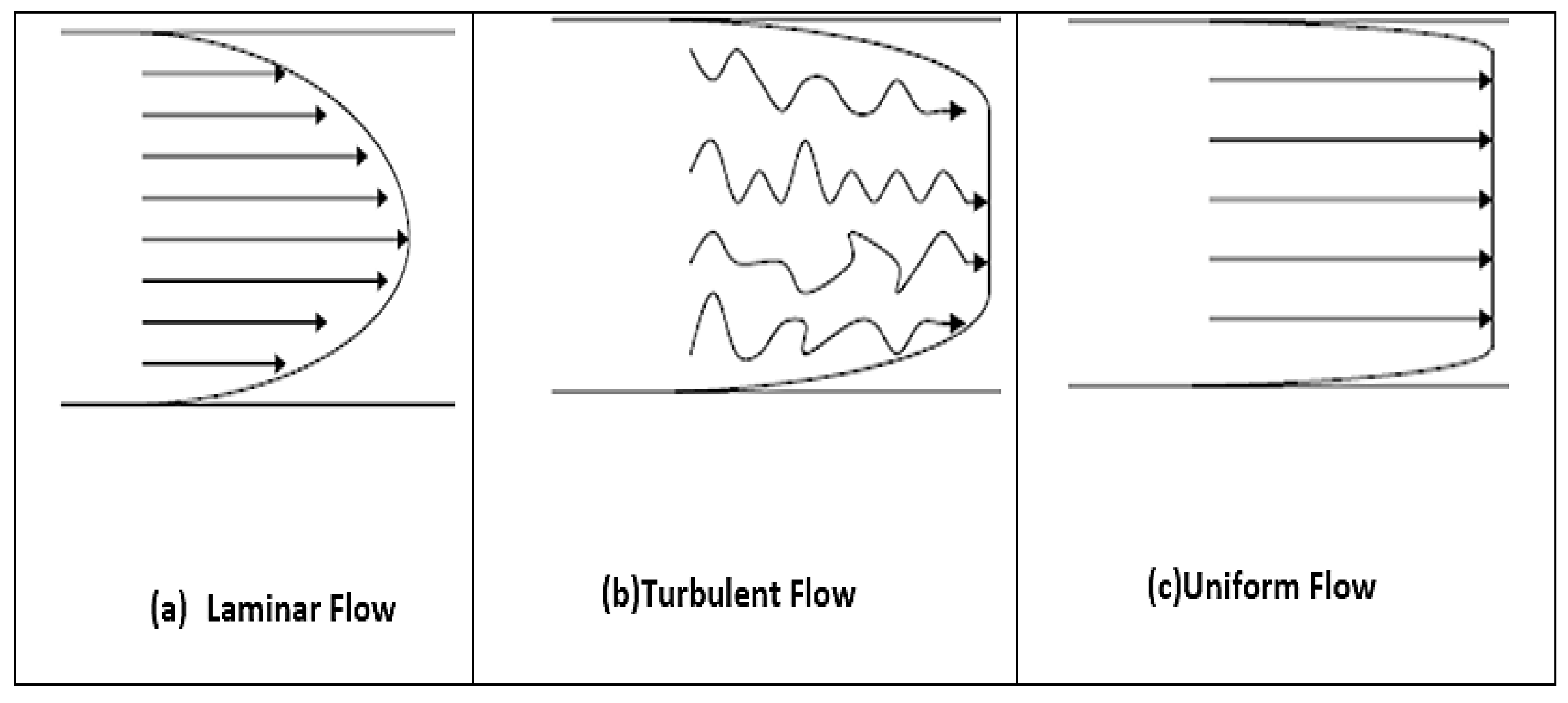
The laminar and turbulent flows have different profiles, as shown in Figure 2.

It is extremely unlikely that blood can enter turbulent flow under natural circulation conditions. Only severely stenosed vessels, extremely abnormal flow paths, and even certain pathological disorders that impair blood flow properties cause this. Non-Newtonian fluids have a flatter profile toward the axes, so the formed profiles are different. Blood appears to have a uniform velocity profile rather than a developed profile because of the diverse flow paths and irregular sizes of arteries [28,29].

2.3.4. Assessment of the Rate of Severe Stenosis

The amount of cross section that is “blocked” by occlusion determines the degree of stenosis. The narrowest segment (called “groove”) of the blockage is usually considered the cross section for stenoses with variable geometry. Figure 3 depicts a common model of a tube with a single stenosis in which the original radius of the vessel R0 is obstructed by a stenosis with a normalized maximum height of value = h/R₀, where h is the maximum height of the stenosis. To obtain the unit length, the available radius, R₀ = 1. Because the standardized height of the stenosis must be 0 ≤ δ <1, we can deduce the following [23].

The normalized cross section of light through CD = π

The normalized cross-section of light on AB = π (1 − δ)²

Thus, the percentage of blocked area can be derived; therefore, the severity of the stenosis is obtained as follows:

$$\frac{\mathsf{\pi }-\mathsf{\pi } {\left[1-\mathsf{\delta }\right]}^{2 }}{\mathsf{\pi }}\times 100\% =(1-{\left[1-\mathsf{\delta }\right]}^{2 })\times 100\%$$

(12)

3. Design and Description of the Solution Methodology

In this section, we apply our solution’s architecture and general technique, which includes the use of the Navier–Stokes equation in 2D to determine the action of blood fluid in a 3D model. Figure 4 shows the steps of each component of the solution, as well as an overview of the advantages of using CFD modules and the methods used. Our benchmark is composed of three parts, as indicated in Figure 4:

1—3D Medical Image Processing Software and Mimics Innovation Suite and Materialize for export, import, and management of 3D modeling of the stenosing aorta format;

2—ANSYS Fluent for computational fluid dynamics (CFD) manipulation and fifth dimensional “flux” modeling;

3—MR 4D Flow data for the visualization of aortic blood flow as streamlines, pathlines, and color-coded vectors with Pie Medical Imaging stands for expertise in cardiovascular quantitative analysis software (confirmed to have stenosis by human experts).

Figure 4. Benchmark of 5D solution.

Figure 4. Benchmark of 5D solution.

The main purpose of CFD is to solve the problem by discretizing the paradigm into small cells. The CFD process is divided into three stages. The first phase is pre-processed. The domain of the study is defined and generated during this step, and the flux regions are discretized to form a mesh of cells. Better findings would be obtained with a finer mesh, but this would require more processing capacity. Several codes now have methods for adapting meshes after multiple iterations to obtain more precise meshes, if desired. The properties of the fluid, as well as any other phenomenon to be investigated, are evaluated at this level.

It is essential to develop the required boundary conditions for the model until the medium begins, and the equations that need to be solved are determined. This is achieved by adding known or controllable values to the nodes or cells along the domain boundary. These limit values can be used to evaluate the solution for the remainder of the fluid velocity. It is projected that defining the domain geometry and creating the grid would take up more than half of the time spent on a CFD project. Although current software has made this move simpler, rational skills and knowledge are needed to build real-world meshes and provide correct answers without using more computing power than is appropriate. In the second step, the mesh generated in the previous step is solved. Assigning an initial value to cells first initializes the model and performs preliminary assessments of solution techniques. The final stage is post-processing, which involves extracting and analyzing the data produced in the previous step. Rather than exporting raw data, today’s commercially available applications aim to improve the accessibility of the findings by optimizing visual appearance and data manipulation. This provides a graphical user interface that can depict geometry and grid, vector displacements, contour and surface tracing, particle detection, and other features based on the needs of the user. This move often requires fundamental knowledge to understand these findings.

4. Tools for 5D Imaging

To meet the increasing need for CFD in industrial applications, several businesses have created a variety of applications. To satisfy the existing demands of search and processing resources, the simulation capabilities as well as the user interface have been greatly enhanced.

ANSYS (https://www.ansys.com/products/fluids/ansys-fluent, accessed on 21 November 2021 (Academic and Professional version of Enterprise)), which is still one of the most widely used commercial codes for structural research, has also played a key role in the establishment of a package in the market. The benefit of this program is that it allows multiple supported programs to run on a single platform and be connected to one another. This was initially designed to provide developers with a single board on which they could construct a product from the ground up, validate it, and refine it. This includes constructing the target model, discretizing it into finite elements, running the requisite models, supplying the required data, and optimizing the model based on the available data. The number of applications capable of running in this area grew in tandem with the market demand. Finally, in addition to basic structural models, a wide variety of mechanics are included, including fluid flow, electromagnetic, and thermal [30,31,32].

We used the product of Pie Medical Imaging “Caas MR 4D Flow” (https://www.piemedicalimaging.com/product/mr-solutions/caas-mr-4d-flow/, accessed on 21 November 2021 (Private access to the user with a procuration of agreement for the use of the product)) to analyze the valve behavior, considering the difficulty of the reconstruction of the valve structure from the flow sections. This cardiovascular solution aims to analyze blood flow in cardiovascular structures. Blood flow can be evaluated using three-way phase-contrast MRI images and the corresponding MRI images. In addition, blood flow can be analyzed by retrospective reformatting of flow planes. Caas MR 4D Flow is software that allows a cardiologist or radiologist to imagine and analyze blood flow in cardiovascular systems using multi-slice and multi-MRI images. It uses MRI and speed-coded images to examine blood flow in the heart and large arteries, and it contains the following features: analysis of quantitative cardiovascular results, segmentation of cardiovascular structures, and simulation of the intensity and direction of blood flow.

Whenever Caas MR 4D Flow findings are used in a clinical setting to sustain diagnosis, they should not be considered as the only compelling basis for clinical decision making.

5. Methods and Materials

For a 10-year-old patient with a history of congenital valve and valvular aortic stenosis on close MRI and coarctation (operated and then dilated) in the sense of shone syndrome, 74 cardiac MRI scans and 3057 images were obtained. Technically, reconstruction and segmentation of the descending aorta were performed using the following:

✓

44 TRICKS angiographic slices in dynamic acquisition on the thoracic aorta;

✓

Injection perfusion sequences after injection;

✓

Sequences ciné-fiesta T2 short-axis 4 cavities;

✓

Subsequent infusion sequences short-axis.

Clinical Diagnostic Report of LV:

For the ascending thoracic aorta without parietal abnormality, its main measurements are as follows:

✓

Tricuspid valve. Aortic ring with 8.5 mm diameter;

✓

Aortic stenosis at 0.42 cm² with reduction of sigmoid opening at 5 mm;

✓

At the sino-tubular junction: 25 mm;

✓

1/3 medium of the ascending aorta: 18 mm;

✓

Horizontal aorta: 16 mm;

✓

Size disparity with aortic stenosis at the isthmic level extended over 10 mm, reducing approximately 65% of its lumen by 6 mm in diameter;

✓

Mitral valve of normal diameter 2.5–4.3 cm²;

✓

The mass of VG tele-diastolic 90 g and tele-diastolic 70 g;

✓

The systolic ejection function, estimated according to the 82% contour method.

Features of TRICKS cuts and acquisition protocols:

✓

Magnetic field: 1.5 Tesla;

✓

Acquisition time: 1.2 s/Repetition time: 3.3 s;

✓

Diameter of reconstruction of the cuts: 370 cm²;

✓

Angle of acquisition = 30 degrees;

✓

Acquisition matrix: 0/300/224/0;

✓

Sections orientation matrix: −0.0393457\0.99917\−0.0105243\0.283665\0.00106985–0.958923;

✓

Cutting position matrix: −1.15748\−152.042\358.794;

✓

Number of time positions: 12;

✓

Scanning Rentals: −43.95322037;

✓

Space between pixels: 0.7227\0.7227 with allocation of 16 bits of memory.

6. Results

6.1. Model of the Geometry of the Descending Aorta in 3D

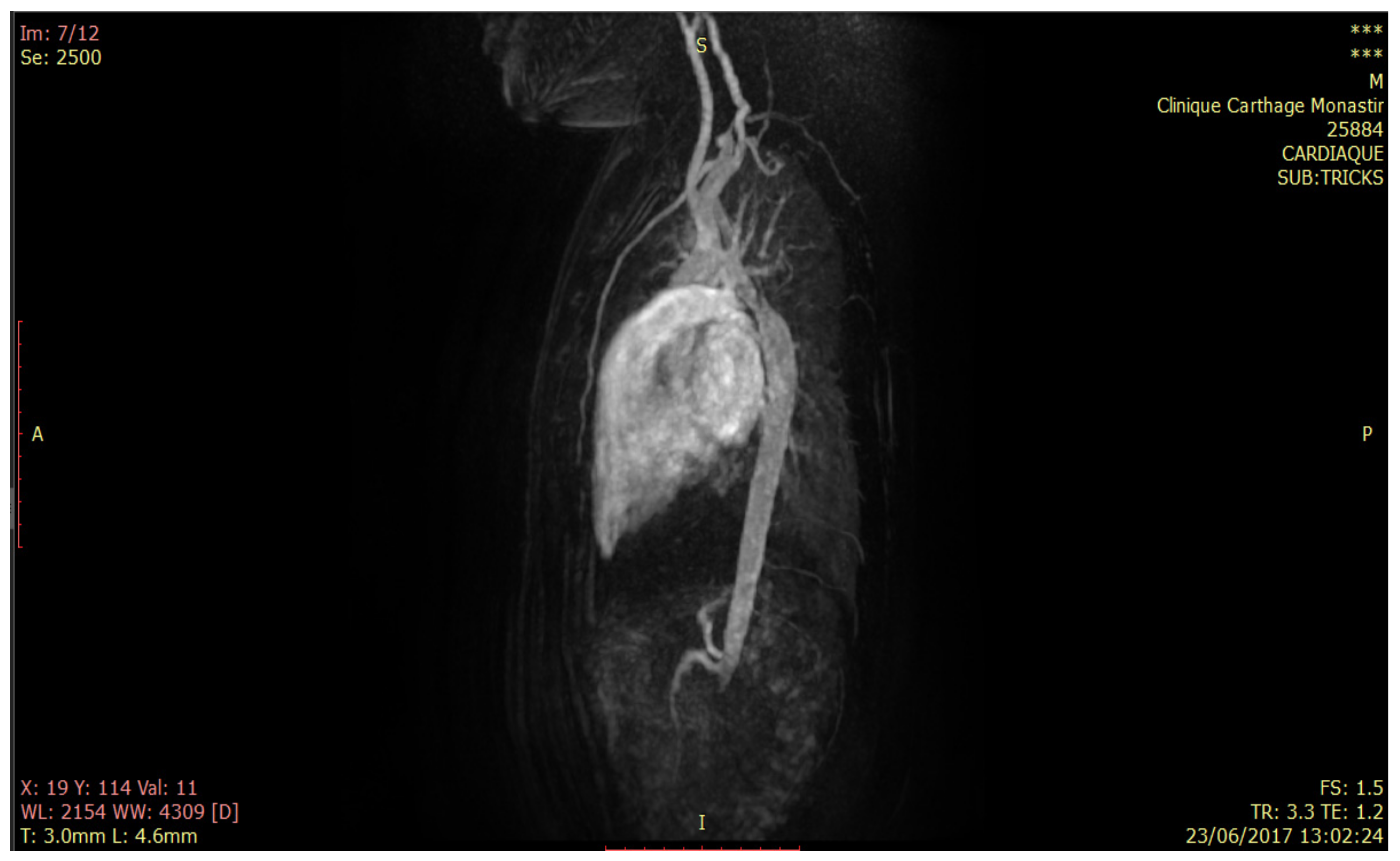
In this section, we proceed to the first phase of our 5D model, which consists of defining the geometry of the descending aorta in 3D. This step states the reconstruction of the aortic model from the TRICKS sections, as shown in Figure 5.

The multiplanar reconstruction in Figure 6 is a crucial step in the 3D reconstruction of the descending aorta presented in the axial plane in Figure 7.

We applied a threshold to the areas of interest to define the active mask. It was applied based on a low limit and a high limit. The mask contained pixels with a value between two threshold limits. The upper and lower thresholds were limited to the maximum and minimum intensities, respectively. We present the concept of the generic algorithm in

Table 2. Algorithm of thresholding.

Main steps of Algorithm

✓  Mask (Aorta Segment Mask)—Threshold Mask.

✓  Threshold_min (int)—Minimum threshold value :226

✓  Threshold_max (int)—The maximum value of the threshold: 1634

✓  Bounding_box (Aorte.BoundingBox3d)—(optional) Bounding box including region of interest

as follows.

Based on the detailed mathematical concept of [33], the thresholding is typically used in scans where a certain anatomy has a very distinct set of values (high contrast). Keeping only certain values of the medical image allows us to visualize the border of the aorta; in our case, the minimum and maximum threshold values were determined automatically. The threshold value for Mimi was approximately 270 (Hounsfield scale). A green mask was created after thresholding. The minimum threshold value for this case was 1235 (grey values) or 211 (Hounsfield values). Thresholding needs to be done before region growth since all previous work is lost after changing the threshold value.

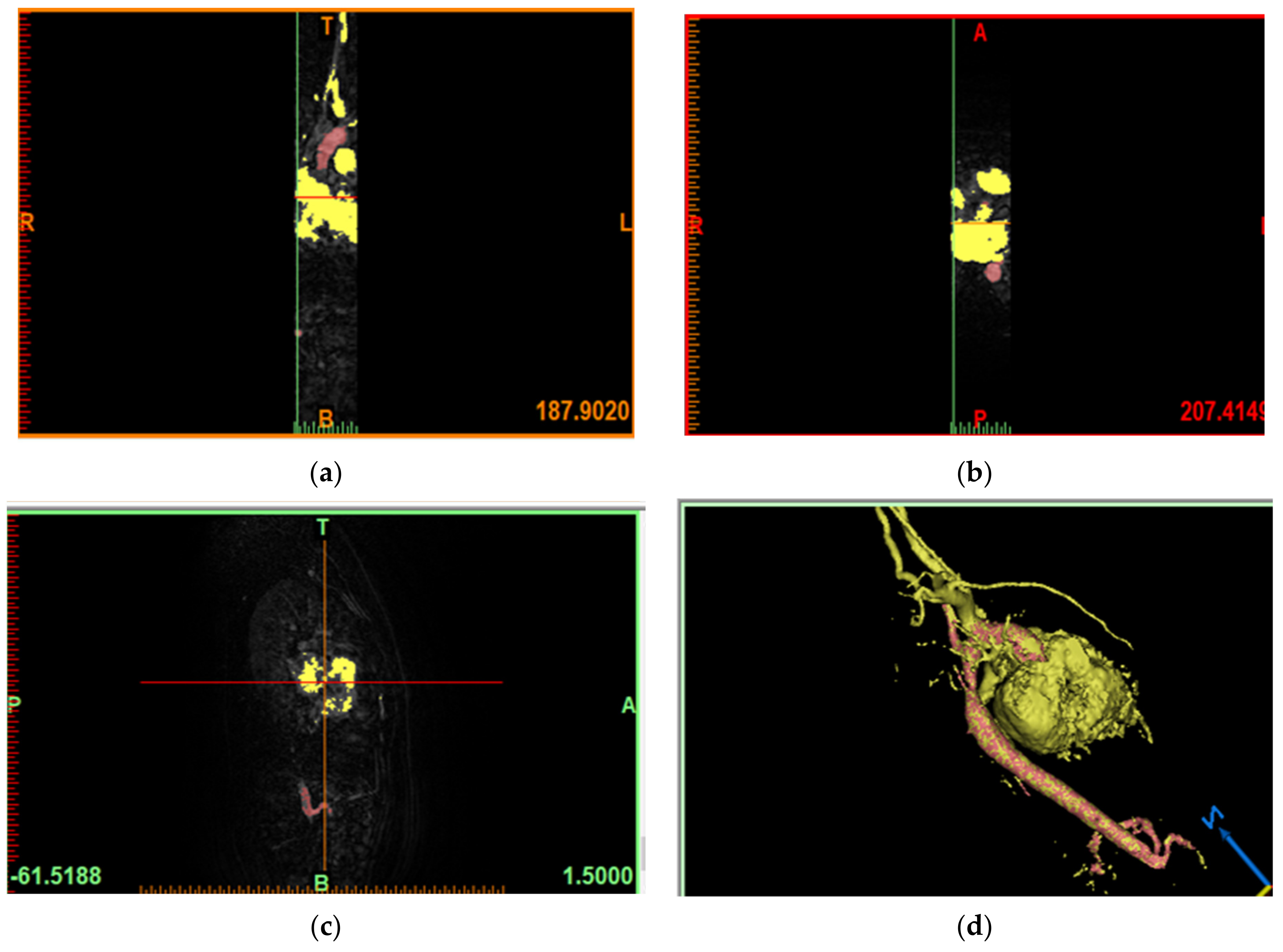
The updates according to the defined limits give a reconstruction of the model of the aorta in 3D based on the multiplanar reconstruction of the TRICKS cuts in Figure 8.

The second step was to divide the single mask for the entire model into two separate masks. This tool allows easy and fast separation of anatomical parts, such as the anatomical model of the heart and aorta. Two masks with the region of interest must be created and used as inputs to divide the selected mask, as shown in

Table 3. Algorithm of the mask application.

Main steps of Algorithm

✓  Selection (model.segment.Mask)—The original mask.

✓  Region_a_mask (model.Segment.Mask)—Existing mask containing marked regions to be separated from others. Region_a_mask takes precedence over region_b_mask.

✓  Region_b_mask (model.Segment.Mask)—Existing mask containing marked regions that must be separated from others. Region_a_mask takes precedence over region_b_mask.

✓  Model.segment. Calculate_part (mask, quality = ‘Optimal’)

.

We chose for the geometry calculation the “optimal” quality, partly corresponding to the input mask and custom parameters. The last step of this section was to clean the waste generated by the 3D reconstruction, as well as the smoothing and refining of the aorta model presented in Figure 9.

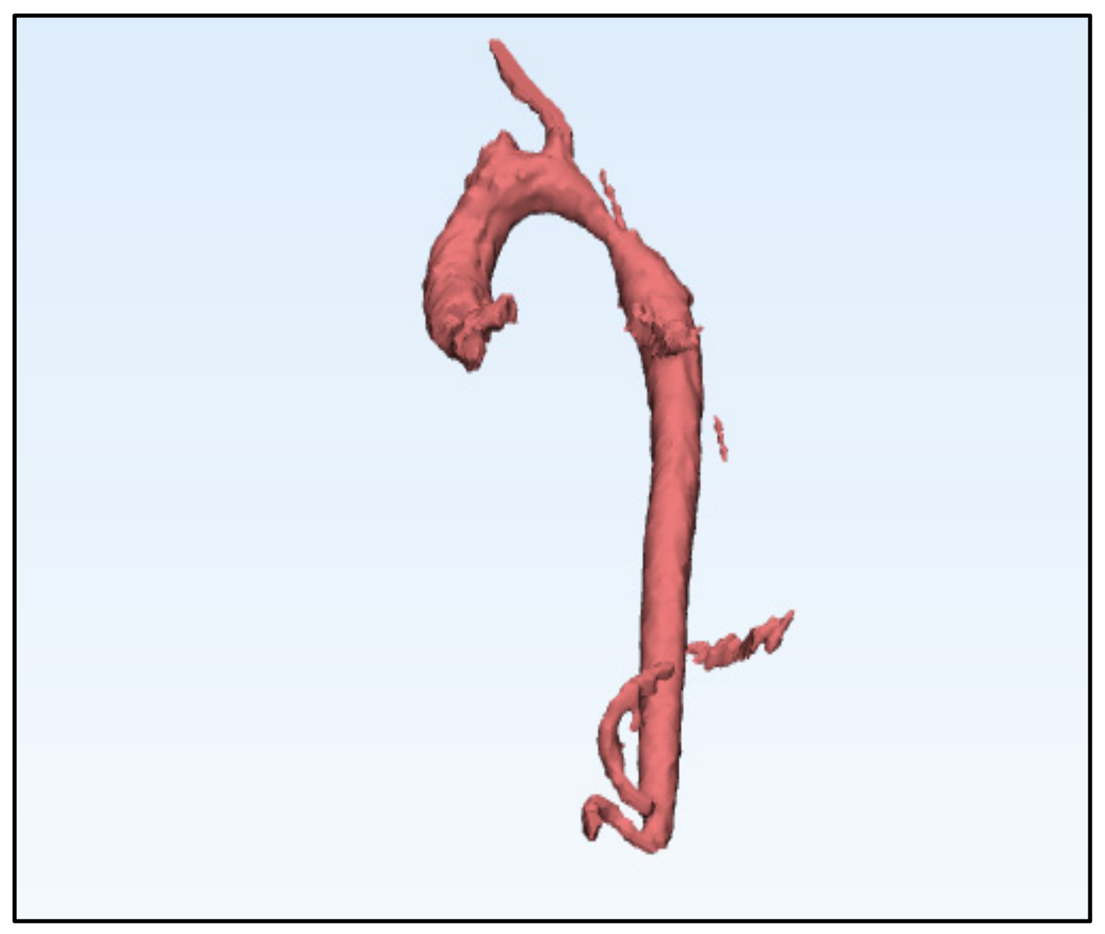
The best is that the accuracy of the three-dimensional reconstructions obtained depends essentially on the conditions and quality of acquisition of cuts, thickness of the cuts, distance between two successive acquisition slices, and the quality of the segmentation and the reconstruction algorithm used. The final geometry is shown in Figure 10.

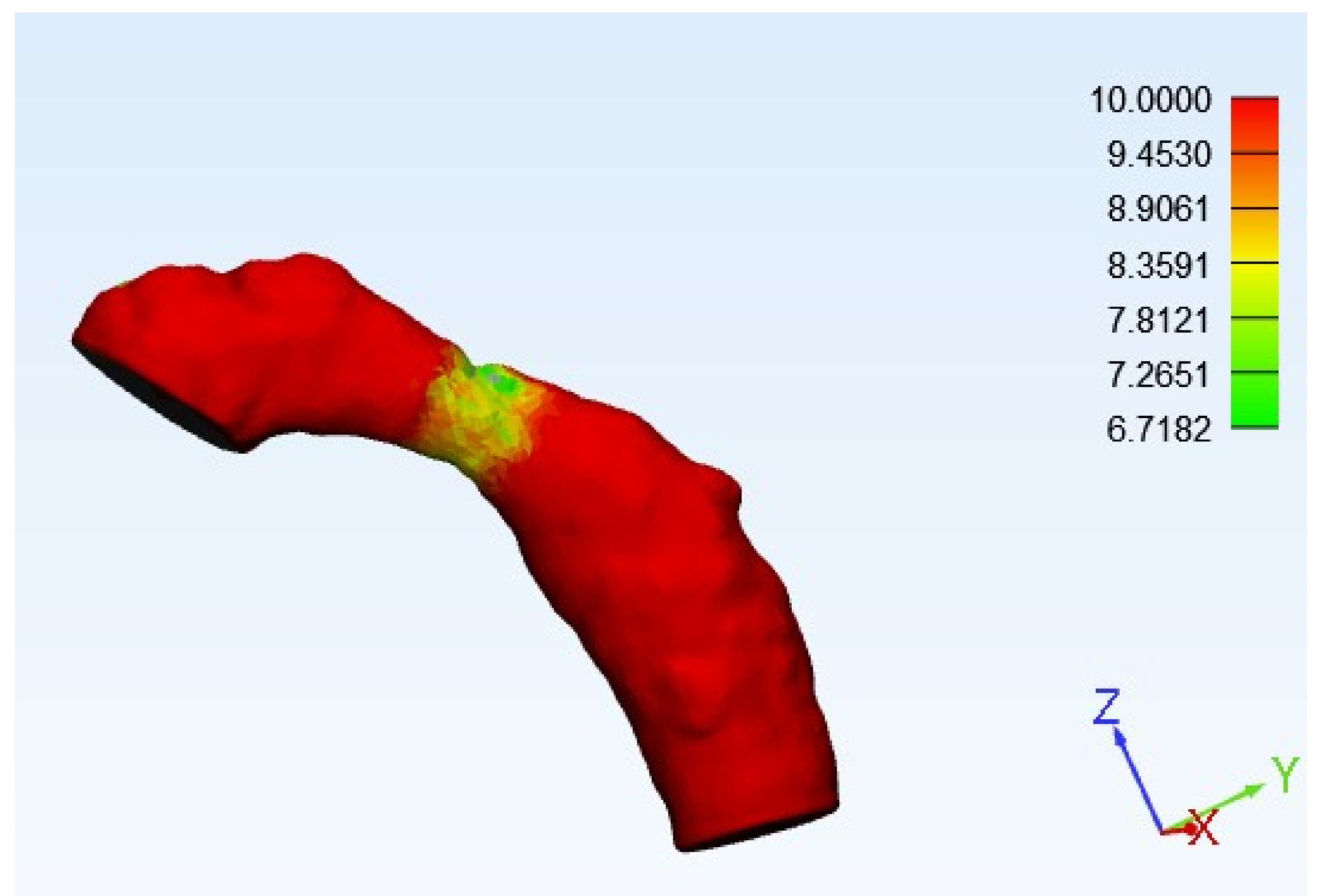
Based on a few statistical measures in

Table 4. Statistical analysis of the thickness and local curvature of the aorta.

Features	Statistical Analysis
	Based on the Thickness	Based on Curvature
Min-Edge	1.76 mm	3503.046
Max Edge	10 mm	6265.35
Median	10	0.09
Average	9.78	2.06
Standard Deviation	0.78	134.66
Average quadratic	9.81	134.67

, it can be seen that the thickness analysis presented in Figure 11 of the aorta can identify the stenosing portion of the aorta.

Note that the local curvature, as shown in Figure 12, of the segment that contains the shrinkage takes negative values. At this stage, the surface deformation as well as the measure of local curvature can be useful indices for aid in diagnosis.

Based on the study in Section 2.3.4, the height of the obstacle, h, is calculated in

Table 5. Estimation of the degree of aortic stenosis.

Height (mm)	Radius (mm)	Normalized Height of the Stenosis (δ)	Rate of Stenosis (%)
0.618	6.718	0.091991664	17.6%
0.337	7.265	0.046386786	9.1%
0.057	7.812	0.007296467	1.5%
0.223	8.359	0.026677832	5.3%
0.504	8.9	0.056629213	11.0%
0.784	9.4	0.083404255	16.0%
1.065	10	0.1065	20.2%
Estimated occlusion rate			80.5%

with respect to the unobstructed radius, which gives δ in Equation (13) a value of the severity of the stenosis to each part of the segment of the aorta.

6.2. Generation of the Mesh Geometry

In this section, it is crucial to prepare a proper format for the aortic geometry to proceed to the mesh operation. The 3D model was transformed into a geometric smoothing (IGS) format to divide the entire volume into facets that contain triangles, edges, and intersection nodes. This IGS export approach is used to process surface-based functional data, primarily to recreate functions from noisy observations. The proposed IGS method has a broad range of applications, especially in industrial settings. Based on the simulations, the IGS appears to be similar to other commonly used CFD processes. The mathematical modeling and simulation environment presentation is detailed by [34] with precision analysis for IGS models described by [35]. The second phase consists of decomposing the IGS model into three elements, the body, inlet, and outlet, as shown in Figure 13.

The geometry of the stenosing aorta has the following characteristics: length along the x-axis = $3.6339 \times {\mathrm{10}}^{-2} m$ length along the y-axis = $5.66596 \times {\mathrm{10}}^{-2} m$, length along the z-axis = $8.4559 \times {\mathrm{10}}^{-2} m$ with a total volume = $2.5915 \times {\mathrm{10}}^5 m^3$ number of nodes = 593,223, and number of elements = 3,168,417. The inlet edge field contains 32 faces with an area of $2.6563 \times {\mathrm{10}}^{-4} m^2$.

The outlet field contains 41 facets with an area $\mathrm{of} 4.0045 \times {\mathrm{10}}^{-4} m^2$. The number of faces of the body (wall) is 449, with a total area of $5.6453 \times {\mathrm{10}}^{-4} m^2$. The results of the mesh are shown in Figure 14.

6.3. Setting of the Solution

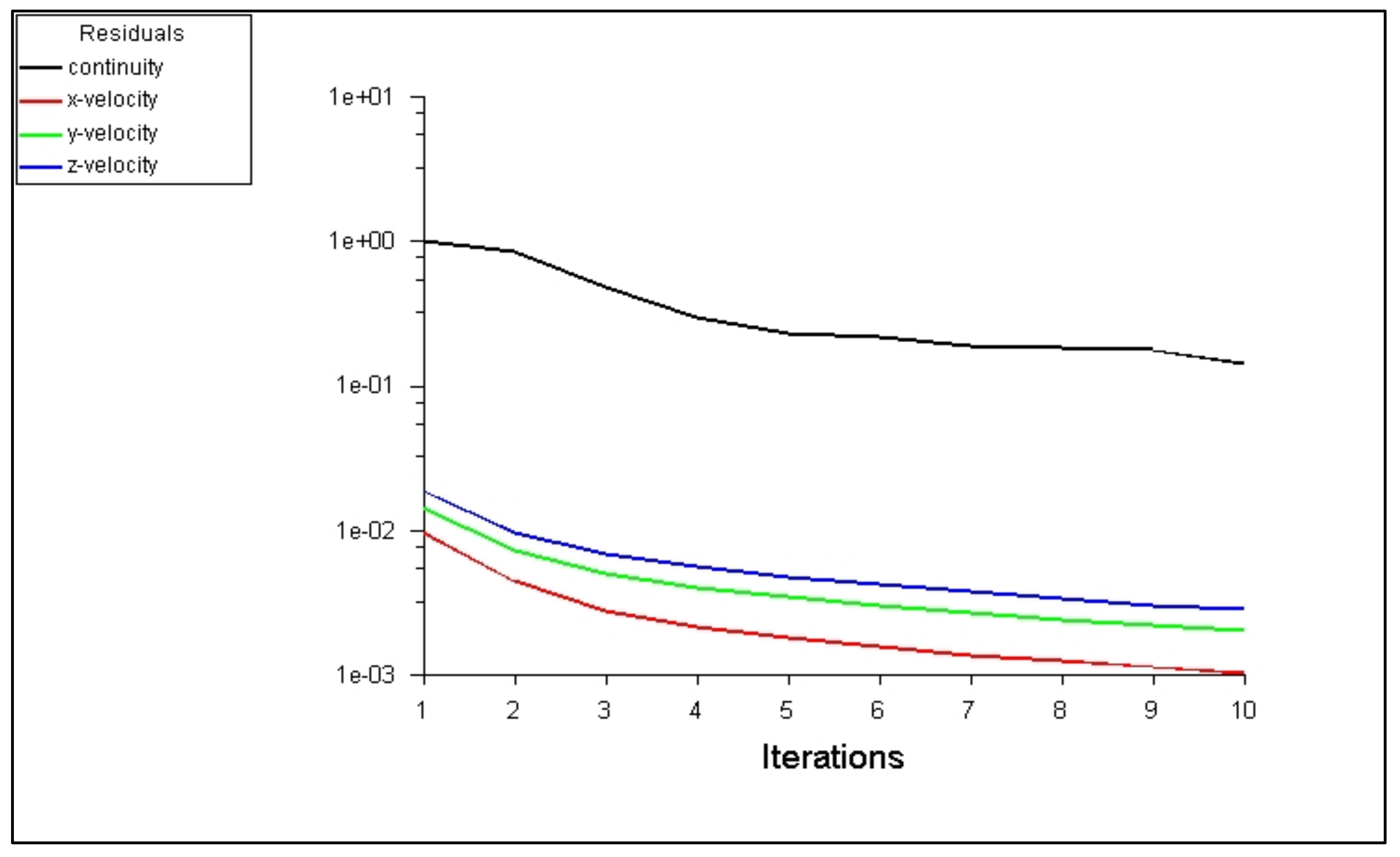
To solve the 2D Navier–Stokes equation, the configuration of this fluid solver is based on the pressure with absolute velocity formation in a stable time. Our fluid is blood with a density of 1056 (kg/m³) and a viscosity of 6 (kg/m³). The boundary condition must be zero for the aortic model. The execution of the laminar flow model defines the velocities and pressure in the viscous flow field (the Navier–Stokes equation) to solve the displacement of the internal facet of the 3D model of the aorta. During the resolution during the first 10 iterations, the velocity residuals along the three axes (x, y, z) are estimated in Figure 15.

The dimensions of velocity and pressure are combined in the momentum that governs the fluid equations. The coupled and independent methods are the two primary methods for solving discrete time equation algebraic equations. The simultaneous solution of the velocity and pressure parameters characterizes a coupled system. However, it is not commonly used in technical problems, owing to its poor processing power and high memory requirements. Coupled methods are commonly used for calculating compressible flows, whereas separate methods are favored for calculating incompressible flows. Unlike a coupled solution, a single approach solves the velocity and pressure fields independently or sequentially. It has the benefit of reducing computer memory and processing time, making it more effective for studying incompressible environment simulation fluids, as in our case for aortic stenosis modeling [36]. The pressure analysis of the proposed model is shown in Figure 16.

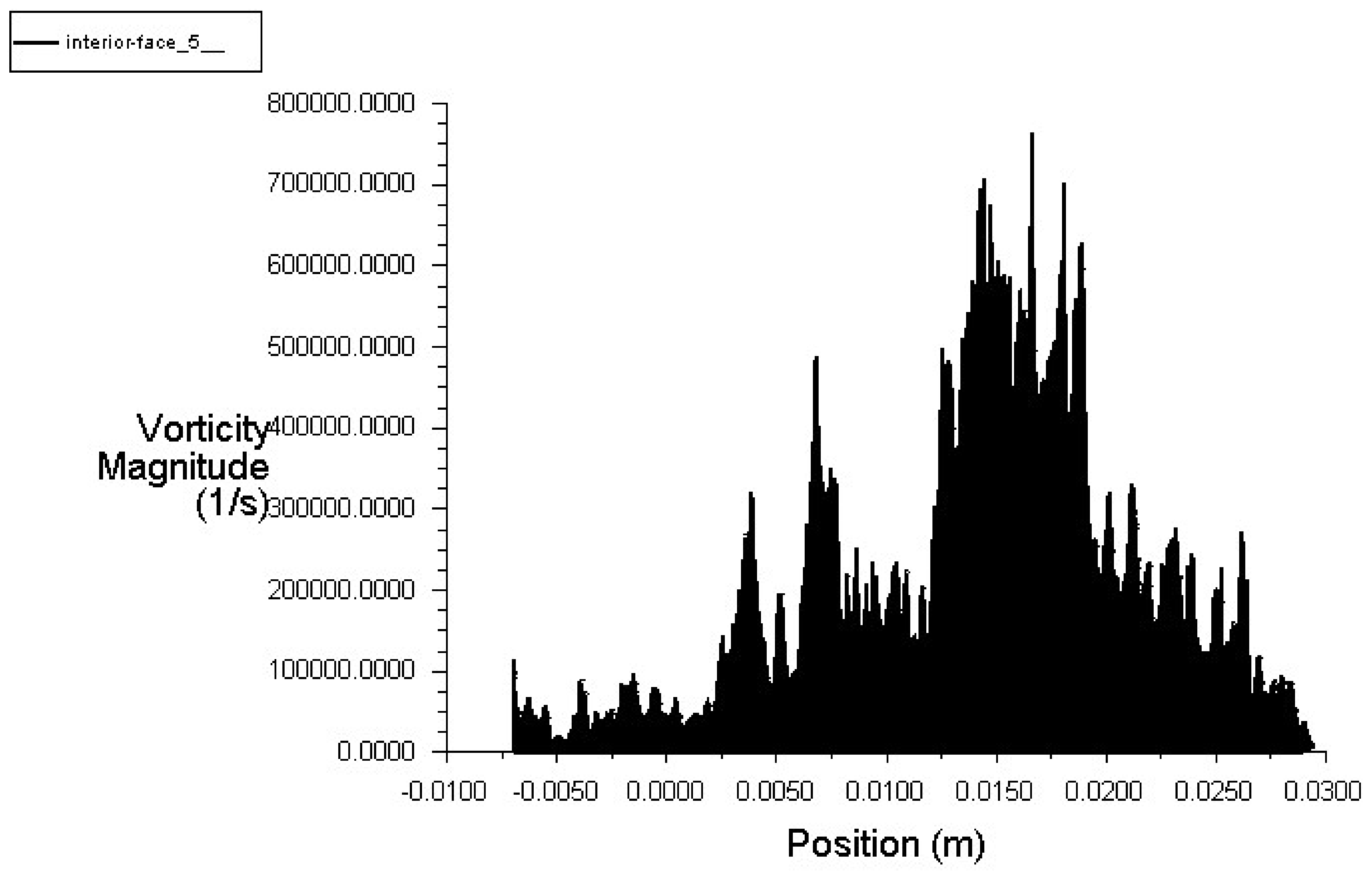
From this illustration, it can be concluded that the pressure at the entrance and exit is negligible compared to the body outside and inside the model of the stenotic aorta. The pressure intersection (Pa) between these two zones (inside and outside) of the wall at a critical point at a position of 15 mm shows a remarkable overlap between the red and blue parts, which explains why turbulence can occur because of the strength of the parietal wall exerted by the external and internal body. The location of blood flow in a case of aortic dissection with a complicated geometric feature, qualitatively and quantitatively, based on the evolution of vortex structures and their interaction in the narrowing region throughout a cardiac cycle can provide an index of the presence of stenosis from a 15 mm length of the aortic segment. A vortex field simulation in the wall of the internal aorta is shown in Figure 17 as well as the flow rate mass in Figure 18 to evaluate the vortex behavior.

We deduced from these two results that at the position of 15 mm, there is a very high vortex magnitude that reaches (800,000 (1/s)) as well as a mass of negative fluxes during the first six iterations during the solver calculation. This reflux shows that it occludes a segment of the aorta. These indices support the results reported in the clinical assessment with isthmic extensor aortic stenosis extending over 10 mm in length, reducing approximately 65% of its lumen by 6 mm in diameter, compared to what we estimated to be a 15 mm wide aortic stenosis; a 5 mm error rate was detected.

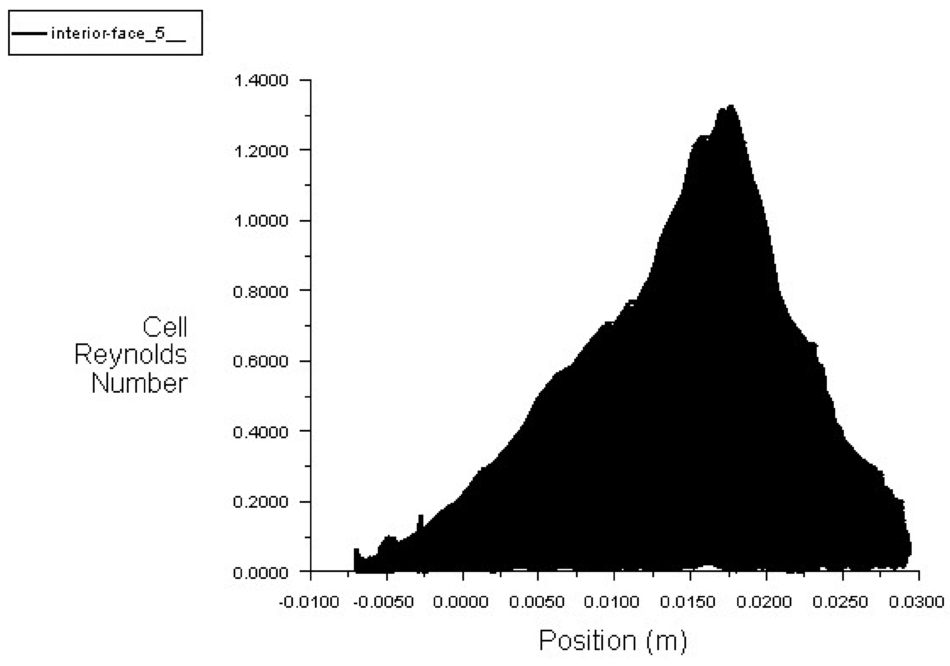
Owing to the very small size of the geometry, the Reynolds number is small enough for the laminar flow that appears throughout the aorta model, as shown in Figure 19. In our case of aortic coarctation, the highly disturbed flow areas exhibited Stokes flow characteristics. The friction factor, vortex length, shear stress, leakage flow strain, and turbulence results obtained with the low-Re turbulence model were compared with experimental data and findings achieved in terms of velocity profile, vortex length, shear stress, and turbulence.

Because of the unfavorable pressure gradient produced in the expanding segment of the stenosis tube, downstream flow separation was observed, and its size increased with the Reynolds number. The wall shear stress along the stenosis aorta peaked at the stenotic throat, and the tip was notably lower for a longer stenosis. The critical Reynolds number at which the blood flow becomes transient or turbulent distal stenosis was accurately predicted using this model. More surprisingly, the vortex length measured with the formula (Low-Re) nearly matched the vortex length expected by laminar flow modeling on the Re spectrum of the laminar flow. The constant flux was caused by the low Reynolds number.

The flow becomes unstable at a relatively high Reynolds number. Finally, the analysis clearly shows that the proposed model is appropriate for studying blood flow in specific occlusion zones [37].

6.4. Solution with ANSYS-Fluent

The average size of the stagnation and shunt zones was predicted by CFD, but the length of the current line and the variations in speed due to aorta flow were underestimated. However, for quantitative confirmation of CFD findings and the quest for flow effects, such as tortuosity and laminar flow behavior, the measurement accuracy must be increased. At almost the same time, the CFD simulation effects are represented not only in terms of pressure drop, but also in terms of vector orientation and velocity, current lines, and regions of blood flow stagnation [38]. This time-based flow concept is used in the 3D modeling of the stenosing aorta to generate the 5D format shown in Figure 20.

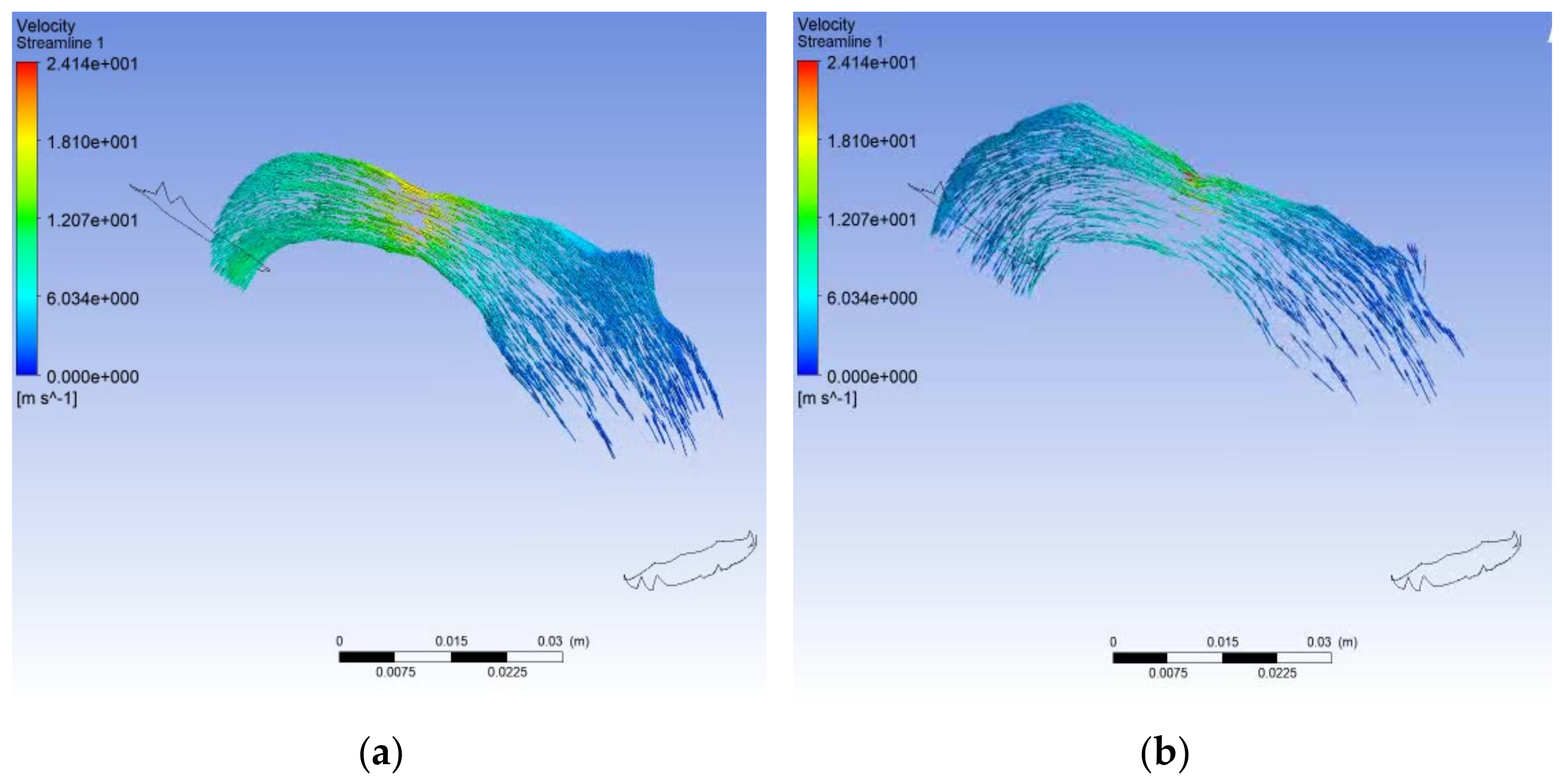
Owing to the fiber of this model, the fluid flow is deflected, resulting in a sinuous orientation of the flow lines, which shows a three-dimensional flow around the wall of the aorta, mainly directed from the inlet to the outlet. The area of stenosis in the middle, indicated by lower speeds, is shown in Figure 21.

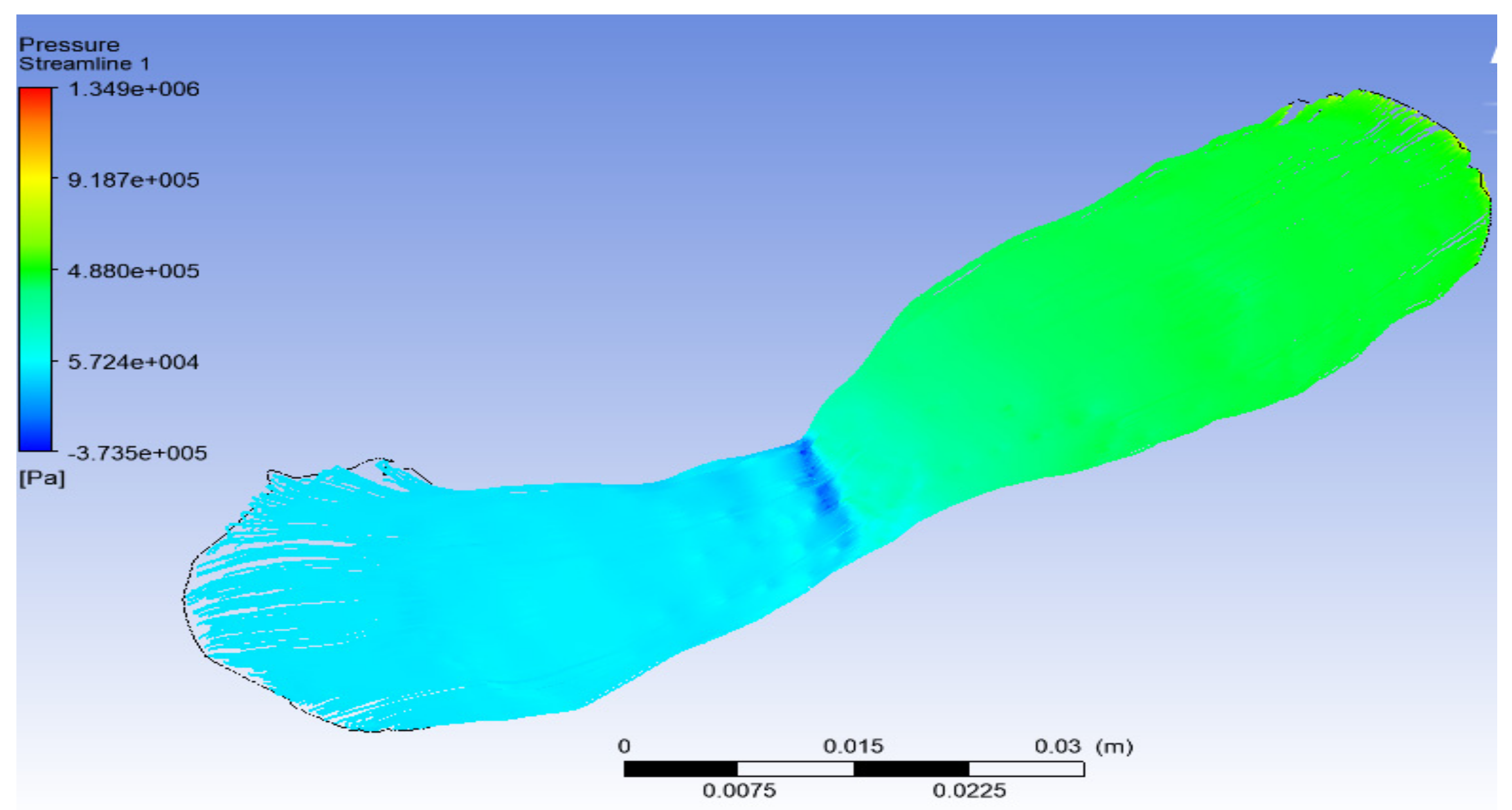
Focusing on the velocity in the stenosing part, we noticed that the flux field lines were delayed and decreased from 6.034 to 1.207 $\times {\mathrm{10}}^1$to $1.810\times {\mathrm{10}}^1 \left(m{s}^{-1}\right)$. Interestingly, the detection of negative pressure in the value narrowing zone was −3.735 $\times {\mathrm{10}}^5 \left[Pa\right]$, as shown in Figure 22.

6.5. Cardiovascular Solution with Pie Medical Imaging “Caas 4D Flow”

Our clinical case of aortic coarctation led to narrowing of the aortic valve with shone syndrome (two single-pillar valvular leaflet). In this case, the 5D model for the valve structure is corrosive, given the morphological dissection of the valve leaflet. The definition of the inputs and outputs, as well as the conditions of the limits of the aortic valve, are complicated because the valve acts as a blood pump. For this reason, the use of this research product that enhances the fifth dimension of 2D blood flow is used to predict and simulate the occlusion rate at the aortic valve level. Caas MR 4D Flow allows examining the 2D blood flow by reformatting planes in a 3D volume retrospectively. Additional plans can be placed on the 3D volume’s middle side. Standard 2D flow parameters, such as the flow rate, forward flow, and back flow, can be measured using 2D flow analysis. In addition, an extreme eccentric flow measurement in a plane was calculated based on the method of moving the flow [39]. The contour is redefined on its initial contour, initially shown by the Caas MR 4D flow in Figure 23.

The displacement of the flow is defined as the distance between the center of the light and the “center of velocity” of the flow, normalized with respect to the diameter of the light. The center of velocity (C_vel) was calculated as the average position of the pixels of the light (r_i, where i = x, y, z), weighted by the velocity information (v_i) as follows:

$${\mathrm{C}}_{\mathrm{vel},\mathrm{j}}=\frac{{\sum }_i{r}_{i,j}\left|v_i\right|}{{\sum }_i\left|v_i\right|}$$

(13)

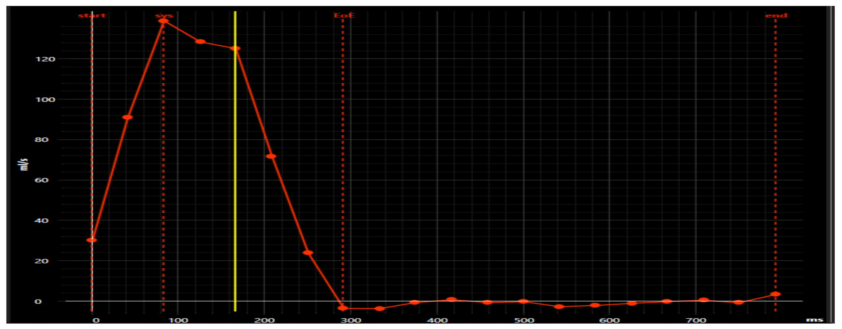
where i represents the pixels within the vessel’s outline, and j represents the spatial orientation of the pixels relative to the location of the center of the vessel. This method is described in more detail in the literature [39,40]. The flow displacement was calculated for the maximum systolic phase only, as shown in Figure 24. The maximum systolic phase was determined for each transmitter plane and determined using the time slot at the top of the 2D graph. The maximum systolic phase was indicated as a marker of phase slider. A description of the measurements is presented in

Table 6. Extraction of the measurements for the quantification of the fifth dimension of flow.

Anterograde flow (mL/beat)	25.56
Retrograde flow (mL/beat)	0.67
pumped blood (mL/beat)	24.89
Regurgitation fraction	0.03
Difference of pressure (mmHg)	14.96
Flow movement	0.08

.

Antegrade flow is used to quantify the blood pumped in the positive direction measured on the plane in a cardiac cycle, while retrograde flow is used to measure the amount of blood pumped in the positive direction on the plane in a cardiac cycle. The pump function of the valve was measured using forward flow to the back. The regurgitation fraction is the ratio of the backward flow (mL) to the forward flow (mL) and the area under the curve of the negative (backward flow) portion of the cardiac cycle. The gap between the vessel’s axis and the center of the eccentric flow was normalized to the total size of the vessel to enhance the heat transfer displacement [39]. It is possible to draw from this section the interest of studying the fifth dimension of blood flow to quantify and estimate both the regurgitation rate as well as a simulation of the minimum negative sign velocity of −81.4 (cm/s) to predict stenosis at the level of the aortic valve.

7. Discussion

A medical decision support method for cardiac imaging in MRI focused on 5D modeling (3D anatomical structure, temporal dimension, and blood flow dimension) for the study of a promising case of aortic coarctation with extreme valve narrowing was described. Our object of interest was a segment of the descending aorta for prediction, identifying the presence of aortic stenosis. The results show that in the first stage, the 3D modeling provides a very interesting index for the experts, which makes it possible to estimate the occlusion rate of 80.5% compared to what was manifested in the clinical assessment with a rate of 82%. The measurements extracted for the thickness and the local curvature with respect to the geometry of the aorta mark the zone of stenosis and the degree of deflection of the narrowing portion. In the second stage, the presentation of the 5D approach was performed through a combination of the 3D model and the size of the circulating blood flow as a function of time. The experiments that were performed for the fifth dimension provided high accuracy for the location of the stenosis zone of 15 mm in length compared to the clinical prognosis, indicating that aortic stenosis is extended over 10 mm, which is deduced from the solver of fluid (NS). During the first 10 iterations, a significant decrease in the flux mass was reported with −0.0050 (kg/s), as well as high blood turbulence in vortex field lines and low geometry Reynolds cells, which is based on the understanding and observation of a negative pressure value of $-3.735 \times {10}^5\left[\mathrm{Pa}\right]$. For negative velocity recognition (−81.4 cm/s), the fifth dimension was managed separately to assess velocity at the aortic valve with shone syndrome.

8. Conclusions

An approach for diagnosing medical decisions using cardiac imaging with MRI was described previously. This method necessitates the creation of a 5D model, which is composed of five dimensions: the anatomical structure of the heart in 3D, temporal dimensions, and a functional dimension of blood flow for the diagnosis of valve stenosis. A comparative study of practical technologies that leverage the fifth dimension of flow for the derivation of medical inference in clinical routine was also included. This contribution was studied for an aortic stenosis, and it comprised creating a 3D model and solving the Navier–Stokes equations for laminar and viscous blood fluid to arrive at the proposed 5D model (3D + time + flow). The region and degree of stenosis can be classified by extracting measures (vortex field, flow masses, static pressure, and Reynolds number) based on the fifth dimension. With the increasing need for high-resolution simulations, it is critical to investigate the cost and reaction time of digital solvers that could benefit from recent architectures, including multicore processors, in the future.

References

1. Solaiyappan, M. Visualization pathways in biomedicine. Handb. Med. Image Process. Anal. 2009, 729–753. [Google Scholar] [CrossRef]
2. Zhang, Y.; Passmore, P.; Bayford, R. Visualization and Post-processing of 5D Brain Images. In Proceedings of the 2005 IEEE Engineering in Medicine and Biology 27th Annual Conference, Shanghai, China, 17–18 January 2006; pp. 1083–1086. [Google Scholar] [CrossRef]
3. Brown, B.H.; Seagar, A.D. The Sheffield data collection system. Clin. Phys. Physiol. Meas. 1987, 8, 91–97. [Google Scholar] [CrossRef]
4. Wilson, A.J.; Milnes, P.; Waterworth, A.R.; Smallwood, R.H.; Brown, B.H. Mk3.5: A modular, multi-frequency successor to the Mk3a EIS/EIT system. Physiol. Meas. 2001, 22, 49–54. [Google Scholar] [CrossRef]
5. Rosset, A.; Spadola, L.; Pysher, L.; Ratib, O. Informatics in radiology (infoRAD): Navigating the fifth dimension: Innovative interface for multidimensional multimodality image navigation. Radiogr. Rev. Publ. Radiol. Soc. N. Am. Inc 2006, 26, 299–308. [Google Scholar] [CrossRef]
6. Cutrale, F.; Trivedi, V.; Trinh, L.A.; Chiu, C.-L.; Choi, J.M.; Artiga, M.S.; Fraser, S.E. Hyperspectral phasor analysis enables multiplexed 5D in vivo imaging. Nat. Methods 2017, 14, 149–152. [Google Scholar] [CrossRef]
7. Huang, Y.S.; Ku, H.Y.; Tsai, Y.C.; Chang, C.H.; Pao, S.H.; Sun, Y.H.; Chiou, A. 5D imaging via light sheet microscopy reveals cell dynamics during the eye-antenna disc primordium formation in Drosophila. Sci. Rep. 2017, 7, 44945. [Google Scholar] [CrossRef]
8. Vamvakeros, A.; Jacques, S.D.M.; Di Michiel, M.; Matras, D.; Middelkoop, V.; Ismagilov, I.Z.; Matus, E.V.; Kuznetsov, V.V.; Drnec, J.; Senecal, P.; et al. 5D operando tomographic diffraction imaging of a catalyst bed. Nat. Commun. 2018, 9, 4751. [Google Scholar] [CrossRef] [Green Version]
9. Heist, S.; Zhang, C.; Reichwald, K.; Kühmstedt, P.; Notni, G.; Tünnermann, A. 5D hyperspectral imaging: Fast and accurate measurement of surface shape and spectral characteristics using structured light. Opt. Express 2018, 26, 23366–23379. [Google Scholar] [CrossRef]
10. Low, D.A.; Parikh, P.J.; Lu, W.; Dempsey, J.F.; Wahab, S.H.; Hubenschmidt, J.P.; Nystrom, M.M.; Handoko, M.; Bradley, J.D. Novel breathing motion model for radiotherapy. Int. J. Radiat. Oncol. 2005, 63, 921–929. [Google Scholar] [CrossRef]
11. Sigfridsson, A.; Kvitting, J.-P.E.; Knutsson, H.; Wigström, L. Five-dimensional MRI incorporating simultaneous resolution of cardiac and respiratory phases for volumetric imaging. J. Magn. Reson. Imaging JMRI 2007, 25, 113–121. [Google Scholar] [CrossRef]
12. Feng, L.; Coppo, S.; Piccini, D.; Yerly, J.; Lim, R.P.; Masci, P.G.; Stuber, M.; Sodickson, D.K.; Otazo, R. 5D whole-heart sparse MRI. Magn. Reson. Med. 2018, 79, 826–838. [Google Scholar] [CrossRef]
13. Sakly, H.; Mahmoudi, R.; Akil, M.; Said, M.; Tagina, M. Moving towards a 5D cardiac model. J. Flow Vis. Image Process. 2019, 26, 19–48. [Google Scholar] [CrossRef] [Green Version]
14. Sakly, H.; Said, M.; Tagina, M. Computer Methods and Programs for Medical Decision Making: 5D Cardiac Model; Eliva Press: Chisinau, Moldova, 2020. [Google Scholar]
15. Sikarwar, B.S.; Roy, M.; Ranjan, P.; Goyal, A. Automatic disease screening method using image processing for dried blood microfluidic drop stain pattern recognition. J. Med. Eng. Technol. 2016, 40, 245–254. [Google Scholar] [CrossRef]
16. Roy, M.; Singh Sikarwar, B.; Bhandwal, M.; Ranjan, P. Modelling of Blood Flow in Stenosed Arteries. In Proceedings of the 7th International Conference on Advances in Computing & Communications, ICACC-2017, Cochin, India, 22–24 August 2017; pp. 821–830. [Google Scholar] [CrossRef]
17. Cebral, J.R.; Mut, F.; Raschi, M.; Scrivano, E.; Ceratto, R.; Lylyk, P.; Putman, C.M. Aneurysm rupture following treatment with flow-diverting stents: Computational hemodynamics analysis of treatment. AJNR Am. J. Neuroradiol. 2011, 32, 27–33. [Google Scholar] [CrossRef] [Green Version]
18. Thomas, B.; Sumam, K.S. Blood Flow in Human Arterial System-A Review. Procedia Technol. Int. Conf. Emerg. Trends Eng. Sci. Technol. 2016, 24, 339–346. [Google Scholar] [CrossRef] [Green Version]
19. Xiong, G.; Figueroa, C.A.; Xiao, N.; Taylor, C.A. Simulation of blood flow in deformable vessels using subject-specific geometry and spatially varying wall properties. Int. J. Numer. Methods Biomed. Eng. 2011, 27, 1000–1016. [Google Scholar] [CrossRef] [Green Version]
20. Cibis, M.; Jarvis, K.; Markl, M.; Rose, M.; Rigsby, C.; Barker, A.J.; Wentzel, J.J. The effect of resolution on viscous dissipation measured with 4D flow MRI in patients with Fontan circulation: Evaluation using computational fluid dynamics. J. Biomech. 2015, 48, 2984–2989. [Google Scholar] [CrossRef] [Green Version]
21. Holden, M. A review of geometric transformations for nonrigid body registration. IEEE Trans. Med. Imaging 2008, 27, 111–128. [Google Scholar] [CrossRef]
22. He, X.; Hu, W.; Zhang, Y. Observer-based feedback boundary stabilization of the Navier–Stokes equations. Comput. Methods Appl. Mech. Eng. 2018, 339, 542–566. [Google Scholar] [CrossRef]
23. Chan, W.Y. Simulation of Arterial Stenosis Incorporating Fluid-Structural Interaction and Non-Newtonian Blood Flow. Ph.D. Thesis, RMIT University, Melbourne, VIC, Australia, 2006. [Google Scholar]
24. Bakharev, F.L.; Exner, P. Geometrically Induced Spectral Effects in Tubes with a Mixed Dirichlet—Neumann Boundary. Rep. Math. Phys. 2018, 81, 213–231. [Google Scholar] [CrossRef] [Green Version]
25. Leuprecht, A.; Perktold, K. Computer simulation of non-newtonian effects on blood flow in large arteries. Comput. Methods Biomech. Biomed. Eng. 2001, 4, 149–163. [Google Scholar] [CrossRef]
26. Pereira, J.M.C.; Serra e Moura, J.P.; Ervilha, A.R.; Pereira, J.C.F. On the uncertainty quantification of blood flow viscosity models. Chem. Eng. Sci. 2013, 101, 253–265. [Google Scholar] [CrossRef]
27. Cengel, Y.A.; Cimbala, J.M.; Turner, R.H. Fundamentals of Thermal Fluid Sciences 5th Edition Cengel Solutions Manual. BASIC CONCEPTS Thermodyn. 2017. Available online: https://testbanklive.com/download/fundamentals-of-thermal-fluid-sciences-5th-edition-cengel-solutions-manual/ (accessed on 1 August 2018).
28. Nadeem, S.; Ali, M. Analytical solutions for pipe flow of a fourth grade fluid with Reynold and Vogel’s models of viscosities. Commun. Nonlinear Sci. Numer. Simul. 2009, 14, 2073–2090. [Google Scholar] [CrossRef]
29. Disu, A.B.; Dada, M.S. Reynold’s model viscosity on radiative MHD flow in a porous medium between two vertical wavy walls. J. Taibah Univ. Sci. 2017, 11, 548–565. [Google Scholar] [CrossRef] [Green Version]
30. Zaripov, T.S.; Rybdylova, O.; Sazhin, S.S. A model for heating and evaporation of a droplet cloud and its implementation into ANSYS Fluent. Int. Commun. Heat Mass Transf. 2018, 97, 85–91. [Google Scholar] [CrossRef]
31. Tora, E.; Dahlquist, E. CFD Ansys—Fluent Simulation of Prevention of Dioxins Formation Via Controlling Homogeneous Mass and Heat Transfer within Circulated Fluidized Bed Combustor. Energy Procedia 2015, 75, 130–136. [Google Scholar] [CrossRef] [Green Version]
32. Hosseini, S.A.; Vahedi Tafreshi, H. Modeling particle-loaded single fiber efficiency and fiber drag using ANSYS–Fluent CFD code. Comput. Fluids 2012, 66, 157–166. [Google Scholar] [CrossRef]
33. Dey, D.K.; Rao, C.R. Bayesian Thinking: Modeling and Computation; Amsterdam, The Netherlands, 2005; Available online: https://xueshu.baidu.com/usercenter/paper/show?paperid=8c0b82d85902b8be920dcaec170ffcc9&site=xueshu_se&hitarticle=1 (accessed on 20 December 2021).
34. Wilhelm, M.; Dedè, L.; Sangalli, L.M.; Wilhelm, P. IGS: An IsoGeometric approach for smoothing on surfaces. Comput. Methods Appl. Mech. Eng. 2016, 302, 70–89. [Google Scholar] [CrossRef] [Green Version]
35. Ray, J.; Rebischung, P.; Griffiths, J. IGS polar motion measurement accuracy. Geod. Geodyn. Geod. Astron. Geophys. Earth Rotat. 2017, 8, 413–420. [Google Scholar] [CrossRef]
36. Wang, H.; Wang, H.; Gao, F.; Zhou, P.; Zhai, Z. Literature review on pressure–velocity decoupling algorithms applied to built-environment CFD simulation. Build. Environ. 2018, 143, 671–678. [Google Scholar] [CrossRef]
37. Ghalichi, F.; Deng, X.; De Champlain, A.; Douville, Y.; King, M.; Guidoin, R. Low Reynolds number turbulence modeling of blood flow in arterial stenoses. Biorheology 1998, 35, 281–294. [Google Scholar] [CrossRef]
38. Schlanstein, P.C.; Hesselmann, F.; Jansen, S.V.; Gemsa, J.; Kaufmann, T.A.; Klaas, M.; Roggenkamp, D.; Schröder, W.; Schmitz-Rode, T.; Steinseifer, U.; et al. Particle Image Velocimetry Used to Qualitatively Validate Computational Fluid Dynamic Simulations in an Oxygenator: A Proof of Concept. Cardiovasc. Eng. Technol. 2015, 6, 340–351. [Google Scholar] [CrossRef]
39. Burris, N.S.; Sigovan, M.; Knauer, H.A.; Tseng, E.E.; Saloner, D.; Hope, M.D. Systolic flow displacement correlates with future ascending aortic growth in patients with bicuspid aortic valves undergoing magnetic resonance surveillance. Investig. Radiol. 2014, 49, 635–639. [Google Scholar] [CrossRef]
40. Sigovan, M.; Hope, M.D.; Dyverfeldt, P.; Saloner, D. Comparison of four-dimensional flow parameters for quantification of flow eccentricity in the ascending aorta. J. Magn. Reson. Imaging JMRI 2011, 34, 1226–1230. [Google Scholar] [CrossRef]
Figure 1. Modeling of the stenosing aorta.
Biomedinformatics 02 00002 g001
Figure 2. Velocity profiles for laminar (a), turbulent (b) and uniform (c) flow [9].
Biomedinformatics 02 00002 g002
Figure 3. The geometry showing the height of the stenosis, δ, initial radius of the vessel, R0 [9].
Biomedinformatics 02 00002 g003
Figure 5. Sample of TRICKS cuts for 2500 s of acquisition.
Biomedinformatics 02 00002 g005
Figure 6. Multiplanar reconstruction of TRICKS cuts for the aorta.
Biomedinformatics 02 00002 g006
Figure 7. Model of the descending aorta in axial plane.
Biomedinformatics 02 00002 g007
Figure 8. Reconstruction of the 3D model of the heart with the aorta. (a) Detection of the wall of the Aorta. (b) Detection of the inlet outlet of the Aorta. (c) Applying the Mask. (d) Reconstruction of the whole format of the Aorta
Biomedinformatics 02 00002 g008
Figure 9. A 3D aorta model with reconstruction waste.
Biomedinformatics 02 00002 g009
Figure 10. Final reconstruction of the descending aorta model in 3D.
Biomedinformatics 02 00002 g010
Figure 11. Thickness analysis of the aorta.
Biomedinformatics 02 00002 g011
Figure 12. Analysis of the curvature of the aorta.
Biomedinformatics 02 00002 g012
Figure 13. (a) Geometry of the aorta (a) in inlet (b), outlet (c) and wall (d).
Biomedinformatics 02 00002 g013
Figure 14. Mesh of 3D aorta.
Biomedinformatics 02 00002 g014
Figure 15. Calculation of velocity residues during the first 10 iterations.
Biomedinformatics 02 00002 g015
Figure 16. Calculation of static pressure for input of aortic model in 3D (inlet), outlet (outlet), model of aorta outside (wall), model of aorta inside (interior-face5).
Biomedinformatics 02 00002 g016
Figure 17. Magnitude field of the vortex in the aorta.
Biomedinformatics 02 00002 g017
Figure 18. Mass flow rate.
Biomedinformatics 02 00002 g018
Figure 19. Reynolds cell number presentation for 3D aortic model (internal wall).
Biomedinformatics 02 00002 g019
Figure 20. Model 5D of the aorta.
Biomedinformatics 02 00002 g020
Figure 21. Flow line visualization in the 5D aorta model (without the 3D inner wall). (a)velocity streamline (frame1). (b) velocity streamline (frame2). (c) velocity streamline (frame3). (d) velocity streamline (frame4).
Biomedinformatics 02 00002 g021aBiomedinformatics 02 00002 g021b
Figure 22. Pressure of the 5D model of the aorta (without the inner wall in 3D).
Biomedinformatics 02 00002 g022
Figure 23. Contour accuracy of the aortic valve.
Biomedinformatics 02 00002 g023
Figure 24. Simulation of flow within the aortic valve.
Biomedinformatics 02 00002 g024