A Machine Learning-Empowered Workflow to Discriminate Bacillus subtilis Motility Phenotypes

Abstract

Bacteria that are capable of organizing themselves as biofilms are an important public health issue. Knowledge discovery focusing on the ability to swarm and conquer the surroundings to form persistent colonies is therefore very important for microbiological research communities that focus on a clinical perspective. Here, we demonstrate how a machine learning workflow can be used to create useful models that are capable of discriminating distinct associated growth behaviors along distinct phenotypes. Based on basic gray-scale images, we provide a processing pipeline for binary image generation, making the workflow accessible for imaging data from a wide range of devices and conditions. The workflow includes a locally estimated regression model that easily applies to growth-related data and a shape analysis using identified principal components. Finally, we apply a density-based clustering application with noise (DBSCAN) to extract and analyze characteristic, general features explained by colony shapes and areas to discriminate distinct Bacillus subtilis phenotypes. Our results suggest that the differences regarding their ability to swarm and subsequently conquer the medium that surrounds them result in characteristic features. The differences along the time scales of the distinct latency for the colony formation give insights into the ability to invade the surroundings and therefore could serve as a useful monitoring tool.

1. Introduction

Biofilms are an emerging health problem, and knowledge discovery within the field remains an important topic for microbiologists that emphasize a clinical or hygienic perspective. It has been known for more than a century that colony morphology can be strikingly different between pathogenic and non-pathogenic strains of bacteria and should therefore be decisive in characterizing bacteria isolated from patients [1,2,3]. B. subtilis is a model organism for Gram-positive bacteria and is known for its different mobility, depending on the respective strain [4,5]. To access the characteristic phenotypic differences of the colony formation present in Bacillus subtilis, a set of wild-type and domesticated laboratory strains are used (see

Table 1. List of strains used in the study. * = flagella deficient. ∘ = Strain from the laboratory of Juan Alonso, Universidad Autónoma de Madrid.

Strain	Description	Reference
W3610	B. subtilis wild-type isolate	[9]
PY79	B. subtilis lab strain trpC2	[10]
PY79yhbEF	B. subtilis lab strain PY79, yhbEF::kan	[11] *
168	B. subtilis lab strain trpC2	[12,13]
BG214	B. subtilis lab strain	∘

). These strains are different regarding their ability to swarm and subsequently conquer the surrounding medium. Along time scales of distinct latency, colony formation gives insights into the strain-specific invasiveness. For instance, flagella-mediated motility is a physiologically important feature for many bacterial species, enabling them to effectively colonize new habitats [6]. Therefore, understanding bacterial motility is of key importance in the struggle for developing more efficiently conducted counteractive measures. In general, B. subtilis exhibits two forms of active flagella-driven movement: swimming, which refers to the movement of single cells in a three-dimensional space in liquid media, and swarming, in which cells assemble into rafts that move over a two-dimensional surface by joining their flagella forces. Swarming also relies on the secretion of a surface-tension-reducing compound [7]. Both behaviors can easily be monitored under laboratory conditions when cells are spotted onto LB agar plates with varying viscosity. At a concentration lower than 0.5 % agar, the swimming motility is predominant, whereas between 0.5 and 0.7 %, the swarming movement occurs [8]. Bacterial motility has been studied for a long time and is subject to several review articles (e.g., [7]).

The presented workflow is a framework to detect and analyze the strain-specific differences in their growth on solid agar plates based on simple gray-scale images in a reproducible manner. Given the empirical fact that a higher amount of biomass leads to an increased absorption of light, gray-scale images contain specific colony formation contours. After the initial thresholding, the contour information can be extracted and analyzed using regression models as well as a principal component analysis (PCA) prior to the application of a density-based clustering strategy involving noise. Considering the aspects mentioned above, the workflow (see Figure 1) of this study enables to monitor and model bacterial motility based on colony diameter growth over time. It is therefore hypothesized that a semi-automated machine learning workflow is capable of discriminating between phenotypes along the characteristics of varying motility and colony shapes.

2. Materials and Methods

2.1. Bacillus subtilis

B. subtilis is one of the best studied model organisms and one of the most important domesticated microorganisms. B. subtilis belongs to rod-shaped bacteria found in soils [15]. In terms of model organisms, B. subtilis is the Gram-positive and aerobic counterpart to Escherichia coli and is one of the most important species in industry mostly used for heterologous expression of recombinant enzymes or other products delivered by the organism. B. subtilis is very resistant to damage induced by electromagnetic radiation, detergents or other relevant damage and rapidly undergoes its survival state (spores). Furthermore, B. subtilis is known to form thick biofilms consisting of distinct cell growth-phase-dependent shapes along the local gradient of oxygen availability. It is known that strain W3610 produces surfactin and modulates the medium regarding its hydrophobicity, unlike strain 168 which expresses flagella only [16]. The biological model system in this study contains classes of distinct B. subtilis strains that are different regarding their ability to swarm or secrete specific bio-molecules (see Table 1).

2.2. Bioimaging Strategies

Cells are inoculated and cultured in lysogeny-broth (LB) [17] at 200 rpm/30 °C overnight. Overnight culture is transferred on LB agar plates to form colonies during another overnight incubation at 30 °C. Resulting colonies are used as a model to monitor growth pattern formation over days (see Figure 2) or hours, respectively, (see Section 2.2.2). Gray-scale images are acquired using common gel-illuminator setups used in almost every biochemistry-driven laboratory for camera-based investigation visualization of electrophoresis results, for instance, shown in Figure 2A,D. Cells are incubated at different time scales on an agar plate at 30 °C. Strain images of cell colonies are acquired sequentially according to different temporal scaling. For invasion/swarming curves, time lapse temporally resolves to hours whilst larger incubation times for colony formation resolve within days of incubation. According to that, the identified problem is a regression type. Therefore, non-parametric locally estimated scatterplot smoothing (LOESS) regression model [18,19,20] is used for invasion analysis of distinct B. subtilis phenotypes. Based on a custom FIJI/ImageJ2 pipeline, binary images are generated using time-lapse recordings followed by thresholding. Resulting binary information is summarized and visualized using R-statistics and R-studio, respectively, (see Section 2.3).

2.2.1. Motility Assay and Swarming Monitoring

Flagella-based motility of B. subtilis are assayed as described previously [7,8]. A total of 5 µL of overgrown overnight culture is dropped on 0.3% soft-agar LB plates to follow swimming motility. Plates are prepared freshly and shortly dried prior to the experiment to reduce excessive water. Plates are incubated at 30 °C and imaged on a black surface using the Gel Doc XR+ System (BioRad) containing a CCD-camera with a 6.45 × 6.45 µm pixel size in colorimetric mode with 300 dpi resolution and exported as tagged image file format (.tiff) files. Here, colony diameters are documented every 2 h. Colony data are plotted based on the shape variance (normalized model 1 and 2) of their contours that are extracted and measured from binary images using celltool [14]. Information on the measurement time and colony area are included as differences in spot transparencies and size, respectively. The dataset contains three replicates with each nine technical replicates for the strains PY79, 168 and the flagella mutant PY79 yhbEF, resulting in 81 colonies. These data were already partially published in [4]. Biomedical datasets are often even smaller; therefore, we include only nine colonies of the supermotile strain W3610 and the lab strain BG214. All colonies are converted into binary images using the described image-processing workflow with an Otsu thresholding algorithm. As already described, W3610 colonies exhibit different absorption densities due to secretion of biofilm compounds. Therefore, threshold values are set manually for these colonies. Additionally, due to its fast colonization behavior, W3610 colonies start to grow into one another as shown in Figure 3A. To also include these data into our model, the covered plate area is manually split into quadrants corresponding to single colonies and subsequently converted into binary images and corrected manually using ImageJ prior to shape and area measurements. Colony areas are further plotted against the time, as shown in Figure 4. Conditional means are smoothed using LOESS regression at 95% confidence intervals, illustrated in gray.

2.2.2. Colony Shape Typization Assay

Cells are inoculated from fresh agar plates in LB and incubated overnight (200 rpm/30 °C). From inoculated overnight cultures, 5 µL cell suspension is dropped on fresh LB agar-coated glassware petri-dish and incubated overnight at 30 °C. Images are acquired using a Fusion SL gel-illuminator (Vilber Lourmat) with three biological replicates, each containing 6 colonies per petri-dish for each of the four B. subtilis phenotypes. Images are repeatedly acquired for each growing colony over 6 days each. During this period of time, colonies are imaged every day in a 24 h interval. Resulting .tiff-images are pooled into a database which contains all replicates at all recorded acquisition intervals. The pooled database aims to capture phenotypic differences as recognizable characteristic patterns within 144 h after inoculation.

2.3. Computational Methods

Results obtained from this publication are strictly based on open-source technology built within a Rstudio (version 2022.07.2+576)/R-library [22,23] and Python [24] setup. If used in environments that combine them as part of a dedicated knitR markdown, reproducible research can be managed in a quite intuitive manner [25,26,27,28]. The minimum requirements are R (version 4.2.1) (available at: https://www.r-project.org (accessed on 15 September 2022)) [22] and ImageJ2/FIJI (2.7.0/1.53t) [29,30,31,32] (available at https://imagej.net/downloads (accessed on 15 September 2022)) and Python (2.7.18) (available at https://www.python.org/downloads/ (accessed on 15 September 2022)). Swarming results resolved at a hourly scale are created using the R-package ggplot2 implemented ’LOESS’ function for respective regression modeling [21]. Colony contours are extracted and measured by the celltool software [14] (available at https://github.com/zpincus/celltool (accessed on 15 September 2022)) and results are stored to a .csv-file. The data frame is organized using the dplyr [33] library. System requirements may vary, but the used algorithms based on R and ImageJ macro language are capable of performing processing workflows with reasonable resources to be consumed. However, the modular concept of the workflow allows the user to adapt only the scripts to solve other research tasks.

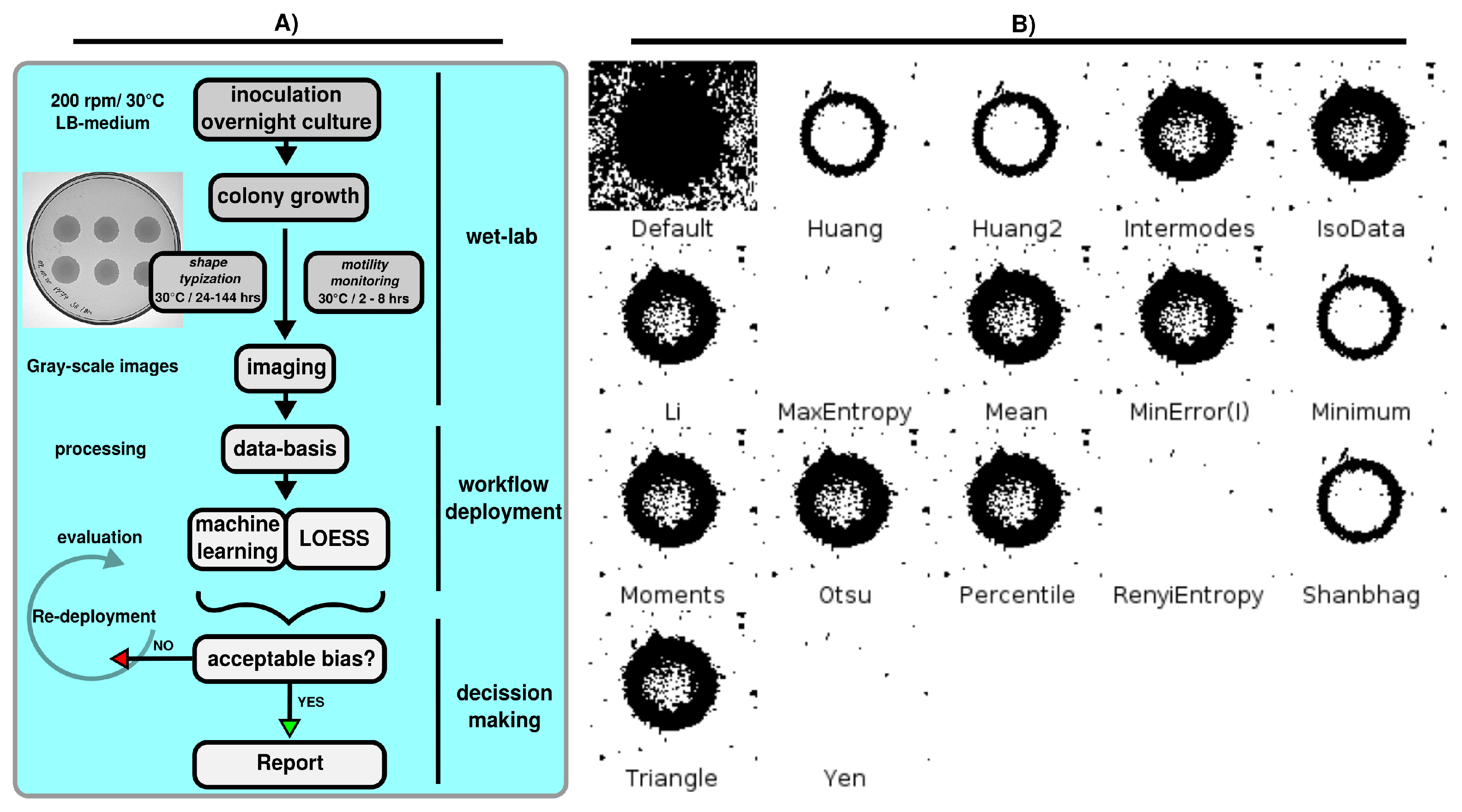
2.3.1. Image Processing

Images are deposited within a raw database from which all processing and further analysis steps are relocated to. Initially, images are re-scaled from inches to cm and transformed into binary representations. Each colony is cropped individually from whole raw images of variable sizes. Gray-scale images are automatically processed and converted to binary using a custom ImageJ2/FIJI [29,30,31,32] pipeline. Kuwahara filtering is applied for noise reduction and images are thresholded using the ‘Otsu’ algorithm (see Figure 1) [34] for all phenotypes except W3610 which is thresholded using ‘Percentile’ algorithm [35]. Individually processed colonies that are imaged at least three times for each LB agar plate are all pooled into a database for each phenotype.

2.3.2. Principal Component Analysis (PCA)

PCA is used to decompose the image data into dimensionality-reduced information that can be further used to identify clusters that are representatives for distinct colony formation states [36,37]. PCA can help to reduce the amount of irrelevant information (unspecific noise for instance) whilst maintaining characteristic clusters that are representative for respective conditional states. PCA can be usefully applied prior to further machine learning problems, primarily clustering, in order to reduce the amount of information. Contours of binary images are extracted and measured using the celltool software as described in [14] (available at https://github.com/zpincus/celltool (accessed on 15 September 2022)). Results are stored to a .csv-file and exported to an R-workflow [22,28] for plotting and cluster evaluation (see Section 2.3).

2.3.3. Density-Based Spatial Clustering Applications with Noise (DBSCAN)

DBSCAN is an unsupervised machine learning technique that aims to extract cluster information from data. For broad ML tasks that are focused on anomaly detection within the provided data, dimensionality reduction using PCA-based decomposition can be used to improve the ability of the DBSCAN algorithm to detect structure in data more performative and correctly [38,39,40]. In contrast to other clustering methods, DBSCAN allows noise between the clustered objects and is therefore considered as being more robust in discriminating different clusters more precisely [41]. In this study, DBSCAN is established using the R-packages dbscan [42], fpc [43] and further convenience packages [33,44,45,46]. Probably the most important aspect for appropriate application of DBSCAN is the parameter adjustment for minPts and $ϵ$-value. $ϵ$ should be as small as possible [47]. To access this information, k-nearest-neighbor (k-NN) [48,49] distance plots can be used to find the optimal value. A critical point in this approach is to choose an appropriate number of k-clusters for distance measurements. A useful approach involves the ‘elbow-method’ that limits k-NN along the total within sum of squares. Subsequently, the optimal $ϵ$-value can be approximated from plotting the k-NN distance against the number of data points sorted by distance. However, besides technical parameter-tuning options, the ability of the data scientist who conducts the work is important to judge if the clusters are making sense [47]. For instance, it is a good option to involve appropriate controls such as noise, for instance, that can be clearly identified as not relevant. Along this logical assumption, clusters can be adjusted and ideally optimized using basic ground truth based on a priori knowledge. In our study, we evaluate the optimal configuration of DBSCAN according to a combination of the above-mentioned aspects, referring to the recommendation statement made by Sander et al. [50] for initial k-NN distance search:

$$\begin{array}{c}\hfill minPts=2\times dim\end{array}$$

where minPts = minimal points density, dim = problem dimensionality.

3. Results and Discussion

3.1. Commonly Used B. subtilis Strains Show Distinct Colony Shape Phenotypes

B. subtilis propagates as distinct and strain-specific colony phenotypes when grown on solid media over several days (see Figure 2, Figure 5 and Figure 6). As pointed out in Figure 2B,C,E,F, the zones of different densities can be differentiated based on gray-scale images (see Figure 6). W3610 is by far the strain with the highest variation in shape types, as shown in Figure 5. Strain 168 shows two shape types followed by the least heterogeneously shaped PY79 and BG214 contour populations. The wild-type isolate W3610 is known to secrete a complex matrix containing, among other compounds, exopolysaccharides; surfactants, such as the lipo-peptide surfactin; or proteins, such as the polymer-forming TasA. This matrix expands in an arbitrarily shaped forecourt around the colony. Non-biofilm-building lab strains, such as BG214, on the other hand, form a more compact colony from which small cellular rafts originate. By choosing an appropriate threshold method, the expanding edge of these colonies can be detected and followed over time. Corresponding to that, the flagella-based motility of B. subtilis on soft-agar plates can be documented. As shown in Figure 4A, the flagellated phenotypes show a faster growing area on plates over time. Furthermore, the ability to swarm using surfactin-coated surfaces to modulate hydrophobic interactions is shown by the exponential colony growth of W3610. Strain 168 grows faster than PY79 and BG214 and shows an increased heterogeneity of the colony areas over time (see Figure 4B). Here, 168 cells conquer the surrounding media faster than its relatives PY79 and BG214 but slower than the wild-type strain W3610. Our workflow can quantify these differences as the area growth over time and approximates the motility between single measurements by using locally estimated regression curves. These strains can also be differentiated based on a PCA of different swarming behaviors, especially when comparing the flagella-deficient strain PY79yhbEF with W3610. Exchanging the genes yhbE and yhbF by a resistance cassette in the strain PY79 was described to abolish the flagella hock and filament formation in this strain [11]. Therefore, we utilized this strain as a negative control, and the colony area extension here results from an increase in the cell density and does not rely on active flagella movement. As shown prior to this study, the effect of a bactofilin double mutant on motility is present in PY79, but not in 168 or W3610, indicating strain-specific differences in the regulation of flagella biosynthesis as described in [4].

3.2. Strain-Specific Colony Formation Growth Patterns Contain Characteristic Colony Formation Shapes

The results obtained from the conducted workflow show the distinct formation of cell colonies that illustrate the variation which is possibly connected to the phenotypic expression of distinct growth behavior. Crone formations at the edge of the biofilm can be explained by the presence of flagellating cells, resulting in more diffusive areas indicating swarming. The phenotypes that do not divide into isolated cells nor swarm show less formation of this characteristic pattern. Although the availability of nutrition is more or less equally distributed in the agar plates, the results could also support a nutrition-gradient-directed growth explanation and a selective advantage for cells that can more easily conquer novel areas and build more resistant structures, such as a colony or a biofilm [51]. The applied machine learning workflow proved to be a useful monitoring tool for this purpose if applied to a relatively small but heterogeneous dataset. However, the scope of the work is to provide a useful workflow to address more detailed and informative biological questions in a systematic manner. The efficient and precise monitoring of cell viability is the key for every successful biotechnological assay formulation. By applying the presented workflow, important generalization and feature discovery aspects are addressed: First, although the same species is monitored, clearly distinct patterns of dynamic colony growth are detectable between strains (see Figure 4). Second, using a set of different time scales allows to produce a pooled but representative dataset regarding the overall shape heterogeneity and variances along the phenotypic distribution patterns (see Figure 5 and Figure 6). Interestingly, there is a hierarchical difference between the typization and motility if focusing on BG214 and PY79. BG214 resembles the flagella knock out more in terms of reduced motility, even compared to the PY79 wt (see Figure 4). However, in regards to conquering new media, BG214 shows more shape heterogeneity than PY79 (see Figure 6). A time series (1 hour (h) intervals) of B. subtilis (BG214) shows an increasing cellular area resulting from the colony density rather than motility (see Figure 2 and Figure 4). In this study, we know which strains are different regarding their growth behavior through the extensively studied model-organism B. subtilis (see Table 1) which provides a certain ground truth.

3.3. Phenotypes Can Be Discriminated According to Their Swarming Behavior

B. subtilis lab strains exhibit different swarming behaviors which can be monitored on soft-agar plates (see Figure 3). The PCA of the shape/area data shows a clear and simple representation over the dataset (see Figure 3 and Figure 4). The increased variance resulting from the angled contour shape of the W3610 8h samples can easily be recognized by the broader point distribution in the PCA plot. In contrast to this, the colonies of the non-motile strain PY79 yhbEF, as illustrated in purple, only cluster within a very small area due to their low change in variance over the course of this experiment. The colonies of its motile counterpart PY79 wt, here illustrated in blue, start to spread over the surface of the soft agar over time, resulting in bigger variances. According to that, the colonies of 168 cluster in the larger area as compared to PY79 wt. Figure 4A summarizes the motility of all five strains. Similar to Figure 3B, the originally isolated strain W3610 (olive-green) is highly motile, covering on average 500 mm${}^2$ of the plate per colony after 8h of incubation. The model also points out the smaller differences between the strains, as shown in Figure 4B. The 168 colonies (red) cover the soft agar faster than the PY79 colonies (blue). BG214 (green) behaves similar to the non-motile strain PY79 yhbEF and only develops a positive tendency between 6 and 8 h of incubation. BG214, also known as YB886 [52], is an SP$\beta$ prophage-cured derivate of 168. Besides that, the single cells of BG214 stick together after division, forming dimers which could explain the long time lag until the colony diameters increase. A slight increase in the non-flagellated PY79 yhbEF colonies derives from an increasing cell density within the colonies. The LOESS represents a non-parametric regression technique which can flexibly be applied to visually assess the relationship between two variables, in this case, the colony area and time, making it suitable for studying a wide range of phenomena. In this case, we estimate the colony size between measurements. Because we know this process to gradually proceed, the model enables us to estimate this growth behavior even with a relatively small sample size without constant monitoring of the specimen.

3.4. Spatial Clustering Is Capable of Detecting Anomalous Colony Formation

The PCA-DBSCAN results provide proof of principle for the workflow. According to the celltool PCA analysis, the orthogonal decomposition of the investigated phenotypes results in clearly distinct but also overlapping residues (see Figure 5 and Figure 7A). Phenotypes can be discriminated as distinct clusters, as shown in Figure 7. The workflow is powerful enough to discriminate noise from a core cluster which covers all the phenotypes analyzed in the study (shown in Figure 7B). This core cluster shows a population that is not clearly distinguishable by clustering. The temporal dependencies are indicated by a gradual decreasing transparency of the objects which shows that early stage colonies cluster in the first quadrant of the PCA coordinate system. In contrast to that, the colonies cluster around the center at a later stage (see Figure 5, compare to Figure 7A,C). The domesticated strains converge to a core cluster that shows less differences regarding the shape of the colonies after adjusting a k-nearest-neighbor distance using the ‘knee-of-the-curve’ k-NN distance method (see Figure 7C). We know that the artifact cluster in Figure 7B (green) consists of objects that are definitely not defined as a region of interest (compare Figure 5). On the other hand, two distinct swarmer clusters can be detected for W3610 in Figure 7B, I (blue) and II (purple). Due to the strong shape variation of the colony formations, it is difficult to capture one unifying cluster for W3610. However, this observation confirms the idea that domesticated lab strains have a stronger resemblance to each other if compared to the wild type. The core cluster, as shown in Figure 7B (red), covers all strains along the gradual increase in the colony size over time. Interestingly, the W3610 objects are the main source of the noise objects, as shown in Figure 7B (black), which is possibly a result of the objects that could not be connected to a bigger colony object at the edges or is just image noise. As shown in Figure 5, Figure 6 and Figure 7A,B, W3610 shows the highest shape variation and general heterogeneity of variances. Analogously, this is also shown using temporal resolutions scaled to hours in Figure 3 and Figure 4.

4. Outlook

Due to the modular nature of the workflow, it is easy to also implement other algorithms if needed and to combine them accordingly. It is important to notice that the entire procedure, starting from the wet-lab work prior to the computational methods performed further downstream (see Figure 1), is an integral part of the workflow. Depending on the necessary bias-correction measures, the changes in the workflow logic can be accessed at every key stage (see Figure 1). It could be shown that the remarkable differences between the B. subtilis strains can be modeled on the basis of different evaluation strategies. Furthermore, the whole procedure is based on the freely available software and basic hardware requirements necessary for this kind of computation. Therefore, it would be plausible to extend the project toward a clinical perspective using a standardized scale-up in order to study and monitor locally traced biofilm-producing bacteria that occur in a clinical environment, for instance. Changes in the phenotype-specific growth behavior can be identified and monitored and anomalies can be detected prior to further sequencing, for instance. Screening strategies could also involve detergents and antibiotics to study the respective response in the growth behavior. In theory, the effects of the possible decontamination efficiency for improved biofilm elimination could be monitored. The high flexibility of the workflow is also interesting for applications that are conducted in locations of limited computational resources, e.g., in remote areas. By observing the response toward an antibiotic or detergent for a microorganism, minimal dosages and concentrations could be defined using the workflow. However, how reproducible the outcome is, if the same strains from other laboratories show the same behavior, needs to be validated. Nevertheless, the workflow shows how to approach these tasks systematically and dissect information, respectively. Different types of assay strategies that involve antibiotics are also possible in combination with colony formation that is monitored using time-resolved gray-scale imaging, as shown prior to this workflow [53]. Our results suggest that distinct characteristic features based on the ability to invade the surroundings are suitable to apply spatial clustering based on the DBSCAN (see Figure 7). The applied local regression model in this workflow can be easily transferred to research tasks that focus on other time-related phenomena.

5. Conclusions

B. subtilis has been a workhorse for many molecular-biological laboratories for ages. As their wild relatives in nature, domesticated laboratory strains also tend to evolve over time; therefore, it is important to control if strains from different collections are still similar enough to draw general conclusions from studying them. The phenotype-based top–down approach, as presented here, can serve as a tool for comparing these strains from different sources. We have used B. subtilis in this study as a proxy for pathogenic bacteria, such as Streptococcus pneumoniae, Staphylococcus aureus or Mycobacterium tuberculosis, where the colony morphology can distinguish between the strains of different pathogenicity. The workflow is potentially capable of detecting differences that are not necessarily easily accessible within the genome sequence and can therefore be seen as complementing time- and cost-intensive genome sequencing efforts. Besides the colony growth rate, our workflow could also be applied to describe other bacterial features, such as biofilm formation. Biofilms are a key component for understanding the persistence dynamics of associated pathogens in their ability to conquer a new area to form more persistent layers or biofilms. To uncover the basic mechanisms that govern the multi-cellular interaction networks is still enigmatic and requires appropriate validation strategies. It is therefore crucial to combine multiple analytical approaches on top of high-dimensional datasets involving temporal and spatial aspects. However, any small camera device (e.g., in a smartphone) is capable of acquiring images of sufficiently enough quality to produce useful insights into the colony formation variation of distinct B. subtilis phenotypes.

Depending on the type of research other groups are working on, key principles can be adapted and modified from this workflow in a streamline. It is therefore shown how to transparently process the data and transfer the information into a machine learning pipeline to learn about the general rules of the data. Further biological questions can be assayed with this setup at low cost. B. subtilis is one of the major model organisms to study pathogenic microbes with similar growth behavior. Furthermore, our workflow is a very useful resource to optimize the parameter setting of the DBSCAN-based clustering. Our dataset contains sufficient ground truth, which is shown by the very important observation that artifacts can be clearly detected and isolated. The same accounts for swarmer colonies that help to identify strains that are potentially more pathogenic in a sense that they predominantly assemble in persistent structures or contaminate the surrounding environment faster.

To sum up, we conclude that presenting this workflow is a potentially useful resource for research groups that try to establish a reproducible pipeline to assay their own strains for similar research tasks. They may profit from the programming workflow and easy accessibility for similar tasks, empowered by the open-source technology.

References

1. Steenken, W.; Oatway, W., Jr.; Petroff, S. Dissociation and pathogenicity of the R and S variants of the human tubercle bacillus (H37). J. Exp. Med. 1934, 60, 515. [Google Scholar] [CrossRef]
2. Smithburn, K.C. The colony morphology of tubercle bacilli: I. The Presence of Smooth Colonies in Strains Recently Isolated from Sources Other than Sputum. J. Exp. Med. 1935, 61, 395. [Google Scholar] [CrossRef]
3. Chantratita, N.; Wuthiekanun, V.; Boonbumrung, K.; Tiyawisutsri, R.; Vesaratchavest, M.; Limmathurotsakul, D.; Chierakul, W.; Wongratanacheewin, S.; Pukritiyakamee, S.; White, N.J.; et al. Biological relevance of colony morphology and phenotypic switching by Burkholderia pseudomallei. J. Bacteriol. 2007, 189, 807–817. [Google Scholar] [CrossRef] [Green Version]
4. Holtrup, S.; Graumann, P.L. Strain-dependent motility defects and suppression by a flhO mutation for B. subtilis bactofilins. BMC Res. Notes 2022, 15, 1–7. [Google Scholar] [CrossRef]
5. Patrick, J.E.; Kearns, D.B. Swarming motility and the control of master regulators of flagellar biosynthesis. Mol. Microbiol. 2012, 83, 14–23. [Google Scholar] [CrossRef] [Green Version]
6. Guttenplan, S.B.; Kearns, D.B. Regulation of flagellar motility during biofilm formation. FEMS Microbiol. Rev. 2013, 37, 849–871. [Google Scholar] [CrossRef] [Green Version]
7. Kearns, D.B.; Losick, R. Swarming motility in undomesticated Bacillus subtilis. Mol. Microbiol. 2003, 49, 581–590. [Google Scholar] [CrossRef]
8. Adler, J. Chemotaxis in bacteria. Science 1966, 153, 708–716. [Google Scholar] [CrossRef]
9. Conn, H.J. The identity of Bacillus subtilis. J. Infect. Dis. 1930, 46, 341–350. [Google Scholar] [CrossRef]
10. Youngman, P.; Perkins, J.B.; Losick, R. Construction of a cloning site near one end of Tn917 into which foreign DNA may be inserted without affecting transposition in Bacillus subtilis or expression of the transposon-borne erm gene. Plasmid 1984, 12, 1–9. [Google Scholar] [CrossRef]
11. El Andari, J.; Altegoer, F.; Bange, G.; Graumann, P.L. Bacillus subtilis bactofilins are essential for flagellar hook-and filament assembly and dynamically localize into structures of less than 100 nm diameter underneath the cell membrane. PLoS ONE 2015, 10, e0141546. [Google Scholar] [CrossRef] [Green Version]
12. Burkholder, P.R.; Giles, N.H., Jr. Induced biochemical mutations in Bacillus subtilis. Am. J. Bot. 1947, 34, 345–348. [Google Scholar] [CrossRef]
13. Spizizen, J. Transformation of biochemically deficient strains of Bacillus subtilis by deoxyribonucleate. Proc. Natl. Acad. Sci. USA 1958, 44, 1072–1078. [Google Scholar] [CrossRef] [Green Version]
14. Pincus, Z.; Theriot, J. Comparison of quantitative methods for cell-shape analysis. J. Microsc. 2007, 227, 140–156. [Google Scholar] [CrossRef]
15. Cohn, F.J. Ueber Bacterien, die Kleinsten Lebenden Wesen; CG Lüderitz: Berlin, Germany, 1872; Volume 165. [Google Scholar]
16. Julkowska, D.; Obuchowski, M.; Holland, I.B.; Séror, S.J. Comparative Analysis of the Development of Swarming Communities of Bacillus subtilis 168 and a Natural Wild Type: Critical Effects of Surfactin and the Composition of the Medium. J. Bacteriol. 2005, 187, 65–76. [Google Scholar] [CrossRef] [Green Version]
17. Bertani, G. Studies on lysogenesis I: The mode of phage liberation by lysogenic Escherichia coli. J. Bacteriol. 1951, 62, 293–300. [Google Scholar] [CrossRef] [Green Version]
18. Cleveland, W.S. Robust locally weighted regression and smoothing scatterplots. J. Am. Stat. Assoc. 1979, 74, 829–836. [Google Scholar] [CrossRef]
19. Cleveland, W.S. LOWESS: A program for smoothing scatterplots by robust locally weighted regression. Am. Stat. 1981, 35, 54. [Google Scholar] [CrossRef]
20. Cleveland, W.S.; Devlin, S.J. Locally weighted regression: An approach to regression analysis by local fitting. J. Am. Stat. Assoc. 1988, 83, 596–610. [Google Scholar] [CrossRef]
21. Wickham, H. ggplot2: Elegant Graphics for Data Analysis; Springer: New York, NY, USA, 2016. [Google Scholar]
22. R Core Team. R: A Language and Environment for Statistical Computing; R Foundation for Statistical Computing: Vienna, Austria, 2019; Available online: https://www.r-project.org (accessed on 15 September 2022).
23. RStudio Team. RStudio: Integrated Development Environment for R; RStudio, PBC., Inc.: Boston, MA, USA, 2022; Available online: http://www.rstudio.com (accessed on 15 September 2022).
24. Van Rossum, G.; Drake, F.L., Jr. Python Reference Manual; Department of Computer Science [CS]. Centrum voor Wiskunde en Informatica Amsterdam, The Netherlands (CWI). Available online: https://www.python.org/downloads/ (accessed on 15 September 2022).
25. Xie, Y. knitr: A General-Purpose Package for Dynamic Report Generation in R. R Package Version 1.39. 2022. Available online: https://rdrr.io/cran/knitr/ (accessed on 15 September 2022).
26. Xie, Y. Dynamic Documents with R and Knitr, 2nd ed.; Chapman and Hall/CRC: Boca Raton, FL, USA, 2015; ISBN 978-1498716963. [Google Scholar]
27. Xie, Y. Knitr: A Comprehensive Tool for Reproducible Research in R. In Implementing Reproducible Computational Research; Stodden, V., Leisch, F., Peng, R.D., Eds.; Chapman and Hall/CRC: Boca Raton, FL, USA, 2014; ISBN 978-1466561595. [Google Scholar]
28. Allaire, J.; Horner, J.; Xie, Y.; Marti, V.; Porte, N. Markdown: Render Markdown with the C Library ’Sundown’. R Package Version 1.1. 2019. Available online: https://CRAN.R-project.org/package=markdown (accessed on 15 September 2022).
29. Schindelin, J.; Arganda-Carreras, I.; Frise, E.; Kaynig, V.; Longair, M.; Pietzsch, T.; Preibisch, S.; Rueden, C.; Saalfeld, S.; Schmid, B.; et al. Fiji: An open-source platform for biological-image analysis. Nat. Methods 2012, 9, 676–682. [Google Scholar] [CrossRef]
30. Schindelin, J.; Rueden, C.T.; Hiner, M.C.; Eliceiri, K.W. The ImageJ ecosystem: An open platform for biomedical image analysis. Mol. Reprod. Dev. 2015, 82, 518–529. [Google Scholar] [CrossRef] [Green Version]
31. Schneider, C.A.; Rasband, W.S.; Eliceiri, K.W. NIH Image to ImageJ: 25 years of image analysis. Nat. Methods 2012, 9, 671–675. [Google Scholar] [CrossRef]
32. Rueden, C.T.; Schindelin, J.; Hiner, M.C.; DeZonia, B.E.; Walter, A.E.; Arena, E.T.; Eliceiri, K.W. ImageJ2: ImageJ for the next generation of scientific image data. BMC Bioinform. 2017, 18, 529. [Google Scholar] [CrossRef] [Green Version]
33. Wickham, H.; François, R.; Henry, L.; Müller, K. dplyr: A Grammar of Data Manipulation. R Package Version 1.0.10. 2022. Available online: https://CRAN.R-project.org/package=dplyr (accessed on 15 September 2022).
34. Otsu, N. A threshold selection method from gray level histograms. IEEE Trans. Syst. Man Cybern. 1979, 9, 62–66. [Google Scholar] [CrossRef] [Green Version]
35. Doyle, W. Operations Useful for Similarity-Invariant Pattern Recognition. J. ACM 1962, 9, 259–267. [Google Scholar] [CrossRef]
36. Pearson, K. LIII. On lines and planes of closest fit to systems of points in space. Lond. Edinb. Dublin Philos. Mag. J. Sci. 1901, 2, 559–572. [Google Scholar] [CrossRef] [Green Version]
37. Hotelling, H. Analysis of a complex of statistical variables into principal components. J. Educ. Psychol. 1933, 24, 417. [Google Scholar] [CrossRef]
38. Savvas, I.; Chernov, A.; Butakova, M.; Chaikalis, C. Increasing the quality and performance of n-dimensional point anomaly detection in traffic using pca and dbscan. In Proceedings of the 2018 26th Telecommunications Forum (TELFOR), Belgrade, Serbia, 20–21 November 2018; pp. 1–4. [Google Scholar]
39. Ni, L.; Jinhang, S. The analysis and research of clustering algorithm based on PCA. In Proceedings of the 2017 13th IEEE International Conference on Electronic Measurement & Instruments (ICEMI), Yangzhou, China, 20–22 October 2017; pp. 361–365. [Google Scholar]
40. Badrinath Krishna, V.; Weaver, G.A.; Sanders, W.H. PCA-based method for detecting integrity attacks on advanced metering infrastructure. In Proceedings of the International Conference on Quantitative Evaluation of Systems, Madrid, Spain, 1–3 September 2015; Springer: Berlin/Heidelberg, Germany, 2015; pp. 70–85. [Google Scholar]
41. Ester, M.; Kriegel, H.P.; Sander, J.; Xu, X. A density-based algorithm for discovering clusters in large spatial databases with noise. In Proceedings of the Kdd, Portland, OR, USA, 2–4 August 1996; Volume 96, pp. 226–231. [Google Scholar]
42. Hahsler, M.; Piekenbrock, M.; Doran, D. dbscan: Fast Density-Based Clustering with R. J. Stat. Softw. 2019, 91, 1–30. [Google Scholar] [CrossRef] [Green Version]
43. Hennig, C. fpc: Flexible Procedures for Clustering. R Package Version 2.2-5. 2020. Available online: https://CRAN.R-project.org/package=fpc (accessed on 15 September 2022).
44. Dowle, M.; Srinivasan, A. data.table: Extension of ‘data.frame’. R Package Version 1.14.2. 2021. Available online: https://CRAN.R-project.org/package=data.table (accessed on 15 September 2022).
45. Maechler, M.; Rousseeuw, P.; Struyf, A.; Hubert, M.; Hornik, K. Cluster: Cluster Analysis Basics and Extensions. R Package Version 2.1.1. Available online: https://CRAN.R-project.org/package=cluster (accessed on 15 September 2022).
46. Wickham, H. Stringr: Simple, Consistent Wrappers for Common String Operations. R package Version 1.4.1. 2022. Available online: https://CRAN.R-project.org/package=stringr (accessed on 15 September 2022).
47. Schubert, E.; Sander, J.; Ester, M.; Kriegel, H.P.; Xu, X. DBSCAN revisited, revisited: Why and how you should (still) use DBSCAN. ACM Trans. Database Syst. (TODS) 2017, 42, 1–21. [Google Scholar] [CrossRef]
48. Fix, E.; Hodges, J.L., Jr. Discriminatory Analysis-Nonparametric Discrimination: Small Sample Performance; Technical Report; California Univ Berkeley: Berkeley, CA, USA, 1952. [Google Scholar]
49. Cover, T.; Hart, P. Nearest neighbor pattern classification. IEEE Trans. Inf. Theory 1967, 13, 21–27. [Google Scholar] [CrossRef]
50. Sander, J.; Ester, M.; Kriegel, H.P.; Xu, X. Density-based clustering in spatial databases: The algorithm gdbscan and its applications. Data Min. Knowl. Discov. 1998, 2, 169–194. [Google Scholar] [CrossRef]
51. Matsushita, M.; Fujikawa, H. Diffusion-limited growth in bacterial colony formation. Phys. A Stat. Mech. Its Appl. 1990, 168, 498–506. [Google Scholar] [CrossRef]
52. Yasbin, R.E.; Fields, P.I.; Andersen, B.J. Properties of Bacillus subtilis 168 derivatives freed of their natural prophages. Gene 1980, 12, 155–159. [Google Scholar] [CrossRef]
53. Mayer, B.; Schwan, M.; Thormann, K.M.; Graumann, P.L. Antibiotic Drug screening and Image Characterization Toolbox (ADICT): A robust imaging workflow to monitor antibiotic stress response in bacterial cells in vivo. F1000Research 2021, 10, 277. [Google Scholar] [CrossRef]
Figure 1. (A) Schematic illustration of the presented workflow showing key stages of the pipeline. Improvements can be established using densely conducted documentation in combination with useful information that resulted after re-deployment during bias-minimization steps. These can start at every stage of the pipeline. However, maintaining the database is of key importance due to the fact that downstream processing and analysis is directly influenced upon changes that are made to the data. Data management is indispensable for reproducible research using machine learning. Therefore, a modular set of pipeline and workflow segments are the best choice due to enhanced accessibility. (B) Montage shows listed thresholding algorithms applied to a B. subtilis colony. Depending on a representative inclusion/exclusion of pixel values involved in the thresholding, binary image processing can be conducted dynamically using an automated IJ processing script. Resulting binary images are further processed and analyzed to quantify occurrences of phenotype-specific differences along the shape and curvature of respective colonies using unsupervised learning based on celltool [14]. Illustration created using Inkscape 0.92.3, available at: https://www.inkscape.org (accessed on 15 September 2022).
Biomedinformatics 02 00036 g001
Figure 2. Characteristic B. subtilis colony differences. (A) BG214 shows characteristic cones located at the edges of the colony. (B) The overall absorption is remarkably stronger for the total colony area. Areas outside of the densely packed colony are clearly distinct because light can pass through easier there. Whilst BG214 forms restricted colony of more or less homogenous biomass density, W3610 shows gradients of biomass density represented by more light passing through the observed area. (C) Topographic representation of the colorimetric representation of the colony shows a plateau-like distribution of absorption maximum located throughout the whole colony. (D) In contrast to (A), W3610 shows different absorption densities, illustrating the strong ability of the phenotype to swarm. (E) Areas where cells are not densely packed allow more light to pass. (F) Inverted representation of W3610 shows unidirectional increase in waveform indicated by increased absorption. Furthermore, the center of the colony is not a plateau but indicates a ring shape separating the interior. It can be concluded that the wild-type W3610 phenotype is more agile regarding its invasiveness toward the surrounding medium. Figure created using Inkscape 0.92.3, available at: https://www.inkscape.org (accessed on 15 September 2022) and ImageJ2/FIJI 2.7.0/1.53t, (available at: https://fiji.sc/ (accessed on 15 September 2022)). False-colored in ‘ICA3’. Scale bars = 1 cm.
Biomedinformatics 02 00036 g002
Figure 3. (A) Processing of an overgrown soft-agar plate. B. subtilis W3610 rapidly spreads over the surface of soft-agar plates and single colony borders are not distinguishable after 8 h. To approximate the area, the plate was sectioned, and threshold was adjusted manually. (B) Colony data plotted based on the shape variance (normalized model 1 and 2) of their contours that are extracted and measured from binary images using celltool [14]. The distribution of colony contour shape gives additional information on the motility and shape differences between B. subtilis strains PY79 (blue), 168 (red), BG214 (green), W3610 (olive-green) and the flagella-deficient strain PY79 yhbEF on soft-agar plates. Colony area is indicated by the size of the spots in the plot and time of detection is indicated by the transparency, with the most transparent spots being acquired at 0 h and the most dense spots being acquired at 8h. Figure created using Inkscape 0.92.3, available at: https://www.inkscape.org (accessed on 15 September 2022) and the R-package ggplot2 [21] available at: https://ggplot2.tidyverse.org (accessed on 15 September 2022).
Biomedinformatics 02 00036 g003
Figure 4. Motility of B. subtilis strains assayed on soft-agar plates illustrated as smoothed scatter plot of colony area plotted against incubation time. Conditional means were smoothed using LOESS regression with the 95% confidence intervals illustrated in gray. (A) Strains PY79 (blue), 168 (red), PY79 (turquoise), BG214 (green), W3610 (olive-green) and the flagella-deficient PY79 derivate PY79 yhbEF (purple) are compared, conditional means were smoothed using LOESS regression. (B) Separate comparison of 168 wt, PY79 wt, BG214 and PY79 yhbEF. Figure created using Inkscape 0.92.3, available at: https://www.inkscape.org (accessed on 15 September 2022) and the R-package ggplot2 [21] available at: https://ggplot2.tidyverse.org (accessed on 15 September 2022).
Biomedinformatics 02 00036 g004
Figure 5. Distribution of shape contours including noise (smaller cell assemblies and artifacts) shows that distinct curvatures can be identified along the distinct phenotypes. W3610 (blue) shows the most heterogeneous and strong curved shape followed by 168 (orange). Both swarmer phenotypes are clearly distinct compared to the less motile strains PY79 (green) and BG214 (magenta). Remarkably, W3610 localizations are less centered compared to the other strains, especially PY79, which indicates the ability to swarm and conquer the surrounding media faster and can be relocated to specific localization patterns as shown here using principal components based on the area and curvature. Keeping in mind that the dataset consists of a repeatedly acquired and temporarily pooled set of gray-scale images, it is powerful enough to monitor the underlying heterogeneity of variances between the isolated contours of the respective phenotypes. Figure created using Inkscape 0.92.3, available at: https://www.inkscape.org (accessed on 15 September 2022) and celltool [14].
Biomedinformatics 02 00036 g005
Figure 6. PCA results (after noise elimination of results shown in Figure 5) show distinct colony shape types. Isolated and iterated colony shapes are compared between the monitored phenotypes. Corresponding to Figure 5, colony shapes can be distinguished along their shape variance which tends to be remarkably higher for W3610 and 168 compared to BG214 and PY79, supporting the idea that this could be connected to the aspect of domestication and the ability to swarm. Figure created using Inkscape 0.92.3, available at: https://www.inkscape.org (accessed on 15 September 2022) and celltool [14].
Biomedinformatics 02 00036 g006
Figure 7. PCA-DBSCAN analysis of B. subtilis. (A) Principal components of PY79 (purple), 168 (red), BG214 (blue) and W3610 (olive-green) colony contours are plotted in a scatter plot. Time of colony growth is indicated by spot transparency. (B) Cluster anomaly detection and discrimination of principal components. DBSCAN identified three clusters, the core colony shapes (red), the arbitrary-shaped swarmer colonies (blue and purple) and artifacts from contour detection (green). The epsilon value was adjusted according to the distances of the 4 nearest neighbors as illustrated on the right. (C) Separate clustering of single strains. ϵ -values were adjusted manually according to the 4 nearest-neighbor distances shown below. Identified clusters are depicted for strains PY79, BG214, W3610 and 168. Figure created using Inkscape 0.92.3, available at: https://www.inkscape.org (accessed on 15 September 2022) and ggplot2 [21] available at: https://ggplot2.tidyverse.org (accessed on 15 September 2022).
Biomedinformatics 02 00036 g007