Abstract
Behavioral factors can affect the blood glucose (BG) levels in people with type 1 diabetes (T1D), therefore, their effects need to be incorporated in blood glucose management for these individuals. Accordingly, in this work, we study the effect of two behavioral states, physical activity (PA) and stress state (SS), on BG fluctuations in individuals with T1D. We provide two methods for quantifying biomarkers related to PA and SS using raw acceleration (ACC) and electrodermal activity (EDA) data collected with a wearable device. We evaluate the impact of PA and SS on BG fluctuation by adding the derived behavior-related biomarkers in two cutting-edge deep learning-based glucose predictive models, a long short-term memory (LSTM) and a convolutional neural network (CNN)-LSTM network, for prediction horizons (PHs) of 30, 60 and 90 min. Through an ablation study, we demonstrate that incorporating the estimated behavior-related biomarkers improves the BG predictive model’s performance obtaining mean absolute error (MAE) 9.13 ± 0.95, 17.75 ± 1.93 and 31.85 ± 2.88 in [mg/dL], root mean square error (RMSE), 12.35 ± 1.06, 24.71 ± 2.31 and 41.64 ± 4.12 in [mg/dL], and coefficient of determination (R2), 95.34 ± 3.34, 78.87 ± 4.35 and 60.11 ± 4.76 in [%], for the LSTM model; and MAE 9.37 ± 0.88, 17.87 ± 1.67 and 29.47 ± 2.13 in [mg/dL], RMSE 12.51 ± 1.40, 24.37 ± 2.49 and 39.52 ± 3.89 in [mg/dL], and R2 94.65 ± 3.90, 78.37 ± 4.11 and 61.12 ± 4.30 in [%], for the CNN-LSTM model, respectively, across all PHs. Additionally, we illustrate the generalizability of the proposed models by performing both population- and patient-wise.
1. Introduction
Despite significant efforts devoted to the problem of blood glucose (BG) prediction in people with Type 1 Diabetes (T1D) over the last several decades [1,2,3,4,5,6,7,8,9] challenges associated with glycemic disturbances due to daily unrepresented inputs, such as behavioral states, are largely under researched. In this regard, perhaps the most crucial challenge is that of accounting for the effect of daily physical activity (PA), both structured and unstructured, and emotional or psychological stress state (SS), in the prediction of BG, as a steppingstone toward the design of appropriate treatment decisions. To date, several studies have proposed various methodologies to investigate the impact of such glycemic disturbances on BG level fluctuations, enabled by the advent of continuous glucose monitoring (CGM) devices, and the growing use of consumer-grade wearable devices [10], which facilitated keeping track of BG levels as well as other physiological variables almost continuously and in a minimally invasive manner. Facciolli et al. [11] investigated the benefits of including steps count measured by an off-the-shelf wearable device, as a proxy for PA, together with insulin and meal information, in a linear black box model identified from actual patient data. The authors reported improved predictions accuracy when including PA in their model. Some studies included additional inputs related to physical exercise to the glucose metabolism model: Refs. [12,13] used a quantized signal representing the level of exercise in an artificial neural network, while [14,15,16] employed an estimate of energy expenditure in linear multivariate models. Bertachi et al. [17] used multilayer perceptron (MLP) and support vector machine (SVM) to predict nocturnal hypoglycemia (NH) in the daily life of T1Ds including the effect of PA, however, they reported the manual feature extraction and high computational cost as the limitations of their methodology. More recently, Sevil et al. [18] demonstrated that by incorporating new features for the type and intensity of PA and acute psychological stress (APS), generated using ML techniques, as exogenous inputs into an adaptive system identification framework, the accuracy of one-hour-ahead BG prediction improved. De Paoli et al. [19] used a specific type of ANN, Jump Neural Network, to overcome the challenges associated with the prediction of abrupt changes in BG values caused by PA. However, as a result of testing on a small number of patients, they asserted that their results cannot be considered conclusive, and their method has an additional computational load that does not justify the insufficiently significant gain achieved.
Against this background, a more comprehensive model that is generalizable to a larger group of individuals with T1D, applicable to daily life events, computationally efficient, and has a robust performance, specifically for higher prediction horizons, is needed for improved BG management.
In a previous study [9], we have obtained encouraging preliminary results pertaining to BG prediction with a hybrid CNN-LSTM model using meal information, insulin intake and CGM data on a dataset [4] comprised of 59 individuals with T1D who had participated in a three-day in-hospital study. Our investigation demonstrated that our model achieved superior glucose forecasting for up to 90 min PH, compared to existing approaches in the literature. It is of interest, therefore, to study whether we can further improve the prediction accuracy and generalize our model to a wider range of people with T1D in the outpatient setting, by accounting for glycemic disturbances occurring in daily life including PA and SS. Our aim is therefore to characterize the effect of physical activity and stress on blood glucose fluctuations by using data collected with wearable devices, and incorporate it into state-of-the-art BG predictive models to achieve more accurate BG predictions.
To this end, we propose a 2-steps approach: in the first step, we derive biomarkers for PA and SS from raw accelerometer (ACC) and electrodermal activity (EDA) signals collected by a wearable device. In the second step, we combine the obtained biomarkers with the CGM, meal and insulin intakes in a multivariate dataset and feed it to our DL-based glucose predictive model to forecast the future BG values. We validate our novel approach on a publicly available dataset of 6 T1D patients whose data were recorded during an 8-weeks trial under free-living condition [20].
The remainder of the article is organized as follows. The Materials and Methods Section contains experimental data and a description of the data pre-processing pipeline followed by description of the proposed algorithms for quantifying PA and stress levels, as well as an explanation of the proposed prediction strategy. The Results Section presents the population-wise and patient-wise results, separately, as well as a comprehensive comparison with similar studies in the literature. Finally, the Discussion and Conclusion section contains a discussion of the proposed method’s advantages and limitations, as well as the study’s conclusion.
2. Materials and Methods
2.1. Experimental Condition
The dataset used in this work was the OHIOT1DM dataset [20] comprises of eight weeks of data collected from 12 people with T1D. The data consists of periodic blood glucose measurements, information regarding administered insulin, different biometric data, and self-reported meals and exercise information which was released in 2020 for the second edition of the BG Level Prediction (BGLP) Challenge [21], a competition in which the participating researchers were expected to produce BG predictions for 30 and 60 min PH using a common dataset and evaluate the performances of their algorithms according to predefined metrics. The dataset is distributed in two separate files for the train and test sets. Each file contains data from six individuals with T1D identified anonymously as 540, 544, 552, 567, 584, and 596 who were on insulin pump therapy (Medtronic 530G and 630G [22]) and wore Medtronic Enlite [23] CGM sensors during the eight-week data collection period. The dataset includes BG concentration collected by a CGM device with a 5 min sampling rate, basal and bolus insulin doses, self-reported ingested carbohydrate (CHO) intake estimates, self-reported exercise, sleep, work, stress, and illness. Additionally, all subjects were required to wear an Empatica Embrace [24] fitness band throughout the study, which recorded one-minute aggregations of EDA, skin temperature, and magnitude of ACC.
The ACC and EDA signals presented many missing samples, as it is common in dataset collected in real-life situations. Previous studies that used this dataset omitted indeed these two signals because of this problem, and thus ignored the effect of PA and stress level on BG level prediction [25,26,27,28,29]. In our case, we used a linear interpolation algorithm to estimate the missing data samples when the gaps between samples were less than 60 min, while for gaps greater than 60 min, corresponding data were discarded.
All sensors’ data were synchronized, and the variables of interest, namely BG, ACC, and EDA, were uniformly resampled at 15 min sampling intervals. Next, each feature was normalized and standardized independently to ensure that the model was not biased toward any particular variable.
2.2. Physical Activity Intensity Estimation
In a previous work [30] we proposed to detect PA and grade its intensity with a novel threshold-based algorithm. The method exploited the magnitude of the average third-order time derivative of the 3D displacement retrieved from three-axis accelerometer data low-pass filtered at 1[Hz] to isolate the static component due to gravity. User-determined activity intensity thresholds from sedentary to vigorous activity, were tuned to patient self-reported low, moderate and high fitness conditions, using more than 5000 h of outpatient subject data available. More detailed information regarding the methodology, are provided in the paper [30].
In the current study, we apply the same methodology, with appropriate modifications accounting for the differences in the sampling frequency of the raw ACC signals, to obtain the biomarker for physical activity intensity, which we call Physical Activity Intensity (PAI) from now on.
2.3. Stress State Estimation
In this work, we focus on detecting and monitoring changes in the sympathetic arousal state triggered by the fight-or-flight response to emotional stress. EDA signal has two components: tonic component which is a slow varying signal and phasic component which incorporates the sudden neural spikes corresponding to physiological changes. It has been demonstrated that an increase in the frequency of these spikes relates to an increase in patients’ stress levels [31]. Accordingly, in [32], Wickramasuriya et al. proposed to deconvolve EDA signal to obtain neural impulses that stimulate sweat glands using a two-step optimization formulation that simultaneously recovers sparse neural stimuli and estimates physiological system parameters. Then, in a previous study [33], we proposed that sympathetic arousal states can be quantified from skin conductance measurements collected with a wrist-worn device.
For each stress event, the corresponding hidden cognitive state was defined as a function of previous cognitive states , state defining variable , external stimuli variable, and , and noise component, :
where and are obtained through assessing the stress event and modeling the increase in it at any timestamp. Therefore, the hidden state was computed for each time point through an iterative process. More detailed information and formulation can be found in [33].
Correspondingly, in this study we leverage this methodology to obtain a biomarker representing the quantified estimation of stress level obtained from raw EDA signal in the OHIOT1DM dataset. We call this feature Stress State Index (SSI) from now on.
Figure 1 shows the available data along with the proposed biomarkers for a representative subject in the study.
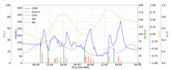
Figure 1.
Representative subject’s data: CGM [mg/dL] (blue); CHO intake [g] (green); insulin doses [u] (red); PAI [a.u.] (purple) and SSI [a.u.] (yellow) vs. Time of the day [HH:MM].
2.4. Input-Output Partitioning
We concatenated and aligned the obtained PAI and SSI with BG concentration measured by CGM, self-reported ingested CHO and insulin intakes, to create the multivariate dataset to be used for prediction. Then, a sliding window with a step size of one was rolled over the multivariate dataset to generate sequences of corresponding input, , and output, , sets for training the proposed DL-based BG prediction model depending on the user-specified PH. By construction, each windowed sample , is a retrospective snapshot of all variables corresponding to a sequence of future CGM values, , , such that:
where , stands for the window index with n the total number of input windows generated by rolling the sliding window all over the multivariate time series. , is a vector representing the jth feature with showing the number of features used for training the model. We investigate the effect of PAI and SSI on the performance of the GC predictive model via an ablation study; thus, n varies depending on the scenario. For example, when CGM, CHO, and insulin are used as inputs to the model, = 3, whereas when PAI and SSI are added to those three variables, = 5.
2.5. Glucose Predictive Model
To investigate the feasibility of our hypothesis, we build on our previously published hybrid CNN-LSTM model [9]. The input samples are historical windows of data, containing BG values, meal, and insulin intakes information, as well as PAI and SSI samples, biomarkers as described in Section 2.2 and Section 2.3, for time interval of as the input, such that for with , total number of windowed training samples, with model parameters and number of parameters. These samples are sent into the CNN component so that significant features are extracted. The produced feature vectors are then input into two LSTM layers, which learn the variables’ temporal dynamics and causal relationships. Finally, the output of the final LSTM layer is embedded into two fully connected layers, where each neuron is connected to every neuron in the preceding layer, in order to interpret the non-linear combination of these features and predicted future BG values , for up to a user specified PH, in the output layer. The proposed model architecture is depicted in Figure 2. For comparison purposes, we designed a second model comprised of two layers of LSTM network followed by three fully connected layers. The third fully connected layer is the output layer which contains predicted future BG values , for up to a user specified PH, given the input samples, structured in the same as what explained for the CNN-LSTM model. The proposed LSTM model architecture is depicted in Figure 3. It should be noted that for model architecture and hyperparameters selection, we run grid search to make sure the best possible model is designed.
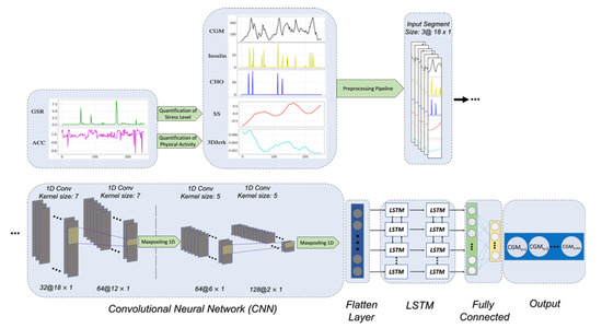
Figure 2.
The architecture of the proposed CNN-LSTM model. Raw ACC and EDA signals are used to estimate PAI and SSI features, respectively. Then, these generated features, along with the CGM, insulin, and CHO signals are passed through the preprocessing pipeline.
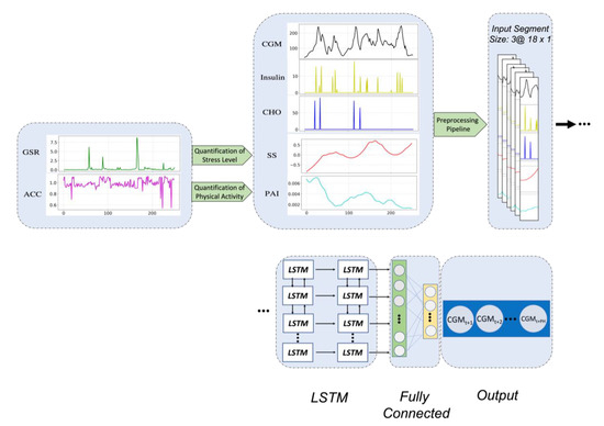
Figure 3.
The architecture of the proposed LSTM model. Raw ACC and EDA signals are used to estimate PAI and SSI features, respectively. Then, these obtained features, are combined with the CGM, insulin, and CHO timeseries and are passed through the preprocessing.
The training procedure is carried out by backpropagating the error via the network layers and changing the weights in such a way that the loss function is minimized, i.e., the model learns to predict the future BG value as close to the actual value as possible. Following each convolutional layer, a batch normalization operation is performed to re-center and scale the input features for the subsequent layer. By standardizing the parameters, this stabilizes the learning process and minimizes internal covariance shift. Additionally, in both models, a dropout layer is utilized following each LSTM layer to minimize overfitting by randomly setting certain input units to zero during training.
We used the TensorFlow framework [34] in Python 3.7 programming language to build and implement our models. The training set was divided into train and validation subsets with an 80:20 ratio, respectively. To minimize loss and optimize the cost function, the root mean square propagation (RMSProp) approach was adopted with a moving average parameter of 0.9 and an initial learning rate of 0.0001. The model was trained for 300 epochs with a batch size of 128 while an early stopping point strategy was utilized to minimize over-training by monitoring changes in validation loss with a patience of 50 epochs.
3. Results
In this section, we present results obtained on eight weeks of real-life data for six T1D patients from the OHIOT1DM 2020 dataset [20].
3.1. Evaluation Metrics
Several metrics were utilized to evaluate the proposed model’s performance and the influence of incorporating PAI and SSI in our computations: the mean absolute error (MAE), the root-mean- square error (RMSE), and coefficient of determination (R2). Equations (5)–(7) report the formulas used for their calculation, where n is the total number of windowed samples, and are the actual and predicted GC values at time and in R2 is the mean value of all samples:
Using these metrics will enable us to compare our results to those of other research studies in the literature.
3.2. Evaluation Scenarios
We evaluated our proposed models with seven distinct scenarios, summarized in Table 1. Scenario 1 represents the baseline case, containing CGM, CHO and insulin intakes, while in Scenario 2 and 3, raw EDA and ACC signals, representing the effect of SS and PA, respectively, are included into computations, to investigate the effectiveness of incorporating PA and SS in BG predictive model’s performance. In Scenario 4 and 5 the biomarkers for PAI and SSI are added to the baseline case, to be compared with scenarios 2 and 3, respectively, in terms evaluating the changes in results obtained as a result of the two quantification methodologies. Finally, Scenarios 6 and 7 incorporate the raw ACC and EDA, and PAI and SSI, respectively, to the baseline. The rationale behind defining these scenarios is to differentiate the influence that the raw EDA and ACC signals may have on BG prediction compared to that of the estimated biomarkers for SSI and PAI.

Table 1.
Scenarios considered in our ablation study to understand the contribution of different variables on BG prediction performance.
3.3. Population-Wise Analysis
We employed training sets of all patients for population-wise analysis, and then test sets of all six individuals for performance evaluation in order to forecast future BG values for an unknown data sample. The model was trained on three distinct PHs, namely 30, 60, and 90 min. Table 2 and Table 3 show the performance of the proposed LSTM and CNN-LSTM algorithms for different scenarios in terms of MAE [mg/dL], RMSE [mg/dL] and R2 [%] metrics, respectively.
Table 2.
Population results for LSTM model. RMSE [mg/dL], MAE [mg/dL] and R2 [%] for 30, 60 and 90 min ahead BG prediction, for different scenarios.
Table 3.
Population results for CNN-LSTM model. RMSE [mg/dL], MAE [mg/dL] and R2 [%] for 30, 60 and 90 min ahead BG prediction, for different scenarios.
Although adding raw EDA and ACC in Scenarios 2, 3 and 6 improved results slightly comparing to the baseline, using the computed biomarkers SSI and PAI in Scenarios 4, 5 and 7 significantly improved model performance, demonstrating the validity of our suggested methodologies for producing these two biomarkers and including them in the prediction model. Overall, the best results for both models are obtained in Scenario 7, as highlighted in bold face characters in the tables.
3.4. Patient-Wise Analysis
We evaluate the suggested models patient-by-patient, training and testing a tailored model on each patient’s data, in order to address the inter-subject variability inherent in T1D. Table 4 and Table 5 illustrate the proposed LSTM and CNN-LSTM model’s performance in terms of MAE [mg/dL], RMSE [mg/dL], and R2 [%] metrics in predicting future BG for each patient individually, respectively, using the same patient’s data as the training and test sets and Scenario 7 as the training scenario.
Table 4.
Patient-wise analysis results with LSTM model, given scenario 7. MAE, RMSE and R2 of BG prediction for personalized training for each patient separately, for 30 to 90 min PH.
Table 5.
Patient-wise analysis results with CNN-LSTM model, given scenario 7. MAE, RMSE and R2 of BG prediction for personalized training for each patient separately, for 30 to 90 min PH.
Additionally, the box plots in Figure 4 depicts the distribution of the resulting metrics for the patient-wise analysis for both models. Although the model performance degrades when compared to the population-wise analysis, the distribution of the findings across all individuals remains favorable, indicating the generalizability of the suggested methods across a diverse collection of T1D patients.
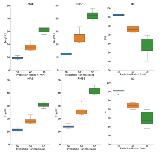
Figure 4.
Box plot showing the patient-wise results for (top) LSTM and (bottom) CNN-LSTM models in terms of (left) MAE, (middle) RMSE and (right) R2 metrics, given scenario 7 as dataset. In each panel, blue, orange and green are boxplots for 30, 60 and 90 min.
3.5. Comparison with Existing Methods
Table 6 compares our results to the top five ranked research works that participated in the 2020 BGLP challenge [21]. Studies were evaluated based on MAE [mg/dL] and RMSE [mg/dL] for 30 and 60 min PH and ranked according to the overall accuracy defined as the summation of MAE and RMSE in [mg/dL]. We see that our work outperforms the previous research across all metrics and overall performance. Contributions are identified by their Paper ID, as syndicated on the official BGLP challenge ranking page [21].
Table 6.
Comparison of our results and the top five ranked research works that participated in the 2020 BGLP challenge. Population mean ± (standard deviation) of accuracy metrics (MAE and RMSE) for 30 and 60 min ahead BG prediction.
4. Discussion and Conclusions
In this work, we analyzed whether the incorporation of our proposed biomarkers for PA and SS, computed from raw ACC and EDA signals collected with a commercially available wearable device, improved the BG prediction accuracy for PH ranging from 30 to 90 min. We compare the performances of our previously published CNN-LSTM prediction model [9] with those of a novel LSTM-based predictor. At a population level, as far as the CNN-LSTM model is concerned, our results demonstrate a decrease in RMSE of 6.84 ± 3.01 [mg/dL], 7.31 ± 2.08 [mg/dL] and 6.6 ± 6.41 [mg/dL] for 30, 60, 90 min PH, respectively; a decrease in MAE of 3.96 ± 2.08 [mg/dL], 4.45 ± 3.53 [mg/dL] and 4.73 ± 3.77 [mg/dL] for 30, 60, 90 min PH, respectively; and an increase in R2 of 3.78 ± 6.77 [%], 9.55 ± 7.38 [%] and 7 ± 7.01 [%] for 30, 60, 90 min PH, respectively, from Scenario 1 to Scenario 7. While considering the LSTM model, instead, the reduction in RMSE is 5.97 ± 2.74 [mg/dL]; 8.55 ± 2.33 [mg/dL] and 7.12 ± 6.96 [mg/dL] for 30, 60, 90 min PH, respectively; a reduction in MAE of 3.85 ± 2.21 [mg/dL], 5.23 ± 3.48 [mg/dL] and 5.26 ± 4.58 [mg/dL] for 30, 60, 90 min PH, respectively; and an increase in R2 of 3.8 ± 5.46 [%], 11.95 ± 8.10 [%] and 10.35 ± 8.41 [%], respectively, when comparing Scenario 1 with Scenario 7. These findings validate our hypothesis that adding our proposed biomarkers is indeed beneficial for improved BG prediction, especially on longer PH. When comparing the 2 proposed models, we report similar accuracy for the CNN-LSTM and the LSTM for shorter PHs (30 and 60 min), however for 90 min PH, CNN-LSTM has a minor superiority over LSTM. This acknowledges the capacity of the CNN model in extracting significant features from more complicated datasets, given the fact that for 90 min PH, we trained the model with longer data windows as input sample, making it difficult for LSTM to deal with it. Additionally, we demonstrated that our technique outperforms all prior research that utilized the OHIOT1DM 2020 dataset and were participants in the second BGLP competition.
We acknowledge several limitations in our study. First of all, since data recording occurred in a free-living environment, we reported missed data points for a variety of reasons, including the patient’s discomfort with the sensor being attached to his/her body at all times, particularly during sleep or activity. This may have a substantial impact on the model’s performance. For example, during the preprocessing steps, due to the presence of numerous missing samples in the OHIOT1DM dataset, specifically in variables recoded by the Empatica E4 sensor, we had to use a variety of mathematical techniques to compensate for the missing samples, such as interpolation and extrapolation for the training and test sets, respectively, or even discarding some parts, where the gap was greater than one hour in the dataset. This undoubtedly has a detrimental effect on the model’s performance and liability.
Finally, we assert that, adding the proposed biomarkers, obtained by the state-of-the-art signal processing and mathematical approches, to the physiological information recorded from individuals with T1D improved the performance of BG predictive models. Such models, if integrated into a decision support systems or artificial pancreas (AP) system, can extend the time in the euglycemic range for T1D patients, which is one of the most crucial concerns in diabetes management.
Author Contributions
Conceptualization, M.J. and M.C.; Formal analysis, M.J., W.L. and M.C.; Methodology, M.J. and M.C.; Software, M.J.; Supervision, M.C.; Validation, M.J. and M.C.; Investigation, M.J., W.L. and M.C.; Data curation, M.J. and W.L.; Writing original draft, M.J.; Writing—review editing, M.C. All authors have read and agreed to the published version of the manuscript.
Funding
This work was supported by the University of Houston-National Research University Fund (NRUF): R0504053.
Data Availability Statement
The dataset used in this work is publicly available and can be obtained at: http://smarthealth.cs.ohio.edu/OhioT1DM-download.html (accessed on 15 August 2022). Moreover, Ref. [20] is the paper describing the dataset.
Conflicts of Interest
Marzia Cescon serves on the advisory board for Diatech Diabetes, Inc. Mehrad Jaloli declares no conflict of interest relevant to this project.
References
- Cescon, M.; Ståhl, F.; Landin-Olsson, M.; Johansson, R. Subspace-based model identification of diabetic blood glucose dynamics. IFAC Proc. Vol. 2009, 42, 233–238. [Google Scholar] [CrossRef]
- Cescon, M.; Johansson, R. Glycemic trend prediction using empirical model identification. In Proceedings of the 48h IEEE Conference on Decision and Control (CDC) held jointly with 2009 28th Chinese Control Conference, Shanghai, China, 16–18 December 2009; pp. 3501–3506. [Google Scholar]
- Percival, M.W.; Bevier, W.C.; Zisser, H.; Jovanovič, L.; Seborg, D.E.; Doyle, F.J., III. Prediction of dynamic glycemic trends using optimal state estimation. IFAC Proc. Vol. 2008, 41, 4222–4227. [Google Scholar] [CrossRef]
- Cescon, M. Modeling and Prediction in Diabetes Physiology. Ph.D. Thesis, Lund University, Lund, Sweden, 2013. Available online: http://archive.control.lth.se/Research/medicalProjects/diadvisortm.html (accessed on 15 February 2022).
- Bunescu, R.; Struble, N.; Marling, C.; Shubrook, J.; Schwartz, F. Blood glucose level prediction using physiological models and support vector regression. Proceedings of 2013 12th International Conference on Machine Learning and Applications, Washington, DC, USA, 4–7 December 2013; Volume 1, pp. 135–140. [Google Scholar]
- Oviedo, S.; Vehí, J.; Calm, R.; Armengol, J. A review of personalized blood glucose prediction strategies for T1DM patients. Int. J. Numer. Method Biomed. Eng. 2017, 33, e2833. [Google Scholar] [CrossRef] [PubMed]
- Li, K.; Daniels, J.; Liu, C.; Herrero, P.; Georgiou, P. Convolutional recurrent neural networks for glucose prediction. IEEE J. Biomed. Health Inf. 2019, 24, 603–613. [Google Scholar] [CrossRef] [PubMed]
- Kushner, T.; Breton, M.D.; Sankaranarayanan, S. Multi-hour blood glucose prediction in type 1 diabetes: A patient-specific approach using shallow neural network models. Diabetes Technol. 2020, 22, 883–891. [Google Scholar] [CrossRef] [PubMed]
- Jaloli, M.; Cescon, M. Predicting Blood Glucose Levels Using CNN-LSTM Neural Networks. In 2020 Diabetes Technology Meeting Abstracts, 2nd ed.; SAGE Publications: Los Angeles, CA, USA, 2020; Volume 15, p. 432. [Google Scholar]
- ECRI. The Growing Use of Consumer-Grade Medical Devices: Advice for Physicians and Their Patients. Health Devices. 2019. Available online: https://www.ecri.org/components/HDJournal/Pages/Advice-on-consumer-grade-medical-devices.aspx (accessed on 14 November 2022).
- Faccioli, S.; Ozaslan, B.; Garcia-Tirado, J.F.; Breton, M.; del Favero, S. Black-box model identification of physical activity in type-l diabetes patients. Proceedings of 2018 40th Annual International Conference of the IEEE Engineering in Medicine and Biology Society (EMBC), Honolulu, HI, USA, 17–21 July 2018; pp. 3910–3913. [Google Scholar]
- De Canete, J.F.; Gonzalez-Perez, S.; Ramos-Diaz, J.C. Artificial neural networks for closed loop control of in silico and ad hoc type 1 diabetes. Comput. Methods Programs Biomed. 2012, 106, 55–66. [Google Scholar] [CrossRef] [PubMed]
- Fong, S.; Zhang, Y.; Fiaidhi, J.; Mohammed, O.; Mohammed, S. Evaluation of stream mining classifiers for real-time clinical decision support system: A case study of blood glucose prediction in diabetes therapy. Biomed. Res. Int. 2013, 2013, 4193. [Google Scholar] [CrossRef] [PubMed]
- Turksoy, K.; Hajizadeh, I.; Hobbs, N.; Kilkus, J.; Littlejohn, E.; Samadi, S. Multivariable artificial pancreas for various exercise types and intensities. Diabetes Technol. Ther. 2018, 20, 662–671. [Google Scholar] [CrossRef] [PubMed]
- Turksoy, K.; Bayrak, E.S.; Quinn, L.; Littlejohn, E.; Rollins, D.; Cinar, A. Hypoglycemia early alarm systems based on multivariable models. Ind. Eng. Chem. Res. 2013, 52, 12329–12336. [Google Scholar] [CrossRef] [PubMed]
- Zarkogianni, K.; Mitsis, K.; Litsa, E.; Arredondo, M.-T.; Ficο, G.; Fioravanti, A.; Nikita, K.S. Comparative assessment of glucose prediction models for patients with type 1 diabetes mellitus applying sensors for glucose and physical activity monitoring. Med. Biol. Eng. Comput. 2015, 53, 1333–1343. [Google Scholar] [CrossRef] [PubMed]
- Bertachi, A.; Viñals, C.; Biagi, L.; Contreras, I.; Vehí, J.; Conget, I.; Giménez, M. Prediction of nocturnal hypoglycemia in adults with type 1 diabetes under multiple daily injections using continuous glucose monitoring and physical activity monitor. Sensors 2020, 20, 1705. [Google Scholar] [CrossRef] [PubMed]
- Sevil, M.; Rashid, M.; Hajizadeh, I.; Park, M.; Quinn, L.; Cinar, A. Physical activity and psychological stress detection and assessment of their effects on glucose concentration predictions in diabetes management. IEEE Trans. Biomed. Eng. 2021, 68, 2251–2260. [Google Scholar] [CrossRef] [PubMed]
- De Paoli, B.; D’Antoni, F.; Merone, M.; Pieralice, S.; Piemonte, V.; Pozzilli, P. Blood Glucose Level Forecasting on Type-1-Diabetes Subjects during Physical Activity: A Comparative Analysis of Different Learning Techniques. Bioengineering 2021, 8, 72. [Google Scholar] [CrossRef] [PubMed]
- Marling, C.; Bunescu, R. The OhioT1DM dataset for blood glucose level prediction: Update 2020. NIH Public Access 2020, 2675, 71. [Google Scholar]
- Blood Glucose Level Prediction Challenge 2020. Available online: http://smarthealth.cs.ohio.edu/bglp/bglp-results.html (accessed on 8 December 2021).
- Medtronic Insulin Pump Systems. Available online: https://www.medtronic.com/us-en/healthcare-professionals/products/diabetes/insulin-pump-systems.html (accessed on 27 January 2022).
- Medtronic ENLITETM Glucose Sensor. Available online: https://www.medtronic.com/ca-en/diabetes/home/products/cgm-systems/enlite-sensor.html (accessed on 27 January 2022).
- Empatica Embrace. Available online: https://www.empatica.com/index.html (accessed on 27 January 2022).
- Bevan, R.; Coenen, F. Experiments in non-personalized future blood glucose level prediction. CEUR Workshop Proc. 2020, 2675, 100–104. [Google Scholar]
- Hameed, H.; Kleinberg, S. Investigating potentials and pitfalls of knowledge distillation across datasets for blood glucose forecasting. In Proceedings of the 5th Annual Workshop on Knowledge Discovery in Healthcare Data, Santiago de Compostela, Spain and Virtually, 29–30 August 2020. [Google Scholar]
- Rubin-Falcone, H.; Fox, I.; Wiens, J. Deep Residual Time-Series Forecasting: Application to Blood Glucose Prediction. KDH@ ECAI 2020. Available online: https://ceur-ws.org/Vol-2675/paper18.pdf (accessed on 14 November 2022).
- Yang, T.; Wu, R.; Tao, R.; Wen, S.; Ma, N.; Zhao, Y. Multi-Scale Long Short-Term Memory Network with Multi-Lag Structure for Blood Glucose Prediction. KDH@ ECAI 2020, 45, 136–140. [Google Scholar]
- Zhu, T.; Yao, X.; Li, K.; Herrero, P.; Georgiou, P. Blood glucose prediction for type 1 diabetes using generative adversarial networks. CEUR Workshop Proc. 2020, 2675, 90–94. [Google Scholar]
- Cescon, M.; Choudhary, D.; Pinsker, J.E.; Dadlani, V.; Church, M.M.; Kudva, Y.C. Activity detection and classification from wristband accelerometer data collected on people with type 1 diabetes in free-living conditions. Comput. Biol. Med. 2021, 135, 104633. [Google Scholar] [CrossRef] [PubMed]
- Wickramasuriya, D.S.; Qi, C.; Faghih, R.T. A state-space approach for detecting stress from electrodermal activity. Proceedings of 2018 40th Annual International Conference of the IEEE Engineering in Medicine and Biology Society (EMBC), Honolulu, HI, USA, 17–21 July 2018; pp. 3562–3567. [Google Scholar]
- Wickramasuriya, D.S.; Amin, M.; Faghih, R.T. Skin conductance as a viable alternative for closing the deep brain stimulation loop in neuropsychiatric disorders. Front. Neurosci. 2019, 13, 780. [Google Scholar] [CrossRef] [PubMed]
- Choudhary, D.; Cescon, M. EDA-sense: Dynamic Feedback Control of Sympathetic Arousal. IFAC PapersOnLine 2020, 53, 238–243. [Google Scholar] [CrossRef]
- Martín, A.; Paul, B.; Jianmin, C.; Tensorflow, C.Z. A system for largescale machine learning. In Proceedings of the 12th {USENIX} Symposium on Operating Systems Design and Implementation, Savannah, GA, USA, 2–4 November 2016; pp. 265–283. [Google Scholar]
Publisher’s Note: MDPI stays neutral with regard to jurisdictional claims in published maps and institutional affiliations. |
© 2022 by the authors. Licensee MDPI, Basel, Switzerland. This article is an open access article distributed under the terms and conditions of the Creative Commons Attribution (CC BY) license (https://creativecommons.org/licenses/by/4.0/).