A Machine Learning Pipeline for Cancer Detection on Microarray Data: The Role of Feature Discretization and Feature Selection ^†

Abstract

Early disease detection using microarray data is vital for prompt and efficient treatment. However, the intricate nature of these data and the ongoing need for more precise interpretation techniques make it a persistently active research field. Numerous gene expression datasets are publicly available, containing microarray data that reflect the activation status of thousands of genes in patients who may have a specific disease. These datasets encompass a vast number of genes, resulting in high-dimensional feature vectors that present significant challenges for human analysis. Consequently, pinpointing the genes frequently associated with a particular disease becomes a crucial task. In this paper, we present a method capable of determining the frequency with which a gene (feature) is selected for the classification of a specific disease, by incorporating feature discretization and selection techniques into a machine learning pipeline. The experimental results demonstrate high accuracy and a low false negative rate, while significantly reducing the data’s dimensionality in the process. The resulting subsets of genes are manageable for clinical experts, enabling them to verify the presence of a given disease.

1. Introduction

A microarray dataset represents the expression levels of thousands of genes under specific conditions, often represented as a matrix, where each row represents a gene, each column represents a sample (such as a cell or tissue at a specific time), and each cell in the matrix represents the expression level of a gene in a specific sample. These data can be used to compare gene expression between different conditions (such as healthy and diseased cells), by  identifying patterns of gene expression. Machine Learning (ML) tools and techniques play a decisive role in automating the use of microarray data, which has fostered the appearance of many publicly available gene expression datasets [1] (see http://csse.szu.edu.cn/staff/zhuzx/Datasets.html, accessed on 2 July 2023). These datasets are useful to learn models that are able to predict the presence of a given disease from the gene expression data of an individual. From a scientific perspective, it is also very important to identify the most relevant genes for a given disease classification/detection task. However, these gene expression datasets include a large number of features, being very high-dimensional, which poses many difficulties for human clinical experts to interpret the data. Moreover, these datasets also exhibit a small number of instances (usually much smaller than the number of genes/features). Consequently, the application of classification techniques to these datasets is hindered by the well-known challenges associated with the “curse of dimensionality” phenomenon [2,3].

In this paper (which is an extended version of our previous conference paper [4]), we propose to use an ML pipeline including Feature Discretization (FD) [5] and Feature Selection (FS) [6,7,8,9] blocks to learn classifiers on microarray data. By reducing the data dimensionality and using discrete/quantized representations of the numeric features, we aim to mitigate the curse of dimensionality. We also provide further analysis on the selected feature subsets, aiming at identifying the smallest subset of features that are predictive of a given disease, hopefully small enough to be interpretable by clinical experts.

In the context of related studies and surveys on microarray data classification, this work includes the following novel contributions:

• We assess the use of Decision Tree (DT) classifiers, which have seldom been used in the literature with this type of data, motivated by their well-known intrinsic explainability;
• We assess the combined effect of a composition of FD and FS techniques (FS has been used more often than FD on this type of data), comparing their individual and joint usage;
• We consistently evaluate our methods using false negative rates, which is an important metric concerning diagnostic decisions;
• For each dataset, we identify the best combination of discretization, selection, and classification and assess the improvement of this combination as compared to the baseline results.

The remainder of this paper is organized as follows. Section 2 overviews the state of the art in DNA microarray techniques and reviews some approaches in more detail. The proposed approach, as well as the microarray datasets used in the experiments, are presented in Section 3. The experimental evaluation is reported in Section 4. Finally, Section 5 ends the paper with concluding remarks and future work directions.

2. Related Work on DNA Microarrays

Section 2.1 reviews the DNA microarray technique and the corresponding data generation. Then, we analyze the key aspects of the use of FD and FS techniques, in Section 2.2 and  Section 2.3, respectively. In Section 2.4, we describe the two classifiers used in the experimental evaluation in this work. Finally, Section 2.5 details some of the existing approaches for microarray data classification.

2.1. DNA Microarrays: Acquisition Technique and Resulting Data

Gene expression microarrays, also known as DNA microarrays, are laboratory tools used to measure the expression levels of thousands of genes simultaneously, thus providing a snapshot of the cellular function (for technical details, see learn.genetics.utah.edu/content/labs/microarray/, accessed on 2 July 2023). A DNA microarray has the following characteristics:

• It is composed by a solid surface, arranged in columns and rows, containing thousands of spots;
• Each spot refers to one single gene and contains multiple strands of the same DNA, yielding a unique DNA sequence;
• Each spot location and its corresponding DNA sequence is recorded in a database.

The DNA microarray data acquisition process includes four stages, as depicted in Figure 1.

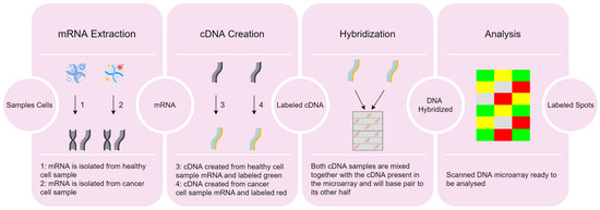
Figure 1. Overview of the DNA microarray technique data acquisition from samples [4].

1.

Extraction of ribonucleic acid (RNA) from the sample cells and drawing out the messenger RNA (mRNA) from the existing RNA, because only the mRNA develops gene expression.

2.

CDNA creation: a DNA copy is made from the mRNA using the reverse transcriptase enzyme, which generates the complementary DNA (CDNA). A label is added in the CDNA representing each cell sample (e.g., with fluorescent red and green for cancer and healthy cells, respectively). This step is necessary since DNA is more stable than RNA and this labeling allows identifying the genes.

3.

Hybridization: both CDNA types are added to the DNA microarray and each spot already has many unique CDNA. When mixed together, they will base-pair each other due to the DNA complementary base pairing property. Not all CDNA strands will bind to each other, since some may not hybridize being washed off.

4.

Analysis: the DNA microarray is analyzed with a scanner to find patterns of hybridization by detecting the fluorescent colors.

The following are possible outcomes of the analysis stage:

• A few red CDNA molecules bound to a spot, if the gene is expressed only in the cancer (red) cells;
• A few green CDNA molecules bound to another spot, if the gene is expressed only in the healthy (green) cells;
• Some of both red and green CDNA molecules bound to a single spot on the microarray, yielding a yellow spot; in this case, the gene is expressed both in the cancer and healthy cells;
• Finally, several spots of the microarray do not have a single red or green CDNA strand bound to them; this happens if the gene is not being expressed in either type of cell.

On the one hand, the red color flags the higher production of mRNA in the cancer cell as compared to the healthy cell. On the other hand, the green color states that we have a larger production of mRNA in the healthy cell, as compared to the cancer cell. However, a yellow spot suggests that the gene is expressed equally in both cells and therefore it is not related with the disease, because when the healthy cell becomes cancerous its activity does not change.

Figure 2 depicts the process of generating a dataset using the DNA microarray technique summarized in Figure 1.

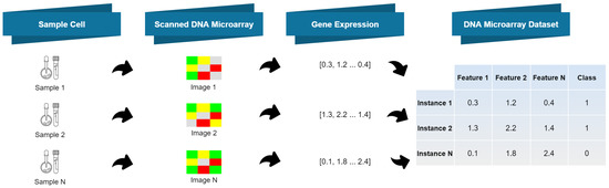
Figure 2. Dataset generation with gene expression data from DNA microarray data acquisition [4].

2.2. Feature Discretization

DNA microarray datasets are composed of high dimensionality numeric feature vectors. These features contain a large amount of information regarding gene expressions, but they also contain irrelevant fluctuations (noise) [10], which may be harmful for the performance of ML algorithms. The use of FD techniques, which convert continuous (numeric) features into discrete ones, may yield compact and adequate representations of the microarray data, with less noise [11,12]. In other words, FD aims at finding a representation of each feature that contains enough information for the learning task at hand, while ignoring minor fluctuations that may be irrelevant for the task at hand. FD methods can be supervised or unsupervised, depending on whether label information is used or not, respectively [11].

The Equal Frequency Binning (EFB) method [13], which is unsupervised, discretizes continuous features into a given number of intervals (bins), which contain approximately the same number of instances. The Unsupervised Linde-Buzo-Gray 1 (U-LBG1) method discretizes each feature into a specified number of intervals, by minimizing the Mean Squared Error (MSE) between the original and the discretized feature. The number of intervals may be decided by demanding that the MSE be lower than some threshold ($\Delta$) or by specifying the maximum number of bits per feature (q).

The supervised Minimum Description Length Principle (MDLP) method recursively divides the feature values into multiple intervals, using an information gain minimization heuristic (entropy). Please refer to [14] for a formal description of this method and to [5,13] for additional insights on other FD approaches.

2.3. Feature Selection

In the presence of high-dimensional data, dimensionality reduction techniques [9,15] are often essential to obtain adequate representations of the data and to improve the ML models results, effectively addressing the “curse of dimensionality”. One type of dimensionality reduction technique that has been successful with microarray data is FS [9,15]. FS techniques select a subset of features from the original set by following some selection criterion. One way to perform FS is to rank the features according to their relevance, assessed by a given function, which can also be supervised (if it uses label information) or not. For microarray data, the use of FS techniques is also known as Gene Selection (GS). Some well-known methods that have been used for microarray data are the following:

• Unsupervised methods—Laplacian Score (LS) [16], spectral (also known as SPEC) [17], and term-variance [18];
• Supervised methods—Fisher Ratio (FiR) [19], Fast Correlation-Based Filter (FCBF) [20], Maximum Relevance Minimum Redundancy (MRMR) [21], ReliefF [22], and Relevance-Redundancy Feature Selection (RRFS) [23].

The RRFS method can also work in unsupervised mode using the mean-median (MM) relevance metric, defined, for the i-th feature, as 

$${\mathrm{MM}}_i=|{\overline{X}}_i-\mathrm{median}\left(X_i\right)|,$$

(1)

with ${\overline{X}}_i$ denoting the mean of the i-th feature. In supervised mode, RRFS uses as relevance measure the Fisher ratio [19], also known as Fisher score, defined as (for the i-th feature)

$${\mathrm{FiR}}_i=\frac{\left|{\overline{X}}_i^{(-1)}-{\overline{X}}_i^{\left(1\right)}\right|}{\sqrt{\mathrm{var}{\left(X_i\right)}^{(-1)}+\mathrm{var}{\left(X_i\right)}^{\left(1\right)}}},$$

(2)

where ${\overline{X}}_i^{(-1)}$, ${\overline{X}}_i^{\left(1\right)}$, $\mathrm{var}{\left(X_i\right)}^{(-1)}$, and $\mathrm{var}{\left(X_i\right)}^{\left(1\right)}$, are the sample means and variances of feature $X_i$, for the patterns of each of the two classes (denoted as $-1$ and 1). This ratio measures how well each feature alone separates the two classes [19], and has been found to serve well as a relevance criterion for FS tasks. For  more than two classes, FiR for feature $X_i$ is generalized [6,24] as

$${\mathrm{FiR}}_i=\frac{{\displaystyle \sum _{j=1}^c{\mathrm{n}}_j{\left({\overline{X_i}}^{\left(j\right)}-\overline{X_i}\right)}^2}}{{\displaystyle \sum _{j=1}^c{\mathrm{n}}_j\mathrm{var}\left(X_i^{\left(j\right)}\right)}},$$

(3)

where c is the number of classes, $n_j$ is the number of samples in class j, and ${\overline{X_i}}^{\left(j\right)}$ denotes the sample mean of $X_i$, considering only samples in class j; finally, $\overline{X_i}$ is the sample mean of feature $X_i$. Among many other applications, the Fisher ratio has been used successfully with microarray data, as reported by Furey et al. [25]. When using the Fisher ratio for FS, we simply keep the top-rank features.

Recent surveys on FS techniques can be found in [26,27,28]. The use of FS techniques for microarray and related data is surveyed in [29,30,31,32].

2.4. Classifiers

In this section, we briefly review two successful classifiers, commonly used for microarray data: support vector machines (SVM) and decision trees (DT).

2.4.1. SVM

SMVs [33,34,35,36] follow a discriminative approach to learn a linear classifier. As is well-known, a non-linear SVM classifier can be obtained by the use of a kernel, via the so-called kernel trick [33]: since the SVM learning algorithm only uses inner products between feature vectors, these inner products can be replaced by kernel computations, which are equivalent to mapping those feature vectors into a high-dimensional (maybe non-linear) feature space. With a separable dataset, a SVM is learned by looking for the maximum-margin hyperplane (a linear model) that separates the instances according to their labels. In the non-separable case, this criterion is relaxed via the use of slack variables, which allow for the (penalized) violation of the margin constraint; for details, see [35,36]. SVMs are well suited for high-dimensional problems, such as the ones addressed in this paper. Although the original SVM formulation is inherently two-class (binary), different techniques have been proposed to generalize SVM to the multi-class case, such as one-vs-rest (or “one-versus-all”) and one-vs-one [37,38]. We have chosen the SVM classifier because it has been reported in the literature to yield the best results on this type of data.

2.4.2. DT

DT classifiers [33] also adopt a discriminative approach. A DT is a hierarchical model, in which each local region of the data is classified by a sequence of recursive splits, using a small number of partitions. The DT learning algorithm analyzes each (discrete or numeric) feature for all possible partitions and choose the one that maximizes one of the so-called impurity measures. The tree construction proceeds recursively and simultaneously for all branches that are not yet pure enough. The tree is complete when all the branches are considered pure enough, that is, when performing more splits does not improve the purity, or when the purity exceeds some threshold. There are several algorithms to learn a DT. The most popular are the Classification and Regression Trees (CART) [39], the ID3 algorithm [40] and its extension, the well-known C4.5 [41,42] algorithm. A survey of methods for constructing DT classifiers can be found in [43], which proposes a unified algorithmic framework for DT learning and describes different splitting criteria and tree pruning methods. DT are able to effectively handle high-dimensional and multi-class data. We have chosen DT because it is a different classification approach, which has seldom been applied to this type of data and provides intrinsically explainable classifiers.

2.5. Related Approaches

Many unsupervised and supervised FD and FS techniques have been employed on microarray data classification for cancer diagnosis [1,44,45]. Since microarray datasets are typically labeled, the use of supervised techniques is preferred, as supervised methods normally outperform unsupervised ones.

Some unsupervised FD techniques perform well when combined with some classifiers. For instance, the Equal Frequency Binning (EFB) technique followed by a Naïve Bayes (NB) classifier produces very good results [46]. It has also been reported that applying Equal Interval Binning (EIB) and EFB with microarray data, followed by SVM classifiers, yields good results [47]. It has also been shown that FS significantly improves the classification accuracy of multi-class SVM classifiers and other classification algorithms [48].

An FS filter (i.e., a FS method that is agnostic to the choice of classifier that will be subsequently used) for microarray data, based on the information-theoretic criterion named Double Input Symmetrical Relevance (DISR) was proposed by [47]. The DISR criterion is found to be competitive with existing unsupervised FS filters.

The work in [49] explores FS techniques, such as backward elimination of features, together with classification using Random Forest (RF) [50]. The authors concluded that RF has better performance than other classification methods, such as Diagonal Linear Discriminant Analysis (DLDA), K-Nearest Neighbors (KNN), and SVM. They also showed that their FS technique led to a smaller subset of features than alternative techniques, namely Nearest Shrunken Centroids (NSC) and a combination of filter and nearest neighbor classifier.

The work in [51] introduced the use of Large-scale Linear Support Vector Machine (LLSVM) and Recursive Feature Elimination with Variable Step Size (RFEVSS), improving the Recursive Feature Elimination (SVMRFE) technique. The improvement upgrades RFE with a variable step size, to reduce the number of iterations (in the initial stages in which non-relevant features are discarded, the step size is larger). The standard SVM is upgraded to a large-scale linear SVM, thus accelerating the method of assigning weights. The authors assess their approach to FS with SVM, RF, NB, KNN, and Logistic Regression (LR) classifiers. They conclude that their approach achieves comparable levels of accuracy, showing that SVM and LR outperform the other classifiers.

Recently, in the context of cancer explainability, the work in [52] considered the problem of finding a small subset of features to distinguish among six classes. The goal was to devise a set of rules based on the most relevant features that can distinguish classes based on their gene expressions. The proposed method combines a FS-based Genetic Algorithm (GA) with a fuzzy rule-based system to perform classification on a dataset with 21 instances, more than 45,000 features, and six classes. The proposed method generates ten rules, with each one addressing some specific features, making them crucial in explaining the classification results of ovarian cancer detection.

A survey of common classification techniques and related methods to increase their accuracy for microarray analysis can be found in [1,44]. The experimental evaluation is carried out in publicly available datasets. The work in [53] surveys the use of FS techniques for microarray data. For other related surveys, please see [51,54,55,56].

3. Proposed Approach

In this section, we describe our approach to DNA microarray classification with FD and FS. Section 3.1 describes the key characteristics of the public domain datasets used in the experimental evaluation. Section 3.2 details the pipeline of techniques we apply to the data, as well as the procedures that we follow. Finally, Section 3.3 describes the metrics used in our experimental evaluation.

3.1. Microarray Datasets and Clinical Tasks

Table 1 summarizes the main characteristics of the 11 microarray datasets considered in this work [57], available at (https://csse.szu.edu.cn/staff/zhuzx/Datasets.html, accessed on 2 July 2023). In this table, n denotes the number of instances, d indicates the number of features, and c the number of classes. We also show the $d/n$ ratio as well as the number of instances in each class. Finally, we display the number of numeric and categorical/nominal features in each dataset.

Table 1. Microarray datasets: n is the number of instances, d is the number of features, and c is the number of classes. Also shown are the number of instances per class and the number of numeric and categorical features.

Name	n	d	$\mathbf{d}/\mathbf{n}$	c	Instances per Class	Numeric, Categorical
Breast [58]	97	24,481	252.38	2	46, 51	24,188, 293
CNS [59]	60	7129	118.81	2	39, 21	7129, 0
Colon [60]	62	2000	32.25	2	40, 22	2000, 0
Leukemia [61]	72	7129	99.01	2	47, 25	7129, 0
Leukemia_3c [61]	72	7129	99.01	3	38, 25, 9	7129, 0
Leukemia_4c [61]	72	7129	99.01	4	38, 21, 9, 4	7129, 0
Lung [62]	203	12,600	62.06	5	139, 17, 6, 21, 20	12600, 0
Lymphoma [63]	66	4026	61.00	3	46, 11, 9	4026, 0
MLL [64]	72	12,582	174.75	3	28, 24, 20	11,270, 1312
Ovarian [65]	253	15,154	59.89	2	162, 91	15,151, 3
SRBCT [66]	83	2308	27.80	4	29, 11, 18, 25	2308, 0

These datasets have many more features than instances, $n\ll d$, which creates a challenge in applying ML techniques due to the curse of dimensionality [2,6]. The datasets have a large number of features (with d ranging from 2000 to 24,481). In addition, all datasets have a small number of instances (with n ranging from 60 to 253). For some datasets, we also have class imbalances. Table 2 details the classification task for each dataset presented in Table 1.

Table 2. Microarray dataset clinical tasks regarding cancer detection [4].

Name	Clinical Task Regarding Cancer Detection
Breast	Breast cancer diagnosis
CNS	Central Nervous System tumor diagnosis
Colon	Colon tumor diagnosis
Leukemia	Acute Lymphocytic Leukemia and
	Acute Myelogenous Leukemia diagnosis
Leukemia_3c	Distinguishes types of blood cells which became cancerous
Leukemia_4c	Distinguishes types of blood cells which became cancerous
Lung	Lung cancer diagnosis
Lymphoma	Distinguishes subtypes of non-Hodgkin lymphoma
MLL	Distinguishes types of acute leukemia, including
	Mixed Lineage Leukemia
Ovarian	Ovarian cancer diagnosis
SRBCT	Distinguishes types of of Small Round Blue Cell Tumors

In the datasets with two classes, we have the following binary classification tasks:

• Detecting the presence of a specific cancer (such as in CNS, Colon, and Ovarian);
• Detecting the re-incidence of a disease (Breast dataset);
• Diagnosing between two types of cancer (Leukemia dataset).

The multi-class datasets address the following problems:

• Distinguishing among different types of cells (Leukemia_3c, Leukemia_4c, and Lymphoma);
• Distinguishing between healthy situation and the presence of cancer (Lung, MLL, and SRBCT).

3.2. Machine Learning Pipeline

Our proposal combines FD and FS techniques before classification. Our aim is to attain low classification error rate, false negative rate, and false positive rate. Moreover, we also intend to find the smallest subsets of features that are most relevant for each classification task. In detail, the steps of our approach are:

• Choosing the techniques under evaluation;
• Building a ML pipeline using data representation/discretization, dimensionality reduction, and data classification techniques;
• Comparing the performance of these techniques, using standard metrics;
• Identifying, for each dataset, the best technique as well as the best subset of features.

Figure 3 summarizes the pipeline proposed in this paper, while Algorithm 1 describes this ML pipeline in a more formal way.

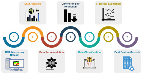
Figure 3. The detailed stages taken in this study [4], numbered from (1) to (7).

In line 2 of Algorithm 1, we preprocess each dataset, which includes the following key steps:

1.

Mapping all nominal class labels to a number (for instance: no cancer corresponds to 0, whereas cancer corresponds to 1); this is performed because some algorithms do not accept nominal labels.

2.

Filling the missing values with the most frequent value in the corresponding feature. We used the SimpleImputer method from Scikit-learn. This is only required for the Lymphoma dataset, as it was the only one with missing values.

3.

Removing constant features, since they provide no information for classification. This is only required for the Breast dataset, in which d is reduced from 24,481 to 24,188.

In line 3, we instantiate and initialize the LOO (leave-one-out) procedure for training and testing classifiers, which is then applied to all evaluations throughout. By using LOO, we achieve a better estimate of the generalization error and the other evaluation metrics, when compared to standard 10-fold cross validation (CV). Since the number of instances n is small, it is preferable to resort to LOOCV.

In line 12, we count how many times a feature is selected in the FS stage of the pipeline. Since we are using a LOO scheme, each feature can be selected from 0 to n times. We sort these counters in descending order, and take their values as a measure of feature relevance. This way, we implement stage (7) of the pipeline. The code for the experimental part of this work is written in Python (version 3.7) and resorts to Scikit-learn and other standard packages, such as Pandas, Numpy, and Scipy. The code and the datasets are available at (https://github.com/adaranogueira/cancer-diagnosis-ml, accessed on 2 July 2023).

Algorithm 1 Machine learning pipeline

Input:     11 DNA microarray datasets, described in Table 1.

Output:   Error rate (Err). False negative rate (FNR). False positive rate (FPR). Percentage of the selected features ($m^{\prime }$).

1: for$data\in datasets$do     2:    Preprocess the data.     3:    Initialize the leave-one-out cross validation (LOOCV) procedure.     4:    for each LOOCV fold do     5:      Split the instances of the data into training and test sets.     6:      Apply feature normalization (scaling to the 0 to 1 range) on each feature on the training and test sets.     7:      for $fd\in FDtechniques$ do     8:         Apply stage (3) as depicted in Figure 3     9:         for $fs\in FStechniques$ do     10:           Apply stage (4).     11:           Select features on the discretized training and test sets.     12:           Compute how many times a feature was selected.     13:           for $classifier\in classificationtechniques$ do     14:              Apply stage (5).     15:              Save the classifier predictions (stage (6))     16:           end for     17:         end for     18:      end for     19:    end for     20: end for     21: For all datasets and combinations of techniques applied in this pipeline, compute the confusion matrix using the saved predictions (stage (6)).     22: Compute Err, FNR, and FPR using the confusion matrix.     23: Compute $m^{\prime }$, the percentage of selected features.

3.3. Evaluation Metrics

We now describe the metrics employed for performance evaluation. In this context, we consider that a positive prediction relates to cancer while a negative prediction is the absence of cancer. The well-known metrics true negative (TN), true positive (TP), false positive (FP), and false negative (FN) are considered. The accuracy (Acc) and error rate (Err) measures the proportion of, respectively, correct and incorrect classifications out of all predictions. These two rates satisfy the well-known relation Err = 1 − Acc. The False Negative Rate (FNR) is the proportion of actual positive instances that are incorrectly identified as negative, while the False Positive Rate (FPR) is the proportion of negative instances that are incorrectly identified as positive. Besides the accuracy, the most important metric in this type of data is the FNR. In most medical applications, the cost of a FN is usually much higher than that of a FP, since it can correspond to failing to detect a disease, which can cause harm or even death.

4. Experimental Evaluation

This section reports the experimental evaluation of the proposed ML pipeline, depicted in Figure 3. The section is organized as follows:

• Section 4.1 addresses the baseline classification results without FD and FS, using the SVM and DT classifiers (stages (1), (2), (5), and (6) of the pipeline).
• Section 4.2 refers to the use of FD techniques (stages (1), (3), (5), and (6) of the pipeline).
• Section 4.3 reports the experimental results of FS techniques (stages (1), (4), (5), and (6) of the pipeline).
• Section 4.4 summarizes the best ML pipeline configuration found for each dataset.
• Section 4.5 reports the experimental results towards the explainability of the classification (stage (7)). We show the subsets of features that are most often chosen for each dataset.

4.1. Baseline Classification Results: Stages (1), (2), (5), and (6)

First, we address only the classification stage of the pipeline, by assessing the performance of SVM and DT classifiers, providing the baseline results. We follow the LOOCV procedure for all the evaluations reported in this paper. Since the number of instances n is small, we achieve better estimates of the several evaluation metrics, as compared to the use of standard 10-fold CV. In LOOCV, we have no standard deviation on the experimental metrics, due to the data sampling procedure.

Table 3 presents the baseline results (no FD nor FS) with stage (b) of the pipeline being the normalization of all feature values to the range 0 to 1. Table 4 shows a similar evaluation for the DT classifier. In our experiments, we have found that using entropy as a criterion to build the tree is better than using the Gini index; we have also found that the initial random_state parameter set to 42 is the best choice.

Table 3. Test error rate (Err) of LOOCV for the SVM classifier with different kernels. For five datasets that have a class label of “no cancer”, we also consider the False Negative Rate (FNR) and False Positive Rate (FPR) metrics. For the other six datasets, we do not report the FNR and FPR metrics, because the task is to distinguish between cancer types. The best result is in boldface [4].

	Linear Kernel			Poly Kernel			RBF Kernel			Sigmoid Kernel
Dataset	Err	FNR	FPR	Err	FNR	FPR	Err	FNR	FPR	Err	FNR	FPR
Breast	0.31	0.30	0.31	0.33	0.28	0.37	0.37	0.46	0.29	0.47	1.00	0.00
CNS	0.33	0.62	0.18	0.37	0.62	0.23	0.35	1.00	0.00	0.35	1.00	0.00
Colon	0.18	0.27	0.12	0.27	0.55	0.12	0.21	0.50	0.05	0.39	0.82	0.15
Leukemia	0.01	–	–	0.03	–	–	0.15	–	–	0.35	–	–
Leukemia_3c	0.04	–	–	0.06	–	–	0.26	–	–	0.47	–	–
Leukemia_4c	0.07	–	–	0.10	–	–	0.32	–	–	0.47	–	–
Lung	0.05	0.01	0.12	0.05	0.01	0.18	0.09	0.01	0.24	0.32	0.00	1.00
Lymphoma	0.00	–	–	0.00	–	–	0.00	–	–	0.30	–	–
MLL	0.03	–	–	0.06	–	–	0.10	–	–	0.61	–	–
Ovarian	0.00	0.00	0.00	0.004	0.00	0.01	0.02	0.01	0.02	0.36	0.00	1.00
SRBCT	0.00	–	–	0.01	–	–	0.07	–	–	0.65	–	–
Average	0.09	0.24	0.15	0.12	0.29	0.18	0.18	0.40	0.12	0.43	0.56	0.43
Std. dev.	0.12	0.23	0.10	0.13	0.26	0.12	0.13	0.37	0.12	0.11	0.47	0.47

Table 4. Test error rate (Err), FNR, and FPR of LOOCV for the DT classifier using entropy as criterion and random_state set to 42, with normalized features in the range 0 to 1. Different values for the max_depth parameter are evaluated (the learned tree maximum allowed depth). The best result is in boldface [4].

	Max Depth = 2			Max Depth = 5			Max Depth = 7			Max Depth = 10
Dataset	Err	FNR	FPR	Err	FNR	FPR	Err	FNR	FPR	Err	FNR	FPR
Breast	0.40	0.35	0.45	0.33	0.30	0.35	0.33	0.30	0.35	0.33	0.30	0.35
CNS	0.18	0.48	0.03	0.25	0.33	0.21	0.25	0.33	0.21	0.25	0.33	0.21
Colon	0.18	0.36	0.08	0.19	0.23	0.18	0.19	0.23	0.18	0.19	0.23	0.18
Leukemia	0.26	–	–	0.26	–	–	0.26	–	–	0.26	–	–
Leukemia_3c	0.15	–	–	0.17	–	–	0.17	–	–	0.17	–	–
Leukemia_4c	0.11	–	–	0.15	–	–	0.15	–	–	0.15	–	–
Lung	0.13	0.01	0.06	0.07	0.01	0.12	0.07	0.01	0.12	0.07	0.01	0.12
Lymphoma	0.00	–	–	0.00	–	–	0.00	–	–	0.00	–	–
MLL	0.08	–	–	0.08	–	–	0.08	–	–	0.08	–	–
Ovarian	0.03	0.01	0.07	0.03	0.01	0.07	0.03	0.01	0.07	0.03	0.01	0.07
SRBCT	0.27	–	–	0.17	–	–	0.17	–	–	0.17	–	–
Average	0.16	0.24	0.14	0.15	0.18	0.19	0.15	0.18	0.19	0.15	0.18	0.19
Std. dev.	0.11	0.19	0.16	0.10	0.14	0.10	0.10	0.14	0.10	0.10	0.14	0.10

The experimental results in Table 3 and Table 4 show that DT does not achieve better results than the SVM classifier (the DT classifier outperforms SVM only on the CNS dataset). Thus, from these experiments and from the existing literature, a SVM with a linear kernel seems to be an adequate classifier for this type of data. From these experiments, we have also found that it is advantageous to normalize the data before addressing any machine learning tasks.

4.2. Feature Discretization Assessment: Stages (1), (3), (5), and (6)

In the literature on microarray data, the unsupervised EFB method has been reported to produce good results. Thus, we have carried out some experiments using this FD method. Table 5 reports the results of the SVM classifier on data discretized by EFB, with different numbers of bins. The results in this table show that EFB discretization yields a small improvement with the SVM classifier (lower standard deviation in all datasets). Table 6 shows a summary of the results of the best configurations of EFB discretization and SVM/DT classifiers. For each dataset, we select the best configuration found in our experiments. Table 7 shows a similar experiment as in Table 6, but now for the DT classifier. These results show that DT classifiers also benefit from FD, with five bits yielding the lowest error rate.

Table 5. Test error rate (Err), FNR, and FPR of LOOCV for the SVM classifier (C = 1 and kernel = linear) with EFB discretization. Different values for the n_bins parameter were evaluated (the number of discretization bins). The best result is in boldface [4].

	Num. Bins = 2			Num. Bins = 3			Num. Bins = 4			Num. Bins = 5			Num. Bins = 6			Num. Bins = 7
Dataset	Err	FNR	FPR	Err	FNR	FPR	Err	FNR	FPR	Err	FNR	FPR	Err	FNR	FPR	Err	FNR	FPR
Breast	0.32	0.30	0.33	0.33	0.33	0.33	0.32	0.33	0.31	0.32	0.33	0.31	0.30	0.30	0.29	0.31	0.33	0.29
CNS	0.35	0.71	0.15	0.30	0.62	0.13	0.38	0.71	0.21	0.32	0.62	0.15	0.32	0.62	0.15	0.37	0.67	0.21
Colon	0.18	0.27	0.12	0.18	0.27	0.12	0.16	0.27	0.10	0.15	0.23	0.10	0.15	0.23	0.10	0.16	0.27	0.10
Leukemia	0.01	–	–	0.01	–	–	0.01	–	–	0.01	–	–	0.01	–	–	0.01	–	–
Leukemia_3c	0.03	–	–	0.03	–	–	0.03	–	–	0.03	–	–	0.04	–	–	0.04	–	–
Leukemia_4c	0.08	–	–	0.07	–	–	0.07	–	–	0.07	–	–	0.07	–	–	0.07	–	–
Lung	0.05	0.01	0.18	0.05	0.01	0.18	0.05	0.01	0.18	0.04	0.01	0.18	0.04	0.01	0.18	0.04	0.01	0.18
Lymphoma	0.00	–	–	0.00	–	–	0.00	–	–	0.00	–	–	0.00	–	–	0.00	–	–
MLL	0.04	–	–	0.03	–	–	0.03	–	–	0.03	–	–	0.03	–	–	0.03	–	–
Ovarian	0.004	0.00	0.01	0.00	0.00	0.00	0.00	0.00	0.00	0.00	0.00	0.00	0.00	0.00	0.00	0.00	0.00	0.00
SRBCT	0.00	–	–	0.00	–	–	0.00	–	–	0.00	–	–	0.00	–	–	0.00	–	–
Average	0.10	0.26	0.16	0.09	0.25	0.15	0.10	0.26	0.16	0.09	0.24	0.15	0.09	0.23	0.14	0.09	0.26	0.16
Std. dev.	0.12	0.26	0.10	0.12	0.23	0.11	0.13	0.26	0.10	0.12	0.23	0.10	0.11	0.23	0.10	0.12	0.25	0.10

Table 6. Summary of the best results and corresponding configurations, for each dataset with normalized features, obtained during the data representation stage with the EFB discretizer. The * symbol denotes an improvement over the baseline classification results of Table 3 and Table 4, without discretization [4].

		Configurations
Dataset	Classifier	Num. Bins	Err	FNR	FPR
Breast	SVM	6	0.30 *	0.30	0.29
CNS	DT	5	0.18	0.33	0.10
Colon	SVM	5, 6	0.15 *	0.23	0.10
Leukemia	SVM, DT	2, 3, 4, 5, 6, 7	0.01	–	–
Leukemia_3c	SVM	2, 3, 4, 5	0.03 *	–	–
Leukemia_4c	SVM	3, 4, 5, 6, 7	0.07 *	–	–
Lung	SVM	5, 6, 7	0.04 *	0.01	0.18
Lymphoma	SVM	2, 3, 4, 5, 6, 7	0.00	–	–
MLL	SVM	3, 4, 5, 6, 7	0.03	–	–
Ovarian	SVM	3, 4, 5, 6, 7	0.00	0.00	0.00
SRBCT	SVM	2, 3, 4, 5, 6, 7	0.00	–	–
Average	–	–	0.07	0.17	0.13
Std. dev.	–	–	0.09	0.14	0.10

Table 7. Test error rate (Err), FNR, and FPR of LOOCV for the DT classifier (criterion = entropy, max_depth = 5, and random_state = 42) with EFB discretization. Different values for the n_bins parameter were evaluated. The best results are presented in boldface.

	2			3			4			5			6			7
Dataset	Err	FNR	FPR	Err	FNR	FPR	Err	FNR	FPR	Err	FNR	FPR	Err	FNR	FPR	Err	FNR	FPR
Breast	0.30	0.35	0.25	0.30	0.35	0.25	0.46	0.50	0.43	0.32	0.37	0.27	0.47	0.59	0.37	0.48	0.61	0.37
CNS	0.42	0.67	0.28	0.65	0.81	0.56	0.43	0.57	0.36	0.18	0.33	0.10	0.37	0.57	0.26	0.50	0.71	0.38
Colon	0.26	0.32	0.22	0.34	0.55	0.22	0.29	0.55	0.15	0.16	0.18	0.15	0.34	0.45	0.28	0.24	0.41	0.15
Leukemia	0.01	–	–	0.11	–	–	0.12	–	–	0.19	–	–	0.08	–	–	0.14	–	–
Leukemia_3c	0.19	–	–	0.22	–	–	0.12	–	–	0.14	–	–	0.10	–	–	0.19	–	–
Leukemia_4c	0.21	–	–	0.28	–	–	0.10	–	–	0.26	–	–	0.21	–	–	0.17	–	–
Lung	0.27	0.07	0.47	0.17	0.01	0.12	0.16	0.02	0.12	0.15	0.03	0.41	0.18	0.05	0.35	0.15	0.03	0.29
Lymphoma	0.06	–	–	0.06	–	–	0.11	–	–	0.09	–	–	0.09	–	–	0.11	–	–
MLL	0.19	–	–	0.17	–	–	0.25	–	–	0.15	–	–	0.08	–	–	0.18	–	–
Ovarian	0.06	0.07	0.03	0.02	0.01	0.03	0.04	0.04	0.03	0.03	0.01	0.05	0.02	0.01	0.04	0.03	0.01	0.07
SRBCT	0.18	–	–	0.25	–	–	0.22	–	–	0.16	–	–	0.23	–	–	0.17	–	–
Average	0.20	0.30	0.25	0.23	0.35	0.24	0.21	0.34	0.22	0.17	0.18	0.20	0.20	0.33	0.26	0.21	0.35	0.25
Std. dev.	0.11	0.22	0.14	0.16	0.31	0.18	0.13	0.25	0.15	0.07	0.15	0.13	0.14	0.25	0.12	0.14	0.29	0.12

Figure 4 shows the connection between the average error rate of all datasets and the number of discretization bins, for the SVM and DT classifiers.

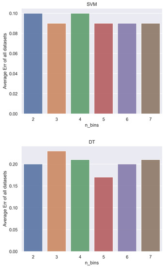
Figure 4. Analysis of the error rate (Err) and number of discretization bins (n_bins) for the SVM classifier (top) and the DT classifier (bottom).

We can observe the increasing and decreasing effect regarding the improvements on the classifiers performance. For the SVM classifier, the optimal n_bins is 6 (lower error and lower standard deviation) whereas for the DT classifier, the optimal value is n_bins = 5.

4.3. Feature Selection Assessment: Stages (1), (4), (5), and (6)

We now address the use of FS on the normalized features (without FD). For our experiments, we consider the Laplacian Score (LS), Spectral, Fisher Ratio (FiR), and Relevance-Redundancy Feature Selection (RRFS) [23]. Table 8 shows the experimental results for the SVM classifier, while Table 9 shows the results of the DT classifier. RRFS works in unsupervised mode using the MM relevance metric and in supervised mode with FiR as metric.

Table 8. Test error rate (Err), FNR, and FPR of LOOCV for the SVM classifier (C = 1 and kernel = linear) with LS, SPEC, FiR, and RRFS (with MM and FiR relevance and maximum similarity $m_s$ = 0.7), with normalized features. The best result is in boldface [4].

	Unsupervised									Supervised
	LS			SPEC			RRFS (MM)			FiR			RRFS (FiR)
Dataset	Err	FNR	FPR	Err	FNR	FPR	Err	FNR	FPR	Err	FNR	FPR	Err	FNR	FPR
Breast	0.33	0.35	0.31	0.32	0.30	0.33	0.31	0.28	0.33	0.31	0.28	0.33	0.31	0.28	0.33
CNS	0.35	0.52	0.26	0.33	0.62	0.18	0.27	0.48	0.15	0.30	0.57	0.15	0.33	0.67	0.15
Colon	0.16	0.27	0.10	0.19	0.32	0.12	0.21	0.36	0.12	0.19	0.32	0.12	0.18	0.27	0.12
Leukemia	0.01	–	–	0.01	–	–	0.01	–	–	0.01	–	–	0.01	–	–
Leukemia_3c	0.04	–	–	0.06	–	–	0.04	–	–	0.04	–	–	0.03	–	–
Leukemia_4c	0.08	–	–	0.10	–	–	0.07	–	–	0.07	–	–	0.07	–	–
Lung	0.05	0.01	0.12	0.05	0.01	0.12	0.05	0.01	0.12	0.04	0.01	0.12	0.05	0.01	0.18
Lymphoma	0.00	–	–	0.00	–	–	0.03	–	–	0.00	–	–	0.02	–	–
MLL	0.04	–	–	0.06	–	–	0.03	–	–	0.03	–	–	0.04	–	–
Ovarian	0.00	0.00	0.00	0.00	0.00	0.00	0.004	0.00	0.01	0.00	0.00	0.00	0.00	0.00	0.00
SRBCT	0.02	–	–	0.00	–	–	0.00	–	–	0.00	–	–	0.00	–	–
Average	0.10	0.23	0.16	0.10	0.25	0.15	0.09	0.23	0.15	0.09	0.24	0.14	0.09	0.25	0.16
Std. dev.	0.12	0.20	0.11	0.12	0.23	0.11	0.11	0.19	0.10	0.11	0.21	0.11	0.12	0.24	0.11

Table 9. Test error rate (Err), FNR, and FPR of LOO for the DT classifier (criterion = entropy, max_depth = 5, and random_state = 42) with LS, SPEC, FiR, and RRFS (with MM and FiR relevance and $ms$ = 0.7). The best results are presented in boldface.

	Unsupervised									Supervised
	LS			SPEC			RRFS (MM)			FiR			RRFS (FiR)
Dataset	Err	FNR	FPR	Err	FNR	FPR	Err	FNR	FPR	Err	FNR	FPR	Err	FNR	FPR
Breast	0.43	0.50	0.37	0.29	0.30	0.27	0.41	0.50	0.33	0.37	0.33	0.41	0.26	0.33	0.20
CNS	0.38	0.67	0.23	0.22	0.38	0.13	0.28	0.43	0.21	0.32	0.38	0.28	0.32	0.38	0.28
Colon	0.32	0.50	0.22	0.34	0.55	0.22	0.19	0.32	0.12	0.26	0.27	0.25	0.21	0.27	0.18
Leukemia	0.14	–	–	0.21	–	–	0.21	–	–	0.25	–	–	0.15	–	–
Leukemia_3c	0.07	–	–	0.14	–	–	0.14	–	–	0.17	–	–	0.15	–	–
Leukemia_4c	0.12	–	–	0.25	–	–	0.14	–	–	0.11	–	–	0.22	–	–
Lung	0.15	0.03	0.41	0.16	0.01	0.18	0.09	0.01	0.12	0.09	0.01	0.18	0.08	0.01	0.18
Lymphoma	0.23	–	–	0.18	–	–	0.08	–	–	0.08	–	–	0.12	–	–
MLL	0.26	–	–	0.26	–	–	0.14	–	–	0.07	–	–	0.15	–	–
Ovarian	0.04	0.02	0.08	0.04	0.04	0.05	0.02	0.02	0.02	0.03	0.02	0.04	0.02	0.01	0.04
SRBCT	0.23	–	–	0.20	–	–	0.17	–	–	0.23	–	–	0.17	–	–
Average	0.22	0.34	0.26	0.21	0.26	0.17	0.17	0.26	0.16	0.18	0.20	0.23	0.17	0.20	0.18
Std. dev.	0.12	0.27	0.12	0.08	0.21	0.08	0.10	0.20	0.10	0.11	0.16	0.12	0.08	0.16	0.08

The RRFS method attains the best classification error results, while also achieving considerable dimensionality reduction. For instance, in the Ovarian dataset, we obtain a reduction to 4% of the original dimensionality: the number of selected features is 606 out of the original 15,154 features. A similar result is obtained for the Lymphoma dataset, in which we keep only 2% of the original features.

Figure 5 shows the graphical representation of the error rate (for the SVM and DT classifiers) and the corresponding percentage of the selected features ($m^{\prime }$), for the FS methods considered in this work. We report the average error rates and the average number of selected features, from Table 8 and Table 9.

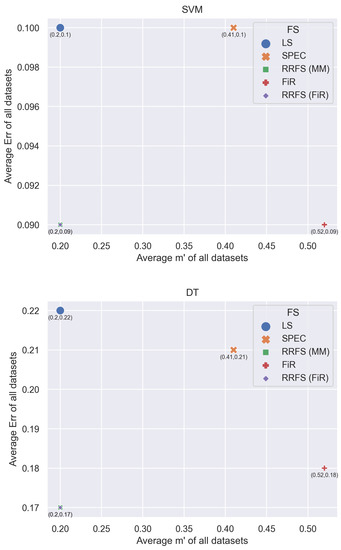
Figure 5. Average error rate (Err) and average percentage of selected features ($m^{\prime }$) for LS, SPEC, FiR, and RRFS (with MM and FiR; $ms$ = 0.7).

4.4. The Complete Pipeline: Best Configuration for Each Dataset

We now study the joint effect of all the pipeline stages depicted in Figure 3. Table 10 presents the best configurations for each stage and each dataset. Table 11 summarizes the best results obtained in this work for each dataset.

Table 10. Best pipeline configuration found for each dataset [4].

	Pipeline Configuration
Dataset	Discretization	Selection	Classification
Breast	EFB (n_bins = 6)	RRFS (with FiR; $ms$ = 0.7)	SVM (C = 1; kernel = linear)
CNS	EFB (n_bins = 5)	SPEC	DT (criterion = entropy, max_depth = 6, and random_state = 42)
Colon	MDLP	LS	DT (criterion = entropy, max_depth = None, and random_state = 5)
Leukemia	EFB (n_bins = 2)	LS	SVM (C = 1; kernel = linear)
Leukemia_3c	EFB (n_bins = 2)	RRFS (with FiR; $ms$ = 0.7)	SVM (C = 1; kernel = linear)
Leukemia_4c	EFB (n_bins = 3)	RRFS (with FiR; $ms$ = 0.7)	SVM (C = 1; kernel = linear)
Lung	EFB (n_bins = 5)	FiR	SVM (C = 1; kernel = linear)
Lymphoma	EFB (n_bins = 2)	LS	SVM (C = 1; kernel = linear)
MLL	EFB (n_bins = 3)	RRFS (with MM; $ms$ = 0.7)	SVM (C = 1; kernel = linear)
Ovarian	EFB (n_bins = 3)	RRFS (with FiR; $ms$ = 0.7)	SVM (C = 1; kernel = linear)
SRBCT	EFB (n_bins = 2)	SPEC	SVM (C = 1; kernel = linear)

Table 11. Summary of the best combination of techniques and their respective results for each dataset. Techniques: EFB (n_bins), RRFS (relevance metric, $ms$), SVM (C, kernel), and DT (criterion, max_depth, random_state).

	Configurations			Results
Dataset	Discretization	Selection	Classification	Err	FNR	FPR	${\mathit{m}}^{\prime }$
Breast	EFB (6)	–	SVM (1, linear)	0.30	0.30	0.29	–
CNS	EFB (5)	–	DT (entropy, 5, 42)	0.18	0.33	0.10	–
Colon	–	–	DT (entropy, None, 5)	0.13	0.23	0.08	–
Leukemia	–	LS	SVM (1, linear)	0.01	–	–	0.13
Leukemia_3c	–	RRFS (FiR, 0.7)	SVM (1, linear)	0.03	–	–	0.18
Leukemia_4c	–	RRFS (FiR, 0.7)	SVM (1, linear)	0.07	–	–	0.17
Lung	–	FiR	SVM (1, linear)	0.04	0.01	0.12	0.67
Lymphoma	–	LS	SVM (1, linear)	0.00	–	–	0.22
MLL	–	RRFS (MM, 0.7)	SVM (1, linear)	0.03	–	–	0.23
Ovarian	–	RRFS (FiR, 0.7)	SVM (1, linear)	0.00	0.00	0.00	0.04
SRBCT	–	SPEC	SVM (1, linear)	0.00	–	–	0.49

The conclusions of these experimental results can be summarized as follows. Based on the combination of techniques that yielded the best results, we observe that applying both FD and FS techniques did not improve the results in any dataset. For the Breast and CNS datasets, applying FS did not improve the results, but applying FD techniques did (the best result was achieved by applying the FD technique only). In addition, for the Colon dataset in particular, the best results were achieved by applying the baseline classifier to the original features (without FD or FS). For the remaining datasets, applying FS improved the results. In some cases, it improved the Err/FNR/FPR metrics, in other cases it was able to produce the same results with fewer features. In either case, the reduction of the number of features improved the explainability of the results and the time to compute them.

We have also found that DT does not achieve better results than the SVM classifier (DT performs better than SVM only on the CNS and Colon datasets). In addition, the EFB discretization also proved to be a better choice when compared to the MDLP technique. As for the FS techniques explored in this work, the RRFS method is in general the best choice, taking into account the classification error and the size of the subsets of features.

4.5. Explainability: Most Relevant Genes–Stage (7)

We further explore the use of the ML pipeline, aiming to identify the most decisive features for each dataset, since we have an acceptable error rate as reported in the previous sections. The rationale of this approach is the following:

• Use of the LOOCV procedure, which draws n data folds for training/testing;
• On a dataset with n instances, each feature can be chosen up to n times;
• The importance of a feature to accurately classify a dataset, on all data folds, and to explain the classification results is proportional to the number of times that feature is chosen;
• After the LOOCV procedure, we count the number of times each feature was chosen and we display the corresponding counters in decreasing order.

Figure 6 shows the top-20 feature indices that are chosen more often by the procedure mentioned above, for the Lymphoma, Ovarian, Leukemia, and SRBCT datasets, respectively.

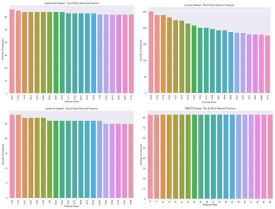
Figure 6. The top-20 of the number of times each feature is chosen/selected on the FS step on the LOOCV procedure for the Lymphoma (n = 66, d = 4026), Ovarian (n = 253, d = 15,154), Leukemia (n = 72, d = 7129), and SRBCT (n = 83, d = 2308) datasets.

For the Lymphoma and Ovarian datasets, only one feature is chosen n times. On the Lymphoma dataset, feature 1402 is chosen 66 times and on the Ovarian dataset, feature 1679 is chosen 253 times, which means that these features are always present in the classification decision. The feature indices shown on the xx-axis of these plots correspond to the most relevant features (genes) for cancer detection, which potentially contain clinically relevant information requiring further inspection by experts. As we move along the horizontal axis, we observe a decrease in the relative relevance of the features in the classification task.

Figure 7 displays the number of times each feature is chosen, for the Leukemia, Leukemia_3c, Leukemia_4c, and SRBCT datasets. These plots show that some features are chosen n times. However, on the Leukemia dataset, with $n=72$, we observe that no feature is chosen more than 28 times.

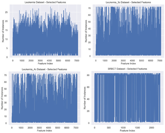
Figure 7. The number of times each feature is chosen/selected for the Leukemia (n = 72, d = 7129), Leukemia_3c (n = 72, d = 7129), Leukemia_4c (n = 72, d = 7129), and SRBCT datasets (n = 83, d = 2308).

5. Conclusions

The problem of cancer detection from DNA microarray data is a challenging machine learning problem, given the high-dimensionality of the data and the small number of instances usually available. However, over the years, some techniques have been successfully applied to this problem. Moreover, besides accurate data classification, the identification of the most relevant genes for the classification task is also an important goal, which clearly has important clinical information.

In this work, we have proposed an approach based on a machine learning pipeline, using a sequence of feature discretization and feature selection techniques, which is able to identify small subsets of relevant genes for the subsequent classifier. We consider standard machine learning procedures, achieving large degrees of dimensionality reduction on several public-domain datasets and identifying, for each dataset, the best combination of discretization, selection, classification techniques. Resorting to the leave-one-out cross validation procedure, we rank the features in decreasing order of importance for the classification task. Moreover, the comparison with the baseline classification error and false negative rates assures that we find the combination of techniques that performs better than the baseline. Our code and datasets are publicly available.

In future work, we will explore more supervised feature discretization and feature selection techniques. We will also fine-tune the maximum similarity parameter of the RRFS algorithm to further reduce the size of the subsets, allowing medical experts to focus on fewer features. Another research direction will be focused on the key limitation of this study, which is that the discretization and selection techniques work independently. Thus, we aim to devise a joint hybrid discretization and selection algorithm, suited for microarray data.

References

- Alonso-Betanzos, A.; Bolón-Canedo, V.; Morán-Fernández, L.; Sánchez-Marono, N. A Review of Microarray Datasets: Where to Find Them and Specific Characteristics. Methods Mol. Biol. 2019, 1986, 65–85. [Google Scholar] [CrossRef] [PubMed]
- Bishop, C. Neural Networks for Pattern Recognition; Oxford University: Oxford, UK, 1995. [Google Scholar]
- Hughes, G. On the mean accuracy of statistical pattern recognizers. IEEE Trans. Inf. Theory 1968, 14, 55–63. [Google Scholar] [CrossRef]
- Nogueira, A.; Ferreira, A.; Figueiredo, M. A Step Towards the Explainability of Microarray Data for Cancer Diagnosis with Machine Learning Techniques. In Proceedings of the International Conference on Pattern Recognition Applications and Methods (ICPRAM), Online, 3–5 February 2022; pp. 362–369. [Google Scholar] [CrossRef]
- Garcia, S.; Luengo, J.; Saez, J.; Lopez, V.; Herrera, F. A survey of discretization techniques: Taxonomy and empirical analysis in supervised learning. IEEE Trans. Knowl. Data Eng. 2013, 25, 734–750. [Google Scholar] [CrossRef]
- Duda, R.; Hart, P.; Stork, D. Pattern Classification, 2nd ed.; John Wiley & Sons: Hoboken, NJ, USA, 2001. [Google Scholar]
- Escolano, F.; Suau, P.; Bonev, B. Information Theory in Computer Vision and Pattern Recognition; Springer: Berlin/Heidelberg, Germany, 2009. [Google Scholar]
- Hastie, T.; Tibshirani, R.; Friedman, J. The Elements of Statistical Learning, 2nd ed.; Springer: Berlin/Heidelberg, Germany, 2009. [Google Scholar]
- Guyon, I.; Gunn, S.; Nikravesh, M.; Zadeh, L. Feature Extraction: Foundations and Applications; Springer: Berlin/Heidelberg, Germany, 2006. [Google Scholar]
- Simon, R.; Korn, E.; McShane, L.; Radmacher, M.; Wright, G.; Zhao, Y. Design and Analysis of DNA Microarray Investigations; Springer: New York, NY, USA, 2003. [Google Scholar]
- Ferreira, A.; Figueiredo, M. Exploiting the bin-class histograms for feature selection on discrete data. In Proceedings of the Iberian Conference on Pattern Recognition and Image Analysis, Santiago de Compostela, Spain, 17–19 June 2015; Springer: Cham, Switzerland, 2015; pp. 345–353. [Google Scholar]
- Belkin, M.; Niyogi, P. Laplacian eigenmaps for dimensionality reduction and data representation. Neural Comput. 2003, 15, 1373–1396. [Google Scholar] [CrossRef]
- Dougherty, J.; Kohavi, R.; Sahami, M. Supervised and unsupervised discretization of continuous features. In Machine Learning Proceedings 1995; Elsevier: Amsterdam, The Netherlands, 1995; pp. 194–202. [Google Scholar]
- Fayyad, U.; Irani, K. Multi-interval discretization of continuous-valued attributes for classification learning. In Proceedings of the International Joint Conference on Uncertainty in AI, Washington, DC, USA, 9–11 July 1993; pp. 1022–1027. [Google Scholar]
- Alpaydin, E. Introduction to Machine Learning, 3rd ed.; The MIT Press: Cambridge, MA, USA, 2014. [Google Scholar]
- He, X.; Cai, D.; Niyogi, P. Laplacian score for feature selection. In Proceedings of the Advances in Neural Information Processing Systems, Vancouver, BC, Canada, 5–8 December 2005; MIT Press: Cambridge, MA, USA; Volume 18, pp. 507–514. [Google Scholar]
- Zhao, Z.; Liu, H. Spectral feature selection for supervised and unsupervised learning. In Proceedings of the 24th International Conference on Machine Learning, Corvallis, OR, USA, 20–24 June 2007; pp. 1151–1157. [Google Scholar]
- Liu, L.; Kang, J.; Yu, J.; Wang, Z. A comparative study on unsupervised feature selection methods for text clustering. In Proceedings of the 2005 International Conference on Natural Language Processing and Knowledge Engineering, Wuhan, China, 30 October–1 November 2005; IEEE: Piscataway, NJ, USA, 2005; pp. 597–601. [Google Scholar] [CrossRef]
- Fisher, R. The use of multiple measurements in taxonomic problems. Ann. Eugen. 1936, 7, 179–188. [Google Scholar] [CrossRef]
- Yu, L.; Liu, H. Feature selection for high-dimensional data: A fast correlation-based filter solution. In Proceedings of the International Conference on Machine Learning (ICML), Washington, DC, USA, 21–24 August 2003; pp. 856–863. [Google Scholar]
- Peng, H.; Long, F.; Ding, C. Feature selection based on mutual information: Criteria of max-dependency, max-relevance, and min-redundancy. IEEE Trans. Pattern Anal. Mach. Intell. (PAMI) 2005, 27, 1226–1238. [Google Scholar] [CrossRef]
- Kononenko, I. Estimating attributes: Analysis and extensions of RELIEF. In Proceedings of the European Conference on Machine Learning, Catania, Italy, 6–8 April 1994; Springer: Berlin/Heidelberg, Germany, 1994; pp. 171–182. [Google Scholar]
- Ferreira, A.; Figueiredo, M. Efficient feature selection filters for high-dimensional data. Pattern Recognit. Lett. 2012, 33, 1794–1804. [Google Scholar] [CrossRef]
- Zhao, Z.; Morstatter, F.; Sharma, S.; Alelyani, S.; Anand, A.; Liu, H. Advancing Feature Selection Research—ASU Feature Selection Repository; Technical Report; Computer Science & Engineering, Arizona State University: Tempe, AZ, USA, 2010. [Google Scholar]
- Furey, T.; Cristianini, N.; Duffy, N.; Bednarski, D.; Schummer, M.; Haussler, D. Support vector machine classification and validation of cancer tissue samples using microarray expression data. Bioinformatics 2000, 16, 906–914. [Google Scholar] [CrossRef]
- Remeseiro, B.; Bolon-Canedo, V. A review of feature selection methods in medical applications. Comput. Biol. Med. 2019, 112, 103375. [Google Scholar] [CrossRef]
- Pudjihartono, N.; Fadason, T.; Kempa-Liehr, A.; O’Sullivan, J. A Review of Feature Selection Methods for Machine Learning-Based Disease Risk Prediction. Front. Bioinform. 2022, 2, 927312. [Google Scholar] [CrossRef] [PubMed]
- Dhal, P.; Azad, C. A comprehensive survey on feature selection in the various fields of machine learning. Appl. Intell. 2022, 52, 4543–4581. [Google Scholar] [CrossRef]
- Lazar, C.; Taminau, J.; Meganck, S.; Steenhoff, D.; Coletta, A.; Molter, C.; Schaetzen, V.; Duque, R.; Bersini, H.; Nowé, A. A Survey on Filter Techniques for Feature Selection in Gene Expression Microarray Analysis. IEEE/ACM Trans. Comput. Biol. Bioinform. 2012, 9, 1106–1119. [Google Scholar] [CrossRef] [PubMed]
- Manikandan, G.; Abirami, S. A Survey on Feature Selection and Extraction Techniques for High-Dimensional Microarray Datasets. In Knowledge Computing and its Applications: Knowledge Computing in Specific Domains: Volume II; Springer: Singapore, 2018; pp. 311–333. [Google Scholar] [CrossRef]
- Almugren, N.; Alshamlan, H. A Survey on Hybrid Feature Selection Methods in Microarray Gene Expression Data for Cancer Classification. IEEE Access 2019, 7, 78533–78548. [Google Scholar] [CrossRef]
- Arowolo, M.; Adebiyi, M.; Aremu, C.; Adebiyi, A. A survey of dimension reduction and classification methods for RNA-Seq data on malaria vector. J. Big Data 2021, 8, 50. [Google Scholar] [CrossRef]
- Alpaydin, E. Introduction to Machine Learning, 2nd ed.; The MIT Press: Cambridge, MA, USA, 2010. [Google Scholar]
- Boser, B.; Guyon, I.; Vapnik, V. A training algorithm for optimal margin classifiers. In Proceedings of the Annual ACM Workshop on Computational Learning Theory, Pittsburgh, PA, USA, 27–29 July 1992; ACM Press: New York, NY, USA, 1992; pp. 144–152. [Google Scholar]
- Burges, C. A tutorial on support vector machines for pattern recognition. Data Min. Knowl. Discov. 1998, 2, 121–167. [Google Scholar] [CrossRef]
- Vapnik, V. The Nature of Statistical Learning Theory; Springe: New York, NY, USA, 1999. [Google Scholar]
- Hsu, C.; Lin, C. A comparison of methods for multi-class support vector machines. IEEE Trans. Neural Netw. 2002, 13, 415–425. [Google Scholar] [CrossRef]
- Weston, J.; Watkins, C. Multi-Class Support Vector Machines; Technical Report; Department of Computer Science, Royal Holloway, University of London: London, UK, 1998. [Google Scholar]
- Breiman, L. Classification and Regression Trees, 1st ed.; Chapman & Hall/CRC: Boca Raton, FL, USA, 1984. [Google Scholar]
- Quinlan, J. Induction of decision trees. Mach. Learn. 1986, 1, 81–106. [Google Scholar] [CrossRef]
- Quinlan, J. C4.5: Programs for Machine Learning; Morgan Kaufmann: San Mateo, CA, USA, 1993. [Google Scholar]
- Quinlan, J. Bagging, boosting, and C4.5. In Proceedings of the National Conference on Artificial Intelligence, Portland, OR, USA, 4–8 August 1996; AAAI Press: Washington, DA, USA, 1996; pp. 725–730. [Google Scholar]
- Rokach, L.; Maimon, O. Top-down induction of decision trees classifiers—A survey. IEEE Trans. Syst. Man, Cybern. Part C Appl. Rev. 2005, 35, 476–487. [Google Scholar] [CrossRef]
- Yip, W.; Amin, S.; Li, C. A Survey of Classification Techniques for Microarray Data Analysis. In Handbook of Statistical Bioinformatics; Springer: Berlin/Heidelberg, Germany, 2011; pp. 193–223. [Google Scholar] [CrossRef]
- Statnikov, A.; Tsamardinos, I.; Dosbayev, Y.; Aliferis, C. GEMS: A system for automated cancer diagnosis and biomarker discovery from microarray gene expression data. Int. J. Med. Inform. 2005, 74, 491–503. [Google Scholar] [CrossRef] [PubMed]
- Witten, I.; Frank, E.; Hall, M.; Pal, C. Data Mining: Practical Machine Learning Tools and Techniques, 4th ed.; Morgan Kauffmann: Mateo, CA, USA, 2016. [Google Scholar]
- Meyer, P.; Schretter, C.; Bontempi, G. Information-theoretic feature selection in microarray data using variable complementarity. IEEE J. Sel. Top. Signal Process. 2008, 2, 261–274. [Google Scholar] [CrossRef]
- Statnikov, A.; Aliferis, C.; Tsamardinos, I.; Hardin, D.; Levy, S. A comprehensive evaluation of multicategory classification methods for microarray gene expression cancer diagnosis. Bioinformatics 2005, 21, 631–643. [Google Scholar] [CrossRef]
- Diaz-Uriarte, R.; Andres, S. Gene selection and classification of microarray data using random forest. BMC Bioinform. 2006, 7, 3. [Google Scholar] [CrossRef]
- Breiman, L. Random forests. Mach. Learn. 2001, 45, 5–32. [Google Scholar] [CrossRef]
- Li, Z.; Xie, W.; Liu, T. Efficient feature selection and classification for microarray data. PLoS ONE 2018, 13, 0202167. [Google Scholar] [CrossRef] [PubMed]
- Consiglio, A.; Casalino, G.; Castellano, G.; Grillo, G.; Perlino, E.; Vessio, G.; Licciulli, F. Explaining Ovarian Cancer Gene Expression Profiles with Fuzzy Rules and Genetic Algorithms. Electronics 2021, 10, 375. [Google Scholar] [CrossRef]
- Saeys, Y.; Inza, I.; naga, P.L. A review of feature selection techniques in bioinformatics. Bioinformatics 2007, 23, 2507–2517. [Google Scholar] [CrossRef]
- AbdElNabi, M.L.R.; Wajeeh Jasim, M.; El-Bakry, H.M.; Hamed, N.; Taha, M.; Khalifa, N.E.M. Breast and Colon Cancer Classification from Gene Expression Profiles Using Data Mining Techniques. Symmetry 2020, 12, 408. [Google Scholar] [CrossRef]
- Alonso-González, C.J.; Moro-Sancho, Q.I.; Simon-Hurtado, A.; Varela-Arrabal, R. Microarray gene expression classification with few genes: Criteria to combine attribute selection and classification methods. Expert Syst. Appl. 2012, 39, 7270–7280. [Google Scholar] [CrossRef]
- Jirapech-Umpai, T.; Aitken, S. Feature selection and classification for microarray data analysis: Evolutionary methods for identifying predictive genes. BMC Bioinform. 2005, 6, 148. [Google Scholar] [CrossRef]
- Zhu, Z.; Ong, Y.; Dash, M. Markov blanket-embedded genetic algorithm for gene selection. Pattern Recognit. 2007, 40, 3236–3248. [Google Scholar] [CrossRef]
- Van’t Veer, L.J.; Dai, H.; Van De Vijver, M.J.; He, Y.D.; Hart, A.A.; Mao, M.; Peterse, H.L.; Van Der Kooy, K.; Marton, M.J.; Witteveen, A.T.; et al. Gene expression profiling predicts clinical outcome of breast cancer. Nature 2002, 415, 530–536. [Google Scholar] [CrossRef] [PubMed]
- Pomeroy, S.L.; Tamayo, P.; Gaasenbeek, M.; Sturla, L.M.; Angelo, M.; McLaughlin, M.E.; Kim, J.Y.; Goumnerova, L.C.; Black, P.M.; Lau, C.; et al. Prediction of central nervous system embryonal tumour outcome based on gene expression. Nature 2002, 415, 436–442. [Google Scholar] [CrossRef] [PubMed]
- Alon, U.; Barkai, N.; Notterman, D.A.; Gish, K.; Ybarra, S.; Mack, D.; Levine, A.J. Broad patterns of gene expression revealed by clustering analysis of tumor and normal colon tissues probed by oligonucleotide arrays. Proc. Natl. Acad. Sci. USA 1999, 96, 6745–6750. [Google Scholar] [CrossRef]
- Golub, T.; Slonim, D.; Tamayo, P.; Huard, C.; Gaasenbeek, M.; Mesirov, J.; Coller, H.; Loh, M.; Downing, J.; Caligiuri, M.; et al. Molecular classification of cancer: Class discovery and class prediction by gene expression monitoring. Science 1999, 286, 531–537. [Google Scholar] [CrossRef]
- Bhattacharjee, A.; Richards, W.; Staunton, J.; Li, C.; Monti, S.; Vasa, P.; Ladd, C.; Beheshti, J.; Bueno, R.; Gillette, M.; et al. Classification of human lung carcinomas by mRNA expression profiling reveals distinct adenocarcinoma subclasses. Natl. Acad. Sci. USA 2001, 98, 13790–13795. [Google Scholar] [CrossRef]
- Alizadeh, A.; Eisen, M.; Davis, R.; Ma, C.; Lossos, I.; Rosenwald, A.; Boldrick, J.; Sabet, H.; Tran, T.; Yu, X.; et al. Distinct types of diffuse large B-cell lymphoma identified by gene expression profiling. Nature 2000, 403, 503–511. [Google Scholar] [CrossRef]
- Armstrong, S.A.; Staunton, J.E.; Silverman, L.B.; Pieters, R.; den Boer, M.L.; Minden, M.D.; Sallan, S.E.; Lander, E.S.; Golub, T.R.; Korsmeyer, S.J. MLL translocations specify a distinct gene expression profile that distinguishes a unique leukemia. Nat. Genet. 2002, 30, 41–47. [Google Scholar] [CrossRef] [PubMed]
- Basegmez, H.; Sezer, E.; Erol, C. Optimization for Gene Selection and Cancer Classification. Proceedings 2021, 74, 21. [Google Scholar] [CrossRef]
- Khan, J.; Wei, J.; Ringner, M.; Saal, L.; Ladanyi, M.; Westermann, F.; Berthold, F.; Schwab, M.; Antonescu, C.; Peterson, C.; et al. Classification and diagnostic prediction of cancers using gene expression profiling and artificial neural networks. Nat. Med. 2001, 7, 673–679. [Google Scholar] [CrossRef] [PubMed]
Disclaimer/Publisher’s Note: The statements, opinions and data contained in all publications are solely those of the individual author(s) and contributor(s) and not of MDPI and/or the editor(s). MDPI and/or the editor(s) disclaim responsibility for any injury to people or property resulting from any ideas, methods, instructions or products referred to in the content. |
© 2023 by the authors. Licensee MDPI, Basel, Switzerland. This article is an open access article distributed under the terms and conditions of the Creative Commons Attribution (CC BY) license (https://creativecommons.org/licenses/by/4.0/).