Article

IMPI: An Interface for Low-Frequency Point Mutation Identification Exemplified on Resistance Mutations in Chronic Myeloid Leukemia

1
Bioinformatics Research Group, University of Applied Sciences Upper Austria, Softwarepark 11, 4232 Hagenberg, Upper Austria, Austria
2
Department of Biosciences and Medical Biology, University of Salzburg, Hellbrunner Straße 34, 5020 Salzburg, Salzburg, Austria
3
Laboratory for Molecular Genetic Diagnostics, Ordensklinikum Linz GmbH, Barmherzige Schwestern, Seilerstätte 4, 4010 Linz, Upper Austria, Austria
*
Author to whom correspondence should be addressed.
These authors contributed equally to this work.
BioMedInformatics 2024, 4(2), 1289-1307; https://doi.org/10.3390/biomedinformatics4020071
Submission received: 5 February 2024 / Revised: 28 March 2024 / Accepted: 6 May 2024 / Published: 13 May 2024
(This article belongs to the Special Issue Feature Papers in Applied Biomedical Data Science)

Abstract

:
Background: In genomics, highly sensitive point mutation detection is particularly relevant for cancer diagnosis and early relapse detection. Next-generation sequencing combined with unique molecular identifiers (UMIs) is known to improve the mutation detection sensitivity. Methods: We present an open-source bioinformatics framework named Interface for Point Mutation Identification (IMPI) with a graphical user interface (GUI) for processing especially small-scale NGS data to identify variants. IMPI ensures detailed UMI analysis and clustering, as well as initial raw read processing, and consensus sequence building. Furthermore, the effects of custom algorithm and parameter settings for NGS data pre-processing and UMI collapsing (e.g., UMI clustered versus unclustered (raw) reads) can be investigated. Additionally, IMPI implements optimization and quality control methods; an evolution strategy is used for parameter optimization. Results: IMPI was designed, implemented, and tested using BCR::ABL1 fusion gene kinase domain sequencing data. In summary, IMPI enables a detailed analysis of the impact of UMI clustering and parameter setting changes on the measured allele frequencies. Conclusions: Regarding the BCR::ABL1 data, IMPI’s results underlined the need for caution while designing specialized single amplicon NGS approaches due to methodical limitations (e.g., high PCR-mediated recombination rate). This cannot be corrected using UMIs.

1. Background

The identification of point mutations is of high interest in the field of genomics, especially for the diagnosis of certain diseases, early recognition of relapses, and cancer genome characterization [1]. Accordingly, highly sensitive next-generation sequencing (NGS) methods are desired to detect point mutations at low variant allele frequencies (VAFs). Using highly sensitive NGS, the limit of detection (LOD) can be as low as 0.1 –1% VAF [2,3,4]. The LOD for a standard NGS workflow ranges between 2 and 5% VAF. In contrast, Sanger sequencing methods, the gold standard for sequencing for various medical investigations, have a limited sensitivity of 15–20% VAF [5]. In NGS, the detection of mutations with a frequency below 1% is hampered by artifacts induced by polymerase chain reaction (PCR) errors during library preparation (polymerase error rate: 5.3 × 10 7 substitutions/base/doubling [6]) and, to a lower extent, by errors taking place in the course of sequencing. To overcome this obstacle, short oligonucleotides, termed unique molecular identifiers (UMIs), consisting of 8-10 random nucleotides, can be used to mark sequence reads originating from the same DNA template molecule [7].
The use of UMIs, a type of molecular barcoding is dedicated to enhancing the sensitivity of detecting point mutations in NGS data [1,8]. The UMI sequences are attached to the sequencing library before amplification to tag all initial transcripts [9]. After amplification, all descendants of one initial transcript share the same UMI. After sequencing, the UMI information is used to determine a consensus sequence of all raw reads sharing the same UMI. During this “collapsing” process, random base substitutions caused by polymerase errors in single reads can be eliminated because not every read of the UMI-family shares the same incorrect base. True variants, which are already available in the initial template, on the other hand, are found in every descendant sequence. After collapsing, the remaining variants can then be determined as most likely true [10].
When working with NGS, all reads have to be mapped to a reference sequence and UMI sequences have to be extracted before the collapsing process. Commonly used mapping tools for sequence alignments are, e.g., Bowtie2 (available at https://github.com/BenLangmead/bowtie2 (accessed on 28 March 2024)) [11] and Burrows-Wheeler Aligner (BWA) (available at https://bio-bwa.sourceforge.net/ (accessed on 28 March 2024)) [12] or pseudo-alignment tools such as kallisto (available at https://github.com/pachterlab/kallisto (accessed on 28 March 2024)) [13] which is required, e.g., by the tool umis (available at https://github.com/vals/umis (accessed on 28 March 2024)) [14]. Available tools for read collapsing by UMIs are, e.g., UMI-tools (available at https://github.com/CGATOxford/UMI-tools (accessed on 28 March 2024)) [7], UMICollapse available at https://github.com/Daniel-Liu-c0deb0t/UMICollapse (accessed on 28 March 2024)) [15], zUMIs (available at https://github.com/sdparekh/zUMIs (accessed on 28 March 2024)) [16], and umis. All these tools are open-source command-line tools, which, as far as known, do not provide a graphical user interface (GUI), and require programming skills.
Here, the Interface for Point Mutation Identification (IMPI) is presented. It was initially implemented for a custom-designed NGS approach for highly sensitive sequencing of tyrosine-protein kinase Abelson murine leukemia viral oncogene homolog 1 (ABL1) which fused with the breakpoint cluster region (BCR) and forms the BCR::ABL1 fusion gene in cancer cells of patients affected by chronic myeloid leukemia (CML). IMPI provides methods for automatized NGS data pre-processing, including UMI extraction, reference sequence mapping, and read merging in the case of paired-end reads, UMI collapsing, and consensus sequence building. In addition, with its convenient GUI, IMPI offers interactive usage and graphical visualization of the calculated allele frequencies (AFs) for determining point mutations. IMPI is open-source and available on https://bioinformatics.fh-hagenberg.at/pointmutationdetector/ (accessed on 28 March 2024).
The implementation is described in detail in Section 2. Subsequently, the functionality of IMPI is shown in Section 3 by describing the workflow for the identification of resistance mutations in CML. The results provided by IMPI, the findings, and the usability are discussed in Section 4. Finally, a conclusion and an outlook for future research is provided in Section 5.

2. Implementation

IMPI (Figure 1) is a stand-alone GUI application that runs on Windows 10 and Linux operating systems and is implemented in Python 3.9. IMPI is designed and implemented for determining point mutations in small-scale NGS data. Accordingly, IMPI implements algorithms for NGS data pre- and processing where sequence mapping, read merging in the case of paired-end reads, and UMI extraction and clustering. Consequently, IMPI allows for the identification of point mutations and result comparison (e.g., UMI clustered versus unclustered (raw) reads) and to investigate the advantages of UMI clustering in comparison to raw data analysis and particular parameter settings.
It allows for automated processing and evaluation of NGS data, focusing on detecting and identifying point mutations and providing information about AFs. IMPI further provides individual parameter and condition settings for processing single and multiple UMI-tagged NGS data files. The main methods implemented in IMPI are data cleaning, UMI extraction, consensus sequence building, and AFs calculating for point mutation identification. Additionally, parameter optimization algorithms are implemented to detect parameter settings optimized for a given dataset.

2.1. Software Overview

The IMPI framework consists of four central algorithm suites (as shown in Figure 2): (1) data import, (2) data analysis, (3) output generation, and (4) optimization. As input (Figure 2, represented in yellow), the software requires FASTQ files and target sequence-specific information (e.g., a reference sequence, primers, UMIs, paths to the output folder, and third-party tools). Input files and sequence information are mandatory required for the initial data pre-processing. This includes data cleaning, UMI extraction (if required), sequence mapping, and merging (in the case of paired-end reads). The second part of IMPI, the data analysis (Figure 2, represented in blue) comprises allele frequency calculation and clustering of the reads by the previously extracted UMIs. If several sequences have the same UMI sequence, consensus sequences are built. These clustering and read analyses provide all AFs in a matrix, similar to position weight matrices (PWMs) [17]. These matrices can be exported—individually or for batches of NGS files—for immediate investigation and sample comparison (see Figure 2, represented in green). The settings menu provides an interface to define clinically relevant mutations, which subsequently can be investigated and exported. Additionally, algorithms for quality control, additional data cleanup, and clustering optimization are implemented in IMPI (Figure 2, represented in red). The parameter optimization algorithm for calculating best-fitting feature settings for data analysis is based on an evolution strategy (ES) [18]. IMPI allows to apply a wild-type (wt) correction to the data and provides an integrated cross-sample contamination analysis method.

2.2. Input Data

IMPI requires non-compressed FASTQ files of small-scale NGS data of a gene region of interest. The workflow can be executed for one single file as well as for batches of files. Additionally, all sample-specific information has to be provided. This includes the reference sequence and primer definitions. If UMIs are used, these are defined as “N” within the primer sequence. Further essential information are the path definitions for the used third-party tools: this includes the paths to the Bowtie2 and its respective library file with the reference sequence information, and NGmerge (available at https://github.com/jsh58/NGmerge (accessed on 28 March 2024)) [19]. These and the path to the output folder can be defined in the settings menu. Additionally, the exact read length and the start position of the gene of interest are required. Optionally, users can specify known loci of clinically relevant mutations.

2.3. Data Pre-Processing

The data pre-processing step starts with the verification of all sequences whether they contain the primer sequences (with or without UMI information), and whether the length of the UMI corresponds to the specified length. If a read does not contain a reverse primer or an erroneous UMI is observed, it is not considered for further analysis. If a forward primer is present, the first five nucleotides following this primer are stored. These nucleotides are stored because of the low Phred quality scores within the first nucleotides resulting in many reads being discarded. Therefore, reads without a forward primer are not discarded if the first 50 nucleotides contain a five nucleotide long oligomer which follows all other reads containing a forward primer. All reads that were considered successfully are written to new FASTQ files and—in the case of paired-end reads—processed using the open-source tool NGmerge for merging purposes. Afterwards, all sequences are mapped on the reference gene by using the open-source tool Bowtie2. The results generated by Bowtie2 are provided in SAM file format and are extracted and summarized in tab-delimited file format. The final file contains various features described in detail in Table 1 (e.g., read ID, extracted UMI sequence, read sequence, Phred quality score, and insertion, deletion, and mismatch counts). All features are used later-on to generate AF matrices and to identify point mutations.

2.4. Data Analysis

For data analysis, the tab-delimited files generated in the pre-processing step are required. Each pre-processed sample can be selected for the generation of an allele frequency matrix. The tabs in the Results area of the IMPI GUI (Figure 1) contain the AF matrices of the different clustering results and report the number of reads of the selected sample. Different clustering algorithms can be activated or deactivated. The AF matrices show called variants at each position of the provided sequences. All AF matrices are calculated by using the raw sequencing data and the consensus sequences after one or two optional clustering steps of the sequences by the extracted UMIs.
Further, the variant calling and AF calculation of data processed using the open-source UMI-tools (available at https://github.com/CGATOxford/UMI-tools (accessed on 28 March 2024)) [7] software package (version 1.1.1) is integrated. Similar to IMPI, UMI-tools contains methods for identifying errors within PCR duplicates using UMIs. An additional feature is the definition of a minimum variant allele frequency value ( M i n v a l . ) for a better overview of the detected mutations which can be set and the called variants are highlighted. Thus, AFs greater than the defined M i n v a l . and below 1— M i n v a l . are highlighted in purple (see Results area of the IMPI GUI in Figure 1).
The calculation of the AF matrices is based on variant calling. Several OS-independent variant calling tools have been applied to the data, such as VarScan 2 (available at https://varscan.sourceforge.net/ (accessed on 11 28 March 2024)) [21] or Genome Analysis Toolkit (GATK) HaplotypeCaller (available at https://gatk.broadinstitute.org/hc/en-us/articles/360037225632-HaplotypeCaller (accessed on 28 March 2024)) [22,23]. Unfortunately, these tools have not been applicable because of the low sequencing depth of the small-scale NGS data and their capability to call higher allele frequencies. Therefore, a custom variant calling algorithm is implemented in IMPI. AF calculation is adapted from Xia et al. [24] and is based on the frequencies of a specific base (A, T, C, or G) at a particular position within the sequence. Additionally, the Phred quality score is taken into account. All base occurrences are weighted with the average Phred quality score of all reads normalized between 0 and 1.
Later, in Section 3.4 results of a wild-type (wt) sequence analysis using IMPI are described. In wt samples an AF of 100% according to the reference sequence is expected, IMPI is able to achieve an average allele frequency of 99.80% with a highest aberration of 2.72%.

2.5. Parameter Settings

The conditions for selecting the sequences that are included in the calculation of the AF matrices are defined in the GUI in the Settings area (Figure 1—top right). Users can individually set these parameters to include or exclude sequences by specific features, e.g., by setting a minimal average Phred quality score of the sequence or UMI. In Table 2, all ten parameters are described in detail.

2.6. Clustering

IMPI integrates two clustering steps for sequence clustering based on UMIs (Figure 3). In a first step, the straightforward clustering (Clustering I) groups the raw sequences by unique UMIs. Sequentially, all UMI clusters are collapsed into consensus sequences. As described in Table 2, the user can set a minimal cluster size to include or exclude clusters of a specific size to be considered for the second clustering process (Clustering II). In the second clustering step, all clusters containing fewer reads than the previously defined minimal cluster size undergo an additional re-clustering. UMIs that are up to 90% identical are clustered together allowing to determine and correct potential late PCR or sequencing errors that affected UMIs.
In addition to IMPIs’ clustering algorithms, a supplementary clustering and results evaluation is integrated of UMI clustered data derived by UMI-tools. UMI-tools is an open-source tool for handling UMIs on Linux devices or macOS. On Windows, Windows Subsystem for Linux [25] is required. IMPI automatically generates the Linux command for applying UMI-tools methods on the raw NGS files using, e.g., the Ubuntu terminal on Windows devices. Subsequently, IMPI is able to read and convert the output of UMI-tools and calculates the desired AFs for variant detection.

2.7. Workflow Output

IMPI calculates the AFs as described above in Section 2.4, which can be stored in the specified output directory in CSV file format. Further, an additional export method is implemented in IMPI for batch exports and exports of the (un)clustered reads in various file formats such as FASTQ, FASTA, SAM, or BAM. The exported files can subsequently serve as input for further analysis.

2.8. Parameter Optimization and Data Revision

IMPI includes methods for parameter optimization and data revision (Figure 2, represented in red). The implemented parameter optimization using an evolution strategy allows for the identification of best-fitting parameter settings to the given data. The cross-sample contamination analysis module shows reads of two samples with identical UMIs. If a wt sample is provided, PCR and sequencing errors can be detected, and measured AFs can be corrected using the AFs of the wt sample.

2.8.1. Parameter Optimization Using an Evolution Strategy (ES)

Determining the adjustable parameters which best fit a given dataset can be challenging. Therefore, IMPI has an integrated ES, which identifies the optimal parameters in an iterative process. All adjustable parameters are described in detail in Table 2. As input, this method requires pre-processed files with predefined variant allele frequencies. First, one or more folders containing the files in a tab-delimited file format generated within the input and pre-processing step are selected. Next, the expected VAFs at specific gene loci have to be specified. IMPI recognizes missing files required from the pre-processing steps (see Figure 4). When all samples are defined, the implemented ES algorithm determines the best-fitting parameters for the dataset.
For this purpose, n solution candidates are generated with randomly determined parameter settings. These parameters are applied to all defined files. In order to identify the best set of parameters, a so-called fitness score is calculated. The fitness score value describes how close the given solution candidate is to the optimum solution. Each solution candidate is scored with the following fitness function:
f i t n e s s s c o r e = m s e ( y e s t u n c l u s t e r e d , y t r u e u n c l u s t e r e d ) + Δ V A F u n c l u s t e r e d + m s e ( y e s t c l u s t e r e d , y t r u e c l u s t e r e d ) + Δ V A F c l u s t e r e d
where the mean squared error (MSE) of y e s t and y t r u e for unclustered and clustered results is calculated. y e s t and y t r u e are vectors containing the estimated and expected (true) VAFs. Δ VAF is calculated as the difference between the expected and actual VAF at a specific gene loci. The lower the fitness score, the higher the accordance with the expected VAFs. Sequentially, the ES aims to find the one solution candidate with the best fitness (lowest deviation to the expected score). In order to ensure not to get trapped in a local optimum, a mutation method is implemented to slightly adapt the parameters of the solution candidates after each iteration. The best candidates’ parameter set is finally provided.

2.8.2. Wild-Type Correction

In the case of a provided wt sample, IMPI allows for correcting the calculated VAFs of a specific sample. As shown in Figure 8B, reverse reads keep showing lower quality than forward reads, which can lead to a high drop rate or erroneous high VAFs. Adjusting the AFs of a sample using the wt AFs as references allows for a correction of the calculated VAFs.

2.8.3. Cross-Sample Contamination Analysis

UMIs are supposed to be unique within one sequencing run. Nevertheless, prior to PCR, cross-sample contamination can occur [26]. These may cause erroneous VAFs or artificial similarity of the samples, which can lead to misinterpretation. IMPI thus has an integrated cross-sample contamination analysis function. This method compares shared UMIs of multiple samples and provides an interactive heatmap showing the number and percentage of shared UMIs and Venn diagrams (generated with the Python library matplotlib-venn [27]) of all sample pairs.

2.9. Output

All processed sequences can be exported in FASTQ, FASTA, SAM, and the AF matrices in spreadsheet file format. Furthermore, IMPI allows the export in BAM file format by providing the Linux command for automated conversion of the exported SAM files using SAMtools [20].

3. Results

In the following section, the results of the IMPI software are described by applying all methods implemented in IMPI to NGS data of synthesized DNA samples with predefined VAFs. The results described below show how point mutations (in this case: resistance mutations in CML samples) are identified using IMPI and demonstrate the functionality of the different implemented clustering approaches.

3.1. Dataset

The dataset used here comprises NGS data of synthesized and UMI-tagged DNA samples of a fusion gene basically known from CML, consisting of breakpoint cluster region (BCR) and the tyrosine kinase ABL1. CML is a hematopoietic neoplasm leading to granulocytic precursor cells’ uncontrolled proliferation. The disease is caused by a translocation, t(9;22)(q34;q11.2), leading to the BCR::ABL1 fusion gene. The resulting BCR::ABL1 fusion protein is a constitutively activated kinase, leading to cancer-specific signal transduction [28,29]. Standard first-line CML therapy involves tyrosine kinase inhibitors (TKI), which act as adenosine triphosphate (ATP) competitors and inactivate the kinase domain [30,31,32]. However, in some patients, targeted therapy induces the evolution of clonal cell populations carrying specific point mutations, so-called resistance mutations, in ABL1 [33]. In these patients, the drug binding affinity of TKIs is reduced and the resulting therapy failure requires a therapy switch to other TKI [34]. Common residues for resistance mutations are, among others, E255, T315, and F359 [35]. Regular sequencing of CML patients’ BCR::ABL1 gene enables the recognition of these resistance mutations and allows to counteract uncontrolled proliferation.
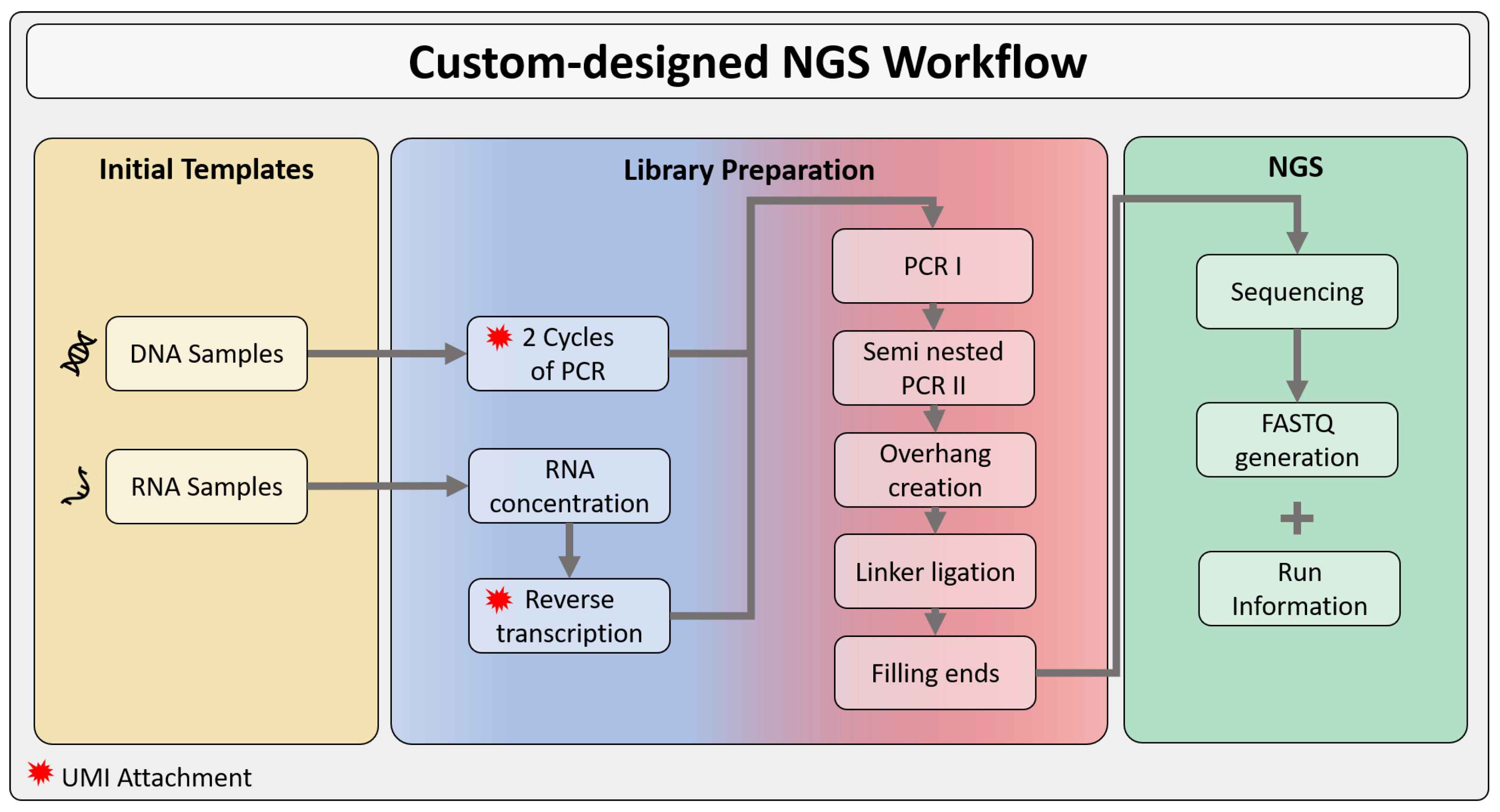
A custom-designed NGS workflow was developed to sequence RNA and DNA samples of the BCR::ABL1 fusion gene region (Figure 5—yellow). For both sample types UMIs were attached to each initial template (Figure 5—blue). For RNA samples, UMI attachment was performed during reverse transcription using UMI-containing gene-specific ABL1 primers and Superscript IV reverse transcriptase (Thermo Fisher Scientific, Waltham, MA, USA). UMI attachment to DNA controls (synthesized DNA that uses the RNA fusion transcript as a template sequence) was performed with two-cycle PCR using the same UMI-containing primer and Q5 polymerase (New England Biolabs, Ipswich, MA, USA). Fusion-gene selection was performed with a first PCR step using a forward primer in the BCR region and a reverse primer in the ABL1 region (see Table 3). In the course of library preparation, the region of interest, bearing most of the clinically relevant ABL1 mutations in CML cells including whole exons 4, 5, 6, and 7, was amplified in a second PCR with a single amplicon including the 10 bp-UMI attached to its 3’ end (Figure 5—red). In this study, the synthesized control DNA samples are used; CML patients’ samples are not considered.

3.1.1. Synthesized Control DNA Samples

IMPI’s methods are applied to synthesized BCR::ABL1 control DNA. This synthesized DNA was used for panel evaluation and determination of the LOD. To this end, a wt BCR::ABL1 control and three mutated BCR::ABL1 transcripts (p.E255K, p.T315I, and p.F359V) were synthesized (BioCat, Heidelberg, Germany). The mutated controls with clinically relevant resistance mutations were diluted with wt controls in different percentages for LOD evaluation: 5%, 1%, 0.5% VAF. For all samples, three replicates have been sequenced. To evaluate the extent of recombination events taking place during sample amplification, two mutated controls (100% p.E255K and 100% p.F359V) were mixed in equal parts before library preparation.

3.1.2. Next-Generation Sequencing

NGS (Figure 5—green) was performed on the Illumina MiSeq platform (Illumina, San Diego, CA, USA) using the V3 sequencing kit (600 cycles, 2 × 300 bp). This kit has the potential of sequencing 300 cycles per sequencing direction and enables a full sequencing coverage of the 586bp-region of interest with two largely non-overlapping reads.

3.1.3. Evaluation

The results of the UMI processing workflow implemented in IMPI were compared to the results of a standard NGS workflow (raw workflow). For all synthesized DNA controls, expected VAFs at specific loci are available. All synthesized DNA controls were analyzed for LOD evaluation.

3.2. Sample Pre-Processing

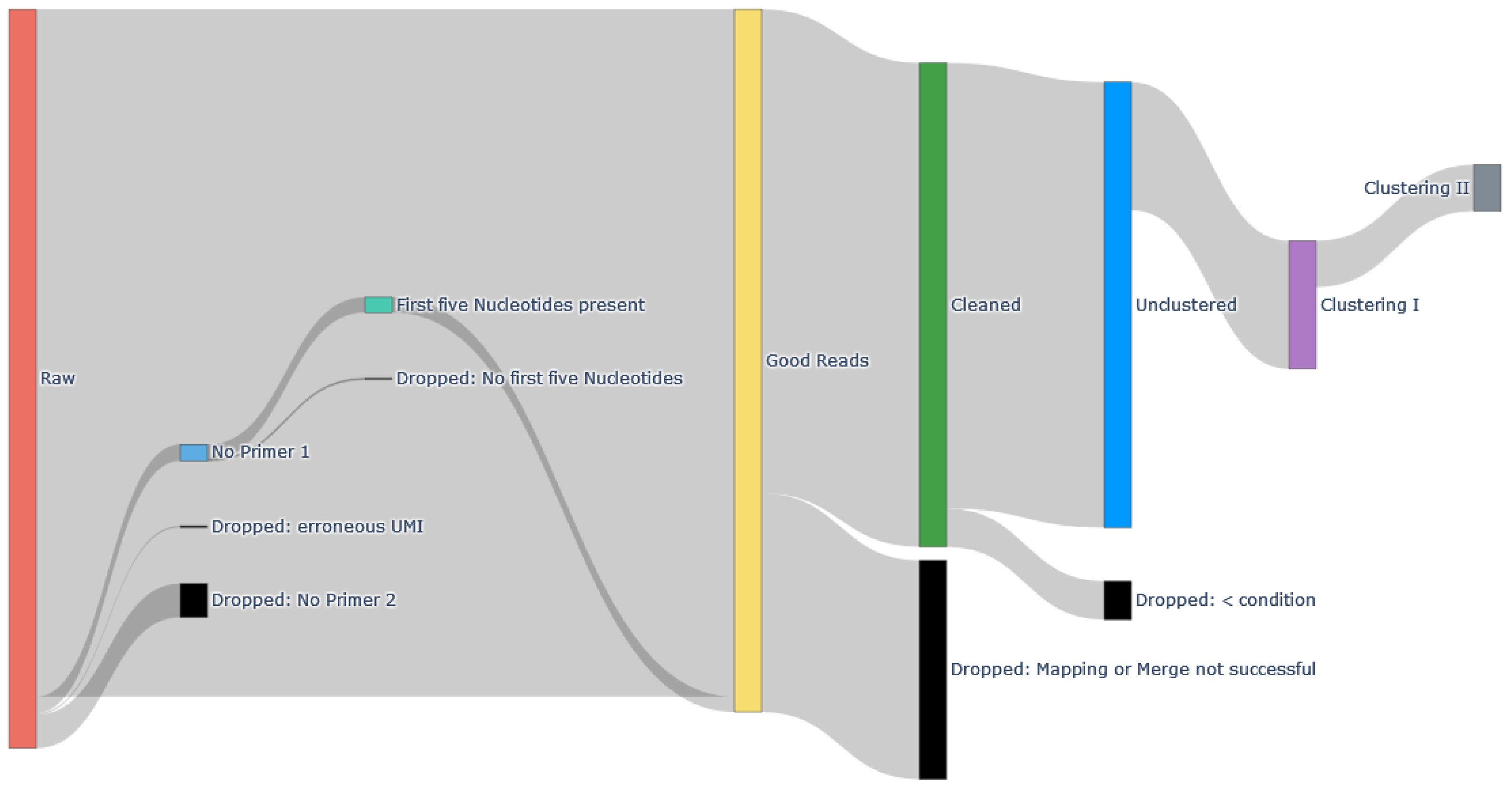
As described in Section 2.3, the IMPI workflow starts with the sample pre-processing (Figure 2). Thus, sample cleaning, UMI extraction, and feature calculations are carried out. Figure 6 shows the number of reads considered (colored) and not considered (black) for downstream analysis. As shown, in a first cleaning step, reads without reverse primer 2 (here: primer which contains UMI) and reads with aberrations within the length of the UMI are removed from the raw reads (red). Reads without a forward primer are not discarded if they contain the first five nucleotides according to the majority of all other reads. Reads which are not merged or mapped successfully are dropped as well. All reads are mapped on the BCR::ABL1 fusion gene reference sequence (transcript ID ENST00000318560). As shown, approximately one-third of the reads are dismissed after the first data cleaning step. The subsequent clustering steps further reduce the number of reads.

3.3. Cross-Sample Contamination

Once the pre-processing step is completed, the cross-sample contamination analysis can be applied to identify shared UMIs of two samples. As shown in Figure 7, IMPI provides on the left an interactive heatmap showing the number and percentage of shared UMIs. On the right, the overlap is visualized in a Venn diagram.

3.4. Raw Data, Clustering I, Clustering II

After the pre-processing step, IMPI allows clustering the reads according to their UMI. Here, IMPI implements two clustering methods which are described in Section 2.6. We evaluated and compared the results of these three different approaches applied to a wt sample (Figure 8A). The expected AF of the wt sequence (black line) is 100% at each locus, implying agreement with the reference sequence. All three replicates show a rather heterogeneous VAF in the 3’ end region of the reverse reads. Figure 8A further displays that the pre-processing and application of the clustering algorithms (Clustering I and Clustering II) implemented in IMPI show a lower variability within the results.
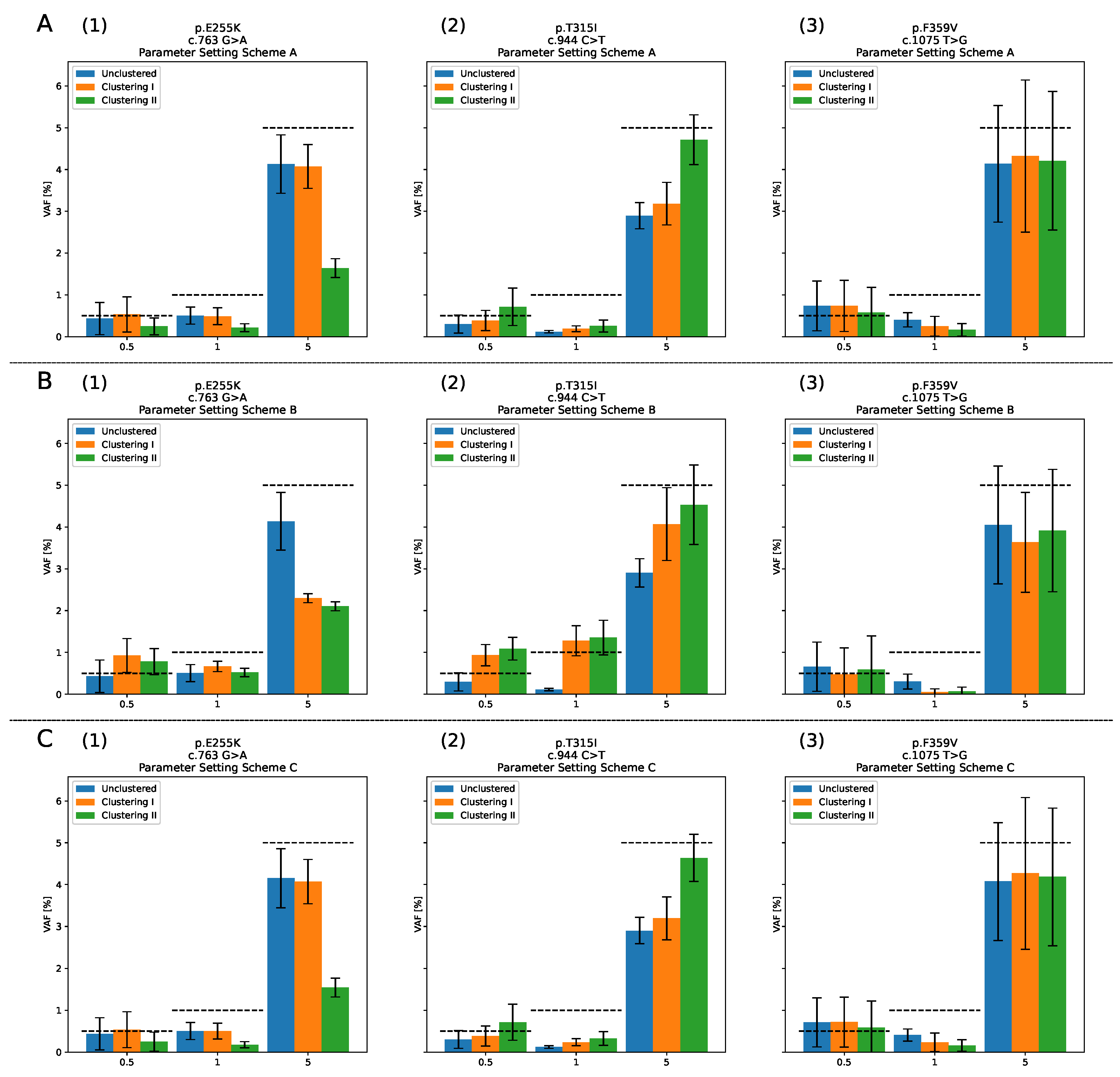
The results of the analysis of the three mentioned clinically relevant mutations in CML (p.E255K, p.T315I and p.F359V) are shown in Figure 9. Here, the subplots A–C show the average results of three replicates compared to the expected values (dashed lines) of the three implemented algorithms (blue: Unclustered, orange: Clustering I, and green: Clustering II) using three different parameter setting schemes. The parameter setting schemes are shown in Table 4, whereas parameter settings scheme A uses the default parameter setting of IMPI and scheme B is more restricted. Parameters defined in scheme C have been optimized by using the implemented evolution strategy. For the ES, one replicate of each mutated transcript of each concentration and one wt sample was used to determine the most suitable parameters.

4. Discussion

All methods implemented in IMPI have been applied to the provided NGS dataset consisting of synthesized BCR::ABL1 DNA samples. In comparison to other tools such as UMI-tools, UMICollapse, or zUMIs, IMPI provides a GUI (see Table 5). Further, IMPI executes automatically generated commands of third-party party tools (Bowtie2 and NGmerge). Additionally, the downloaded executables do not need any additional Python functionalities to be installed.
Here, IMPI is mainly compared with UMI-tools based on its functionalities. As described in Table 5, both, UMI-tools and IMPI are implemented in Python, use Bowtie2 for mapping but differ in the UMI collapsing and the GUI availability. The dataset served mainly for functionality demonstration and does not allow deep comparisons with UMI-tools results due to the datasets’ inherent limitations. These limitations, such as PCR-mediated recombination events and low sequencing depth, will be discussed in the later sections.

4.1. Data Cleaning

IMPI’s pre-processing methods prepare all data for further clustering, cross-sample contamination analysis, optimization steps, and export. In this step, methods are comparable to UMI-tools extract function and the required mapping steps using (as IMPI) Bowtie2. Further, UMI-tools requires SAMtools for conversion, sorting, and indexing. In this step, both tools check all reads for primers and extract the UMIs. As shown in Figure 6 and described in Section 3.2, in IMPI, approximately one-third of the reads are dismissed after the first data cleaning step. In this case, it is due to the used merging parameters (here: m i n i m u m o v e r l a p = 10 and allowed m i s m a t c h r a t e = 0.10 ).
For quality assurance, cross-sample contamination analysis has been performed. This method is especially helpful contamination is assumed, e.g., during wet lab sample processing. For example, in Figure 7, a subset of four samples is shown. When cross-sample contamination analysis has been performed for all 27 samples, no sample pair exceeded 4.87 % shared UMIs UMIs. This leads to the assumption that no cross-sample contamination occurred during sample processing.

4.2. Comparison: Raw Data, Clustering I and Clustering II

In the second step, clustering of the raw data by UMIs is performed. This method is comparable with UMI-tools’ dedup method, which is also used in UMICollapse after a different UMI clustering approach. As shown in Figure 8A and described in Section 3.4, wt VAF analysis shows an improvement by applying Clustering II. However, all three clustering processes show a rather heterogeneous VAF in the 3’ end region of the reverse reads. This region is known to offer a comparatively low average Phred quality score in all samples (shown in Figure 8B). Here, neither IMPI nor UMI-tools are able to successfully collapse UMIs to approach the expected 100%. Nevertheless, with the use of custom parameter settings and clustering algorithms, the results of Clustering II are closest to the expected results. The number of mutations (VAF > 0.5%) identified is reduced from 35 to 22. Results of UMI-tools show 36 identified mutations (VAF > 0.5%). These unsatisfactory results are not primarily related to the used tools – this is due to the sequencing strategy and is described in more detail in Section 4.3.
Looking closer into the results of the synthesized samples shown in Figure 9, the impact of minor parameter settings adaptations is visible. Individual parameter settings lead to different results. Allele frequencies of the p.F359V replicates show high variations (Figure 9A(3), B(3) and C(3)), which is very likely attributed to the low Phred quality score of the 3’ end region of the reverse read where this point-mutation is nearby. Conversely, point mutations further away from the overlapping read ends (p.E225K and p.T315I) show lower standard deviations than p.F359V.
All samples where parameter settings scheme B was applied (Figure 9B(1–3)) show in average better results in lower VAFs (0.5%)—especially, Clustering I and Clustering II. For higher expected mutation rates (1% and 5%) results show lower VAFs than results derived from parameter settings scheme A and C. As described in Table 4 (column B), parameter settings scheme B only uses clusters with at least two reads (Min. Clustersize  = 2 ). Consequently the number of reads for (V)AF calculation after clustering is reduced and calls much more variants. This means that an increased Min. Clustersize makes sense for samples with higher read counts.
When comparing the results of parameter settings scheme A and C, results look very similar but the ES optimizes parameter set allows more unspecific nucleotides (Max. N), insertions, and deletions. When comparing the average number of total point mutations detected (VAF > 0.5%), AF matrices generated by applying the optimized parameters of the ES show equal or less point mutations. Especially in the case of unclustered and Clustering I reads. For parameter settings scheme C, raw read analysis (unclustered) and results derived from Clustering I show an average number of point mutations (VAF > 0.5%) of 36.08 in unclustered and 37.71 in Clustering I. In Clustering II, in average 48.17 point mutations are detected.
The two clustering approaches perform differently. With our data, best results of the Clustering II are observed when being applied to p.T314I sample. For mutation detection in the beginning of the sequenced BCR::ABL1 gene Clustering II performed poorly. Near the read overlap region the three methods show similar results. However, it must be noted that the interpretation of these results is only partially possible because, as described in the next section, due to challenges while sequencing an exact interpretation of the results is not given.

4.3. LOD Evaluation

Highly sensitive NGS of synthesized positive controls revealed a position-dependent LOD. Using the UMI workflow, the LOD was 1% VAF for p.E255K, 5% VAF for p.T315I and 1% VAF for p.F359V. However, the raw workflow showed LOD of 1% VAF for p.E255K, 5% VAF for p.T315I and 5% VAF for p.F359V. In contrast to the literature [9], the use of UMIs does not show a significant increase in sensitivity in our workflow. Because of these unexpected LOD results, further experiments focusing on quantifying PCR-mediated recombination events during the library preparation were performed to find an explanation. These experiments revealed 12.25% recombination for positive controls after 30 cycles of PCR I. Here, PCR-mediated recombination causes a template switch of the polymerase during the elongation step of PCR [37]. In that affected 12.25% of the amplicons, a UMI, which initially tagged a mutated fragment, was transferred onto a wt read or vice versa. As a result, an initial template with a particular genotype and a corresponding UMI creates descendants showing sequences with other genetic information and other UMIs. This leads to conflicting base information in the collapse process if one amplicon represents a wt-base and another amplicon represents a variant base while both share the same UMI. The bioinformatics pipeline is set to call the base with the majority at a given position. Depending on the PCR cycle number of the recombination event, this can cause different base call results. Importantly, because of the single amplicon design of the workflow, those chimeric reads cannot be distinguished from correctly processed amplicons during mapping.
Subsequently, these contradictory results in UMI workflow evaluation of control samples can be attributed to PCR-mediated recombination. In standard NGS procedures, such PCR-mediated recombination events also happen, but they are not noticed since no backtracking to initial templates is usually done. One way to overcome this sensitivity problem is a basic workflow design change from a single amplicon sequencing approach to a multi amplicon sequencing approach. This change would decrease the probability of recombination events within the same amplicon. A further advantage of a multi-amplicon approach would be the possibility of sequencing with overlapping reads (a forward and a reverse read for the same amplicon), which would further improve sensitivity. Unfortunately, the long, non-overlapping reads of our design do not provide the ability to eliminate artifacts that arise due to sequencing strand bias.

5. Conclusions

To summarize, the ability to interpret the impact of UMIs in UMI-tagged NGS data shows high potential. As described within this study, comparing point mutation identification of raw reads versus reads collapsed by UMIs allows for data quality analysis as well as for better understanding of the data. Targeting this obstacles, IMPI was designed and developed. This software framework provides algorithms for NGS data pre- and processing, data quality assurance, handling UMI-tagged NGS data as well as providing compact and transparent results.
In this study, all algorithms implemented in IMPI were used to determine point mutations in BCR::ABL1 sequencing data derived from a custom-designed NGS approach. The use of UMIs for this sequencing data revealed no significant noise reduction compared to the raw workflow (without the use of UMIs). Comparing the results derived from IMPI’s raw read processing and clustering revealed discrepancies in VAFs. Consequently, experiments focusing on quantifying PCR-mediated recombination events during library preparation were carried out to find a reason for these discrepancies.
In conclusion, for this study, the implemented bioinformatics workflow, IMPI, could not eliminate all design and wet lab workflow limitations. However, the ability to compare raw data analysis and UMI clustering provided by IMPI made it possible to uncover these discrepancies. Other groups working with a similar sequencing concept were also unable to develop the design into a highly sensitive procedure [10]. This may indicate that future approaches should follow a modified strategy. Once wet lab experiments are improved, further development of the NGS workflow design towards smaller amplicons could exploit the power of the here described bioinformatics pipeline and thus the potential of highly sensitive sequencing. Finally, the current advances in artificial intelligence and the upcoming possibilities can not be ignored in the field of genomics and variant detection. With the integration of an evolution strategy into IMPI, the first attempt has been performed and opens up chances for further improvement.

Author Contributions

Conceptualization, J.V., J.B., S.M.W. and S.S.; Methodology, J.V. and J.B.; Software, J.V.; Validation, J.V. and J.B.; Formal Analysis, J.V. and J.B.; Investigation, J.B., T.M. and G.W.; Resources, J.B., T.M. and G.W.; Data Curation, J.V. and J.B.; Writing—Original Draft Preparation, J.V. and J.B.; Writing—Review & Editing, A.M.L., T.M., G.W., M.W., S.M.W. and S.S.; Visualization, J.V.; Supervision, G.W., M.W., S.M.W. and S.S.; Project Administration, S.M.W. and S.S.; Funding Acquisition, J.V. and S.M.W. All authors have read and agreed to the published version of the manuscript.

Funding

This work has been funded by the Austrian Research Promotion Agency (FFG), the dissertation program of the FH OOE (funded by Land OOE), FH OOE’s Center of Technical Innovation in Medicine (TIMed) and Incyte Inc. The funding body had no influence on design of the software or design, collection, analysis and interpretation of data or writing the manuscript.

Institutional Review Board Statement

Not applicable.

Informed Consent Statement

Not applicable.

Data Availability Statement

The most recent version of the IMPI software, its documentation, and a test data subset is available here: https://bioinformatics.fh-hagenberg.at/pointmutationdetector/ (accessed on 28 March 2024).

Conflicts of Interest

The authors declare that they have no competing interests.

Abbreviations

The following abbreviations are used in this manuscript:
ABL1Abelson murine leukemia viral oncogene homolog 1
AFAllele frequency
ATPAdenosine triphosphate
BCRBreakpoint cluster region
BWABurrows-Wheeler Aligner
CIGARConcise Idiosyncratic Gapped Alignment Report
CMLChronic myeloid leukemia
ESEvolution strategy
GATKGenome Analysis Toolkit
GUIGraphical user interface
IMPIInterface for Point Mutation Identification
LODLimit of detection
MSEMean squared error
NGSNext-generation sequencing
OSOperating system
PCRPolymerase chain reaction
PWMPosition weight matrix
SAMSequence alignment map
TKITyrosine kinase inhibitors
UMIUnique molecular identifier
VAFVariant allele frequency
wtWild-type

References

  1. Cibulskis, K.; Lawrence, M.S.; Carter, S.L.; Sivachenko, A.; Jaffe, D.; Sougnez, C.; Gabriel, S.; Meyerson, M.; Lander, E.S.; Getz, G. Sensitive detection of somatic point mutations in impure and heterogeneous cancer samples. Nat. Biotechnol. 2013, 31, 213–219. [Google Scholar] [CrossRef]
  2. Lin, M.T.; Mosier, S.L.; Thiess, M.; Beierl, K.F.; Debeljak, M.; Tseng, L.H.; Chen, G.; Yegnasubramanian, S.; Ho, H.; Cope, L.; et al. Clinical validation of KRAS, BRAF, and EGFR mutation detection using next-generation sequencing. Am. J. Clin. Pathol. 2014, 141, 856–866. [Google Scholar] [CrossRef]
  3. Tsiatis, A.C.; Norris-Kirby, A.; Rich, R.G.; Hafez, M.J.; Gocke, C.D.; Eshleman, J.R.; Murphy, K.M. Comparison of Sanger sequencing, pyrosequencing, and melting curve analysis for the detection of KRAS mutations: Diagnostic and clinical implications. J. Mol. Diagn. 2010, 12, 425–432. [Google Scholar] [CrossRef]
  4. Schmitt, M.W.; Pritchard, J.R.; Leighow, S.M.; Aminov, B.I.; Beppu, L.; Kim, D.S.; Hodgson, J.G.; Rivera, V.M.; Loeb, L.A.; Radich, J.P. Single-molecule sequencing reveals patterns of preexisting drug resistance that suggest treatment strategies in Philadelphia-positive leukemias. Clin. Cancer Res. 2018, 24, 5321–5334. [Google Scholar] [CrossRef]
  5. Alikian, M.; Gerrard, G.; Subramanian, P.G.; Mudge, K.; Foskett, P.; Khorashad, J.S.; Lim, A.C.; Marin, D.; Milojkovic, D.; Reid, A.; et al. BCR-ABL1 kinase domain mutations: Methodology and clinical evaluation. Am. J. Hematol. 2012, 87, 298–304. [Google Scholar] [CrossRef]
  6. Potapov, V.; Ong, J.L. Examining Sources of Error in PCR by Single-Molecule Sequencing. PLoS ONE 2017, 12, e0169774. [Google Scholar] [CrossRef]
  7. Smith, T.; Heger, A.; Sudbery, I. UMI-tools: Modeling sequencing errors in Unique Molecular Identifiers to improve quantification accuracy. Genome Res. 2017, 27, 491–499. [Google Scholar] [CrossRef]
  8. Mansukhani, S.; Barber, L.J.; Kleftogiannis, D.; Moorcraft, S.Y.; Davidson, M.; Woolston, A.; Proszek, P.Z.; Griffiths, B.; Fenwick, K.; Herman, B.; et al. Ultra-sensitive mutation detection and genome-wide DNA copy number reconstruction by error-corrected circulating tumor DNA sequencing. Clin. Chem. 2018, 64, 1626–1635. [Google Scholar] [CrossRef]
  9. Boltz, V.F.; Rausch, J.; Shao, W.; Hattori, J.; Luke, B.; Maldarelli, F.; Mellors, J.W.; Kearney, M.F.; Coffin, J.M. Ultrasensitive single-genome sequencing: Accurate, targeted, next generation sequencing of HIV-1 RNA. Retrovirology 2016, 13, 87. [Google Scholar] [CrossRef] [PubMed]
  10. Parker, W.T.; Phillis, S.R.; Yeung, D.T.; Lawrence, D.; Schreiber, A.; Wang, P.; Geoghegan, J.; Lustgarten, S.; Hodgson, G.; Rivera, V.M.; et al. Detection of BCR-ABL1 Compound and Polyclonal Mutants in Chronic Myeloid Leukemia Patients Using a Novel Next Generation Sequencing Approach That Minimises PCR and Sequencing Errors. Blood 2014, 124, 399. [Google Scholar] [CrossRef]
  11. Langmead, B.; Salzberg, S.L. Fast gapped-read alignment with Bowtie 2. Nat. Methods 2012, 9, 357–359. [Google Scholar] [CrossRef]
  12. Li, H.; Durbin, R. Fast and accurate short read alignment with Burrows–Wheeler transform. Bioinformatics 2009, 25, 1754–1760. [Google Scholar] [CrossRef]
  13. Bray, N.L.; Pimentel, H.; Melsted, P.; Pachter, L. Near-optimal probabilistic RNA-seq quantification. Nat. Biotechnol. 2016, 34, 525–527. [Google Scholar] [CrossRef]
  14. Svensson, V.; Natarajan, K.N.; Ly, L.H.; Miragaia, R.J.; Labalette, C.; Macaulay, I.C.; Cvejic, A.; Teichmann, S.A. Power analysis of single-cell RNA-sequencing experiments. Nat. Methods 2017, 14, 381–387. [Google Scholar] [CrossRef]
  15. Liu, D. Algorithms for efficiently collapsing reads with Unique Molecular Identifiers. PeerJ 2019, 7, e8275. [Google Scholar] [CrossRef]
  16. Parekh, S.; Ziegenhain, C.; Vieth, B.; Enard, W.; Hellmann, I. zUMIs-a fast and flexible pipeline to process RNA sequencing data with UMIs. Gigascience 2018, 7, giy059. [Google Scholar] [CrossRef]
  17. Xia, X. Position weight matrix, gibbs sampler, and the associated significance tests in motif characterization and prediction. Scientifica 2012, 2012, 917540. [Google Scholar] [CrossRef]
  18. Beyer, H.G.; Schwefel, H.P. Evolution strategies: A comprehensive introduction. Nat. Comput. 2002, 1, 3–52. [Google Scholar] [CrossRef]
  19. Gaspar, J.M. NGmerge: Merging paired-end reads via novel empirically-derived models of sequencing errors. BMC Bioinform. 2018, 19, 536. [Google Scholar] [CrossRef] [PubMed]
  20. Li, H.; Handsaker, B.; Wysoker, A.; Fennell, T.; Ruan, J.; Homer, N.; Marth, G.; Abecasis, G.; Durbin, R. The Sequence Alignment/Map format and SAMtools. Bioinformatics 2009, 25, 2078–2079. [Google Scholar] [CrossRef] [PubMed]
  21. Koboldt, D.C.; Zhang, Q.; Larson, D.E.; Shen, D.; McLellan, M.D.; Lin, L.; Miller, C.A.; Mardis, E.R.; Ding, L.; Wilson, R.K. VarScan 2: Somatic mutation and copy number alteration discovery in cancer by exome sequencing. Genome Res. 2012, 22, 568–576. [Google Scholar] [CrossRef] [PubMed]
  22. Van der Auwera, G.A.; O’Connor, B.D. Genomics in the Cloud: Using Docker, GATK, and WDL in Terra; O’Reilly Media: Sebastopol, CA, USA, 2020. [Google Scholar]
  23. Poplin, R.; Ruano-Rubio, V.; DePristo, M.A.; Fennell, T.J.; Carneiro, M.O.; Van der Auwera, G.A.; Kling, D.E.; Gauthier, L.D.; Levy-Moonshine, A.; Roazen, D.; et al. Scaling accurate genetic variant discovery to tens of thousands of samples. BioRxiv 2017, 201178. [Google Scholar]
  24. Xia, L.; Li, Z.; Zhou, B.; Tian, G.; Zeng, L.; Dai, H.; Li, X.; Liu, C.; Lu, S.; Xu, F.; et al. Statistical analysis of mutant allele frequency level of circulating cell-free DNA and blood cells in healthy individuals. Sci. Rep. 2017, 7, 7526. [Google Scholar] [CrossRef] [PubMed]
  25. Singh, P. Learn Windows Subsystem for Linux; Apress: Berkley, CA, USA, 2020; pp. 1–17. [Google Scholar]
  26. Simon, J.S.; Botero, S.; Simon, S.M. Sequencing the peripheral blood B and T cell repertoire—Quantifying robustness and limitations. J. Immunol. Methods 2018, 463, 137–147. [Google Scholar] [CrossRef] [PubMed]
  27. Tretyakov, K. Matplotlib-Venn: Functions for Plotting Area-Proportional Two-and Three-Way Venn Diagrams in Matplotlib. 2020. Available online: https://pypi.org/project/matplotlib-venn/ (accessed on 28 March 2024).
  28. Kang, Z.J.; Liu, Y.F.; Xu, L.Z.; Long, Z.J.; Huang, D.; Yang, Y.; Liu, B.; Feng, J.X.; Pan, Y.J.; Yan, J.S.; et al. The Philadelphia chromosome in leukemogenesis. Chin. J. Cancer 2016, 35, 48. [Google Scholar] [CrossRef] [PubMed]
  29. Rumpold, H.; Webersinke, G. Molecular pathogenesis of Philadelphia-positive chronic myeloid leukemia—Is it all BCR-ABL? Curr. Cancer Drug Targets 2011, 11, 3–19. [Google Scholar] [CrossRef] [PubMed]
  30. Reddy, E.P.; Aggarwal, A.K. The ins and outs of bcr-abl inhibition. Genes Cancer 2012, 3, 447–454. [Google Scholar] [CrossRef] [PubMed]
  31. Druker, B.J. Translation of the Philadelphia chromosome into therapy for CML. Blood 2008, 112, 4808–4817. [Google Scholar] [CrossRef] [PubMed]
  32. Jabbour, E.; Kantarjian, H. Chronic myeloid leukemia: 2020 update on diagnosis, therapy and monitoring. Am. J. Hematol. 2020, 95, 691–709. [Google Scholar] [CrossRef]
  33. Ramirez, P.; DiPersio, J.F. Therapy options in imatinib failures. Oncologist 2008, 13, 424–434. [Google Scholar] [CrossRef]
  34. Chopade, P.; Akard, L.P. Improving Outcomes in Chronic Myeloid Leukemia Over Time in the Era of Tyrosine Kinase Inhibitors. Clin. Lymphoma Myeloma Leuk. 2018, 18, 710–723. [Google Scholar] [CrossRef]
  35. Braun, T.P.; Eide, C.A.; Druker, B.J. Response and resistance to BCR-ABL1-targeted therapies. Cancer Cell 2020, 37, 530–542. [Google Scholar] [CrossRef]
  36. Andrews, S. FastQC: A Quality Control Tool for High throughput Sequence Data. 2010. Available online: https://www.bioinformatics.babraham.ac.uk/projects/fastqc/ (accessed on 28 March 2024).
  37. Shao, W.; Boltz, V.F.; Spindler, J.E.; Kearney, M.F.; Maldarelli, F.; Mellors, J.W.; Stewart, C.; Volfovsky, N.; Levitsky, A.; Stephens, R.M.; et al. Analysis of 454 sequencing error rate, error sources, and artifact recombination for detection of Low-frequency drug resistance mutations in HIV-1 DNA. Retrovirology 2013, 10, 18. [Google Scholar] [CrossRef] [PubMed]
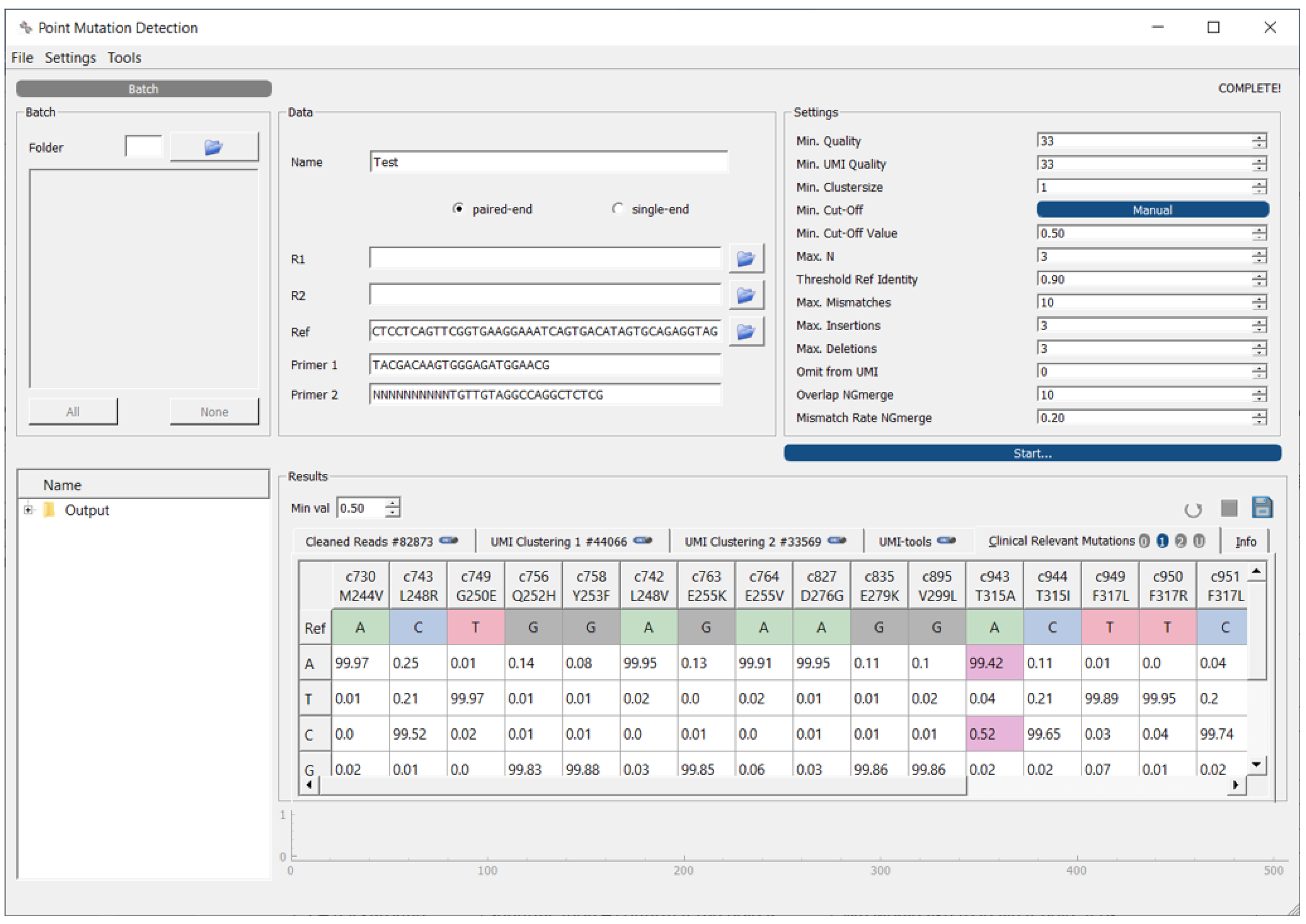
Figure 1. Screenshot of the IMPI GUI.
Biomedinformatics 04 00071 g001
Figure 2. Representation of the IMPI workflow starting with the input setup (yellow) which includes raw data pre-processing and is followed by the data analysis step (blue) that comprise all algorithms for clustering and raw data evaluation. Finally, IMPI outputs are generated (green). Additionally, IMPI provides three optimization methods (red): Cross-sample contamination analysis based on shared UMIs in multiple samples, an evolution strategy for settings parameter optimization, and a wild-type (wt) correction method.
Biomedinformatics 04 00071 g002
Figure 3. Clustering of reads by UMIs. Unique UMIs are collapsed in a first step (Clustering I) and re-clustered, allowing mismatches (Clustering II). For each cluster, consensus sequences are built.
Biomedinformatics 04 00071 g003
Figure 4. Graphical representation of parameter optimization using an evolution strategy in IMPI. Multiple files with known VAFs can be used to find the best parameters for a given dataset. The implemented evolution strategy provides fitting parameter settings based on these files and expected allele frequencies at specific loci. Additionally, IMPI indicates if all required files are available (green) or not (red).
Biomedinformatics 04 00071 g004
Figure 5. Custom-designed NGS Workflow. Starting material was either DNA or RNA samples (yellow). Sample pre-processing (blue) differs in the method of UMI attachment. UMI attachment in DNA samples was performed by using a two-cycle PCR; UMI attachment in RNA samples was completed during reverse transcription. Library preparation (red) was the same for both sample types. The region of interest (including the UMIs) was selectively amplified using two steps of PCR followed by linker ligation necessary for Illumina sequencing. Finally, after NGS, FASTQ files were generated and run information was provided for further processing (green).
Biomedinformatics 04 00071 g005
Figure 6. Sankey diagram showing the number of reads within the pre-processing and clustering steps. Different exclusion criteria at different steps were implemented: (1) reverse read does not contain a primer (here: Primer 2), (2) reads containing erroneous forward primers without first five nucleotides, (3) unsuccessfully merged reads, (4) reads that do not fulfill the conditions according to the set parameters (see Table 2).
Biomedinformatics 04 00071 g006
Figure 7. Screenshot of IMPI’s cross-sample contamination analysis. Left: a heatmap inclusing four different samples showing the percentage and number (#) of shared UMIs between two samples. Right: a Venn diagram of two samples (E225K1II_34 in blue and T315I1II_S42 in green), which share 2171 UMIs (=2.88%).
Biomedinformatics 04 00071 g007
Figure 8. Results provided by IMPI for a wild-type sample. (A) Allele frequencies (AFs) of a wild-type (wt) sample where AFs are expected to be 100% and identical to the reference sequence. Results show an average allele frequency of 99.80% with a maximum aberration of 2.72% (unclustered) and 7.76% (UMI-tools). Clustering I and II slightly improve the AF ratios and reduce the number of detected point mutations (VAFs > 0.5%) from 35 to 22. UMI-tools results, shown in green, show similar results with 36 detected point mutations (VAFs > 0.5%). Low AFs (<99.5%) in the region of the 3’ end of the reverse read highly agree with the low qualities of the reverse reads shown in (B)—graphs have been generated using FastQC [36]. The implemented variant calling algorithm in IMPI compensates for more extreme deviations.
Biomedinformatics 04 00071 g008
Figure 9. Comparison of the three algorithms for variant allele frequency calculation (Unclustered, Clustering I, and Clustering II). (AC) show the mean VAFs of the synthesized control samples with the different clinically relevant mutations (p.E255K, p.T315I and p.F359V). Dashed lines show the expected VAFs. For the different parameter setting schemes described in Table 4 A–C the measured results are shown. We show that minor parameter alterations (Scheme A to Scheme B) lead to improved results, especially in p.E255K 0.5% expected VAF. Results mainly differ in 1% expected VAF. However, in all samples in scheme A between 14 (Clustering II) and 44 (Unclustered) point mutations (VAF > 0.5%) and in (Scheme B) between 12 (Clustering II) and 38 (Clustering I) point mutations are detected. (C) Parameters have been optimized using the implemented ES in IMPI and were applied to synthesized mutated transcripts with 0.5%, 1%, and 5% VAF. For all schemes sample t-tests have been performed. No statistically significant differences were detected, except in the following: A1-C1 5% VAF Clustering II (green), B1 5% VAF Clustering I (orange), A2-B2 1% and 5% VAF unclustered (blue), A3-C3 1% VAF unclustered (blue) and both clustering approaches (orange and green).
Biomedinformatics 04 00071 g009
Table 1. Features extracted and processed from the SAM output file derived from Bowtie2 mapping.
Feature NameDescription
IDRead identifier extracted from the FASTQ file source
UMIExtracted unique molecular identifier sequence which was part of the primer
UMI_Phred_QualityPhred quality scores of the UMI encoded in ASCII characters
UMI_Avg_ScoreAverage Phred quality score of the UMI
SeqNucleotide sequence of the read with its deletions and insertions which are defined by the Concise Idiosyncratic Gapped Alignment Report (CIGAR) [20] information
Phred_QualityPhred quality scores of the whole nucleotide sequence encoded in ASCII characters
Avg_ScoreAverage Phred quality score of the sequence
StartStart position of the sequence within the reference gene sequence
LengthLength of the sequence
InsertionsNumber of insertions
DeletionsNumber of deletions
RefIdenticalIdentity of the sequence with the reference gene sequence
RefMismatchesNumber of mismatches in comparison with the reference gene sequence
aaSeqTranslated nucleotide sequence to get the amino acid sequence
aaRefIdenticalIdentity of the amino acid sequence with the amino acid reference sequence
aaRefMismatchesNumber of mismatches in comparison with the amino acid reference sequence
Table 2. Adjustable parameters for calculating allele frequency matrices.
Parameter NameDescription
Min. QualityAll sequences with a lower average Phred quality score are excluded for calculating the AF matrices
Min. UMI QualityAll sequences with a lower average Phred quality score of the UMI are excluded
Min. ClustersizeWhen clustering algorithms are applied, all clusters with a size lower than requested are discarded
Min. Cut-Off and Min. Cut-Off ValueThe minimal cut-off value defines the rate of identical nucleotides of the reads within one cluster to be identical and confirm this nucleotide—if Min. Cut-Off is set Dynamic, the cut-off value depends on the cluster size—the larger the cluster, the higher the need of identical bases for defining a nucleotide at a specific gene location
Max. NWhen a nucleotide at a specific position is not confirmed and is defined as N—this value defines the maximum N per sequence
Threshold Ref IdentityOnly sequences with a reference gene correspondence are taken for AF matrix calculation
Max. Mismatches, Max. Insertions and Max. DeletionsDefinition of the maximal number of mismatches, insertions or deletions
Omit from UMISince the first few nucleotides within a read show rather low quality IMPI allows for omitting nucleotides from the UMI
Overlap NGmergeDefines the number of nucleotides that are allowed to overlap when using NGmerge (only relevant in pre-processing step)
Mismatch Rate NGmergeDefines the maximum rate of mismatches when in overlapping regions
Table 3. Primer used in the custom-designed NGS workflow. The BCR::ABL1 fusion-gene selection was performed using a forward primer in the BCR region and a UMI-containing reverse primer in the ABL1 region.
 Primer Sequence
ForwardTACGACAAGTGGGAGATGGAACG
ReverseNNNNNNNNNNTGTTGTAGGCCAGGCTCTCG
Table 4. Parameter setting schemes used for point mutation identification. Parameter setting scheme C is the optimized parameter scheme identified by the ES implemented in IMPI.
ABC
Min. Quality333534
Min. UMI Quality333431
Min. Clustersize121
Min. Cut-Off and Min. Cut-Off Value0.500.500.50
Max. N31011
Threshold Ref Identity0.900.950.94
Max. Mismatches10511
Max. Insertions3120
Max. Deletions3120
Omit from UMI000
Table 5. Tools for dealing with UMIs.
MappingOperating SystemGUI/Command-Line-BasedImplementation
UMI-tools [7]Bowtie2, e.g.,LinuxcmdPython
zUMIs [16]STARLinuxcmdR
UMICollapse [15]Bowtie2 *, e.g.,LinuxcmdJava
umis [14]Kallisto/RapMap **Windows, LinuxcmdPython
IMPIBowtie2Windows, LinuxGUI + cmdPython
* uses UMI-tools dedup method in second step; ** pseudo-aligners.
Disclaimer/Publisher’s Note: The statements, opinions and data contained in all publications are solely those of the individual author(s) and contributor(s) and not of MDPI and/or the editor(s). MDPI and/or the editor(s) disclaim responsibility for any injury to people or property resulting from any ideas, methods, instructions or products referred to in the content.