Simulation-Based Investigation of On-Demand Vehicle Deployment for Night Bus Routes Using the Monte Carlo Method

Abstract

Public transportation systems, including trams and buses, play a crucial role in urban traffic. However, these traditional modes of transport have some well-known drawbacks, such as long distances between stops, lengthy waiting times, and a lack of privacy. In response to these challenges, an innovative mobility concept called “FLAIT-train” offers potential solutions. The FLAIT-train operates on regular roads and aims to provide DOOR-2-DOOR transport, addressing the issues associated with fixed stops and offering increased accessibility and convenience. In its initial phase, the FLAIT-train operates on exclusive lanes, but it is designed to integrate with other traffic eventually. The vehicle technology of FLAIT-trains closely resembles that of battery electric autonomous vehicles. To assess whether FLAIT-trains can be used as a suitable alternative to conventional public transportation systems, this paper employs traffic simulations that consider key performance indicators, including the average waiting time per passenger, maximum waiting time of a single passenger, average in-vehicle time per passenger, and average occupancy rate of the vehicles. Using SUMO software (“Simulation of Urban Mobility”, version 1.12.0), a night bus service scenario is meticulously designed and generated. Within this scenario, both FLAIT-trains and conventional buses are simulated under identical conditions and based on statistical data.

1. Introduction

Tram and bus systems offer valuable economic and environmental advantages as essential elements of public transportation, contributing to improved sustainability and urban living standards [1]. Nevertheless, they face specific challenges that can affect their acceptance and usage.

Poor accessibility to fixed stops is a significant issue affecting the attractiveness of trams or buses [2], especially during the night when there are fewer active night bus routes, such as in the German city Duisburg. Passengers often find themselves having to walk long distances to reach a stop, and in some cases, they may even have to cross several streets to access the nearest stop. This inconvenience can deter potential passengers and reduce the overall appeal of using public transportation.

Optimizing the total travel time is another crucial aspect to consider for public modes of transport, such as buses. The total travel time includes various components, including the time to walk to and from the boarding and alighting stops, the waiting time at the stop, and the actual in-vehicle travel time.

Another area for improvement is the in-vehicle time, which can be optimized by minimizing the number of intermediate stops and reducing the boarding and alighting times.

Furthermore, ensuring passenger privacy and comfort is indeed an important aspect of public transportation. Trams or buses, being shared public spaces, can sometimes lack the level of privacy that individual travelers might prefer. Passengers may feel uncomfortable due to the proximity of fellow passengers, especially during rush hours when trams or buses are crowded [3].

Conversations between passengers, phone calls, and other activities can contribute to a sense of reduced privacy for some passengers. This can be challenging, especially for those seeking a quieter and more private environment during their commute.

Additionally, as demonstrated by studies such as [4], the limited number of seats in trams or buses can be a concern for passengers, leading to discomfort during long journeys. Standing for extended periods may also impact passenger satisfaction. Furthermore, an inadequate air quality, especially during rush hours when trams or buses are packed with passengers, can add to the perceived discomfort [3].

A night bus service presents a unique application scenario for public transportation, as the number of passengers is usually much lower at night. The reduced passenger volume results in longer intervals between two consecutive night buses, e.g., departing only once every hour in the German city Duisburg. The fixed schedule restricts passengers from returning home at their preferred time, and they must plan their travel around the scheduled departure time.

However, innovative, on-demand transportation concepts, like the DOOR-2-DOOR service [5], have gained attention as potential solutions to overcome the limitations of conventional public transportation systems. The DOOR-2-DOOR service aims to provide a more flexible and personalized transport option for passengers, offering them a convenient and efficient way to travel from their doorstep to their destination without the need to adhere to fixed schedules or stops.

Since 2019, an innovative concept called “Fast Lane AI Transportation” (FLAIT) has been under development [6]. The ultimate goal of this research is to achieve an on-demand DOOR-2-DOOR service using a single FLAIT vehicle. However, due to current technological limitations, this goal needs to be pursued incrementally. This paper presents an intermediate solution aimed at addressing the challenges faces by conventional public transportation systems. Building on ongoing research regarding modular buses [7], the FLAIT-trains, comprised of FLAIT vehicles, have the potential to replace traditional public transportation systems. If the application of such systems can enhance the attractiveness of the public transportation system, it will increase the utilization rate of public transportation compared to private cars. As a result, some advantages of the public transportation system, such as the efficient use of urban spaces, would be significantly improved.

This paper focuses on exploring the feasibility and performance of the FLAIT-train system as a potential replacement for conventional public transportation. Through a simulative analysis, the research is aimed to assess the effectiveness of this alternative transportation approach in the context of a night bus scenario.

2. Related Work

The study of on-demand transport systems includes research on the Dial-a-Ride Problem (DARP). The DARP involves transporting passengers between paired pickup (origin) and delivery points (destination) and has been a subject of study for over five decades [8,9].

Dial-a-Ride services can be provided in either a static or a dynamic mode, as described by [10]. In a static mode, all transportation requests are known in advance, allowing for preplanned routes and schedules. On the other hand, in the dynamic mode, transportation requests are revealed in real time, and vehicle routes are adjusted accordingly [10,11]. The dynamic mode allows for more flexibility and adaptability to changing demands.

Dial-a-Ride Problems (DARPs) can be classified into two main categories: single-vehicle DARPs (SDARPs) and multi-vehicle DARPs. These categories are based on the number of vehicles involved in transporting passengers, as described by [10].

In the single-vehicle DARP (SDARP) scenario, all passengers are served and transported by a single vehicle. This represents the simplest and most straightforward case of the DARP. The SDARP can be seen as a basic variant of the problem, where the goal is to find the most efficient routes for a single vehicle to serve all the pickup and delivery requests.

On the other hand, the multi-vehicle DARP involves multiple vehicles to serve the passengers’ transportation needs. In this case, the optimization challenge becomes more complex, as the routes for multiple vehicles need to be planned to ensure an efficient and timely service for all passengers.

Indeed, Personal Rapid Transit (PRT) is another alternative on-demand transport system that has been extensively researched and studied, as stated in [12,13].

PRT is an automated transit system that operates with driverless vehicles. It consists of a fixed network with dedicated off-line stops. One of the key advantages of the PRT system is its smaller vehicle size, typically accommodating 2 to 4 passengers. Due to its on-demand technology, the PRT system can provide faster travel times by avoiding intermediate stops, offering passengers a more direct and efficient transportation experience [12].

One of the significant differences between the PRT system and other transportation systems is that PRT traffic does not interfere with other traffic participants. This is achieved by elevating the PRT track to a higher level or concealing it underground, effectively separating it from pedestrian and vehicular traffic. As a result, the PRT system can ensure a high level of safety and efficiency in its operation [13].

However, it is essential to note that the PRT system comes with considerable investment costs for its infrastructure. According to research in [12], the investment costs for PRT tracks can range from USD 30 to 100 million per mile due to the exclusivity and technical complexity of the system.

While the PRT system offers several advantages in terms of safety, efficiency, and direct travel, its high infrastructure costs may present a challenge to its widespread implementation. Nonetheless, the PRT and DARP services present promising alternatives in the field of on-demand transport systems, each with unique features and capabilities that cater to different transportation needs.

2.1. Scientific Research of the DARP

Since the introduction of the first Dial-a-Ride Problem (DARP) service in 1970, a substantial amount of research has focused on developing models and algorithms to address its various aspects. Notably, the research progress up to 2007 was thoroughly summarized and described in [14]. The publication provided a comprehensive overview of the advancements made in the DARP field up until that time.

In more recent years, from 2008 to 2018, further research and developments in the DARP domain were documented and presented in [9]. This study showcased the latest findings and methodologies in handling the DARP, reflecting the ongoing efforts to improve and optimize this on-demand transportation system.

Furthermore, an update on the research progress in the DARP domain up until 2021 was provided in [15]. This publication compiled and summarized the relevant works and contributions made in the DARP field during the years leading up to 2021, shedding light on the latest findings and innovations in the domain.

The pioneering work on planning and scheduling for the Dial-a-Ride Problem (DARP) was presented in [16]. Subsequently, research in this area has been continuously studied for different cases and scenarios. As highlighted in the research in [14], the publications on the DARP have primarily focused on two main problem objectives:

• Minimizing costs while ensuring full demand satisfaction and adhering to various side constraints;
• Maximizing the number of satisfied demand requests, taking into account vehicle availability and other side constraints.

These side constraints often include factors such as the fleet size, operational costs, and driver’s wages. The common goal is to find solutions that optimize the overall efficiency and effectiveness of the DARP system. Satisfied demand refers to meeting customer preferences and requirements, such as minimizing the waiting time, in-vehicle time, or the total duration of the route.

In 1980, ref. [17] analyzed and solved the single-vehicle case of the DARP in static mode using a dynamic program. The objective was to minimize a combined objective function comprising the route duration, total waiting time, and in-vehicle time for all passengers. Concurrently, other researchers also explored this problem using Benders’ decomposition procedure [18,19].

Subsequent research on single-vehicle DARPs employed various approaches. In one study, the DARP was formulated as a k-forest problem to optimize the total routing distance [20]. Another investigation [21] aimed to optimize the cost effectiveness of a single-vehicle DARP and the total travel distance using metaheuristic techniques, such as simulated annealing, generic algorithms, particle swarm optimization, and artificial immune system.

Since the research conducted in [22], most publications have primarily focused on developing multi-vehicle DARPs, each distinguished by varying constraints and objective functions. Some studies aimed to minimize the travel costs, including the total ride distance and duration, assuming an efficient number of available vehicles [10,23,24,25]. On the other hand, some researchers sought to maximize the service quality measures with a limited number of available vehicles [26,27,28].

Moreover, some publications also considered the vehicle emissions as an additional factor in the optimization process [29]. Other objective functions included the passenger occupancy rate [30], service provider’s operational costs and profit [31,32,33], workforce planning and staff workload [34], and system reliability [35].

Interested readers can refer to the detailed introductions and classifications available in [5,10,11] for a more comprehensive understanding of the different models and algorithms. These works provide valuable insights into the various approaches taken to tackle the multifaceted challenges presented by multi-vehicle DARPs.

2.2. Application Projects of the DARP in Germany

In North and South America and Asia, ride-hailing services have gained immense popularity as on-demand mobility solutions, with transportation network companies like Uber, Lyft, and DiDi dominating the market. However, in Germany, these ride-hailing services are not as common due to strict regulations [36]. Instead, the country has seen the emergence of on-demand mobility services in the form of ride pooling. Several private enterprises or startups have ventured into this space, such as MOIA, which has been operating in Hamburg and Hannover since 2019 and 2017, respectively [36].

Furthermore, collaborations between municipal transportation companies and startups have led to the establishment of additional on-demand mobility services. For instance, LüMo operates in Lübeck, myBus in Duisburg, and SSB Flex in Stuttgart [37]. A notable example is the “Bedarfsbus Schorndorf” service, which operates as part of a research project [38].

These on-demand mobility services have filled the void left by the absence of traditional ride-hailing services in Germany, offering residents more flexible and convenient transportation options. The partnerships between startups and municipal transportation companies have further facilitated the integration of these services into the existing public transportation infrastructure.

2.3. FLAIT-Trains

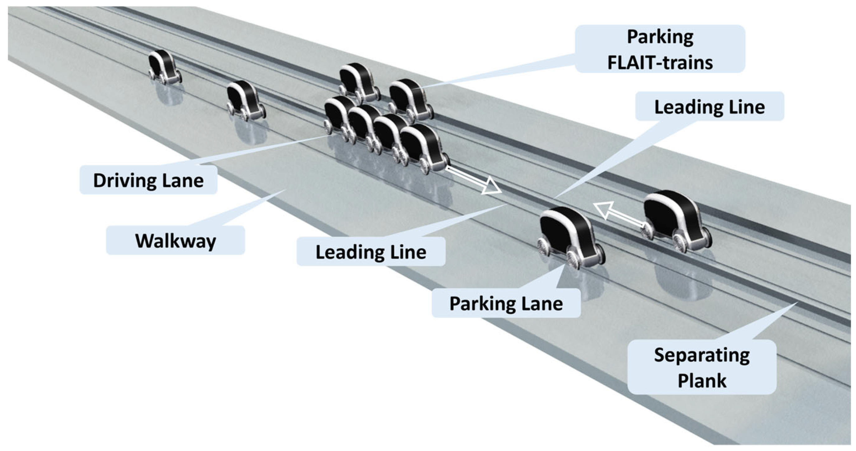
The FLAIT-train system, designed based on the vehicle specifications mentioned above, utilizes a unique approach for traffic flow. Each direction of travel on the classic tram track is divided into two sections: one for the parking lane and the other for the traffic of FLAIT. The FLAIT-trains operate fully autonomously, eliminating the dependence on the drivers’ working hours. Passengers can easily reserve a FLAIT-train at any time using their smartphones or other mobile devices.

One of the significant advantages of the FLAIT system is that passengers no longer need to walk to fixed stops. Instead, they can wait directly at the parking lane, reducing both the waiting time and walking distance to the stop. This innovative approach optimizes passenger convenience and enhances the overall transportation experience.

Figure 1 provides a graphical representation of the various advantages offered by the FLAIT-train system. Additionally,

Table 1. A comparison between five public transportation services [39].

	Tram	Typical On-Demand Transit	Taxi	FLAIT-Train	PRT
Route	Fixed	Flexible	Flexible	Fixed	Fixed
Stop	Fixed	w/o	w/o	w/o	Fixed
Schedule	Fixed	By request	By request	By request	By request
Ticket cost	Low	Medium	High	Low	Low
Mode	Shared	Shared	Non-shared	Shared 1	Shared 1
Seating capacity	>100	5–25	<7	2	2–4
Autonomous level	No	No	No	Automated	Fully
Track usage	Exclusive	Mixed	Mixed	Exclusive	Exclusive
Reservation	Not needed	Often needed	Not needed	Not needed 2	Not needed
Avg. speed [kph]	33.5 3	23 4	23 4	32	60 5

¹ Non-shared mode is provided with a surcharge. ² In principle, same as a taxi. ³ Average speed of trams in Duisburg according to [40]. ⁴ Average urban speed of automobile traffic in Düsseldorf according to [41]. ⁵ Planned average speed according to [42].

complements the characteristics of FLAIT-trains, making a comprehensive comparison with other transportation systems based on the table in [9].

2.4. Utilized Mathematical Approaches

2.4.1. Monte Carlo Method

The Monte Carlo method is a widely used computational technique with applications across various fields, ranging from physics and engineering to finance and computer science [43]. Named after the famous casino in Monaco, this method was first introduced by mathematicians John von Neumann and Stanislaw Ulam during the Manhattan Project in the 1940s [44].

The Monte Carlo method is a simulation-based approach that relies on random sampling to solve complex mathematical and statistical problems. The main idea behind the method is to generate many random samples from a given probability distribution and then use these samples to estimate the solution to the problem of interest. By repeating this process many times, Monte Carlo simulations provide a statistical approximation of the desired outcome with a certain confidence level.

One of the key advantages of the Monte Carlo method is its ability to handle problems with high dimensionality and uncertainty, where traditional analytical approaches may be computationally intractable or too restrictive. Additionally, it allows for the incorporation of various sources of randomness and complexity into the models, making it a versatile tool for analyzing real-world systems and processes [43].

In recent years, the Monte Carlo method has gained popularity in fields such as finance for pricing options, in physics for studying complex systems, and in engineering for risk analysis and reliability assessments. Its widespread adoption is due to its simplicity, flexibility, and the ability to provide accurate results even for intricate and non-linear problems [43].

This paper utilizes the Monte Carlo method to estimate passenger arrival times at bus stops in an on-demand public transport scenario. By generating random samples of passenger arrival times within a specified time window, valuable insights into the system’s behavior and performance can be obtained. Through Monte Carlo simulations, we aim to enhance the accuracy and reliability of our passenger models, contributing to a more efficient and optimized public transport system.

2.4.2. Convex Optimization Problem

As introduced in [45,46], convex optimization is a robust and widely used mathematical framework that deals with finding the best possible solution to a class of optimization problems. It plays a fundamental role in various fields such as engineering, finance, machine learning, and data science, where optimization tasks are prevalent.

The central focus of convex optimization is to optimize a convex objective function subject to a set of convex constraints. A function is considered convex if it satisfies a specific mathematical property that ensures its local and global minimums are the same. This property makes convex optimization particularly attractive, since it guarantees the existence of a unique and globally optimal solution.

In a convex optimization problem, the goal is to find the values of decision variables that minimize (or maximize) the convex objective function while satisfying the convex constraints. The decision variables represent the adjustable parameters of the problem, and their optimal values lead to the best possible outcome.

The process of solving convex optimization problems involves employing mathematical algorithms and techniques that efficiently navigate the solution space to identify the optimal solution. One of the most widely used methods is the interior-point method, which iteratively moves toward the interior of the feasible region while ensuring that each step leads to a feasible and improved solution.

Convex optimization has a wide range of applications, such as portfolio optimization in finance, parameter estimation in machine learning, trajectory planning in robotics, and resource allocation in engineering projects. Its ability to efficiently handle complex optimization tasks with guaranteed convergence to the global optimum makes it a vital tool in modern problem solving.

This paper employs convex optimization to estimate passengers’ alighting possibilities. By formulating the problem as a convex optimization task, the model efficiently determined the probabilities for passengers to alight at specific stops based on the given constraints.

3. Methodologies

3.1. Aim and Key Figures

The limited passenger seating capacity of each FLAIT vehicle raises the question of whether an appropriate number of FLAIT vehicles can effectively cover the system performance of conventional public transportation systems. As defined by [47], transportation system performance encompasses various quantitative operating characteristics, including the service frequency, speed, reliability, safety, capacity, and productivity. During rush hours, the passenger volume reaches its maximum, and it is essential for FLAIT vehicles to ensure that all passengers are transported to their destination with comparable or shorter waiting times.

To address this concern, simulations were conducted to determine the required number of FLAIT vehicles needed to match or exceed the performance of the conventional trams or buses based on the available statistical data. The goal is to assess whether the resulting number of FLAIT vehicles is feasible for both operational and economic reasons. In the real FLAIT-train system, the passengers can board and alight at any point along the FLAIT tracks without fixed stops, providing additional flexibility and convenience.

However, in this paper, the main objective is to investigate whether the FLAIT-trains can effectively handle the passenger volume currently served by trams or buses based on the available statistical data. To achieve this goal, the simulations with FLAIT-trains still involve picking up passengers from the tram or bus stops without considering the full advantage of the flexible stops that FLAIT-trains offer.

One advantage of FLAIT-trains compared to conventional public transportation systems is the elimination of transfer. However, due to the limitation of unavailable statistical data for the simulative analysis, passenger transfers cannot be considered within the scope of this paper. The limitation presents another constraint of the study.

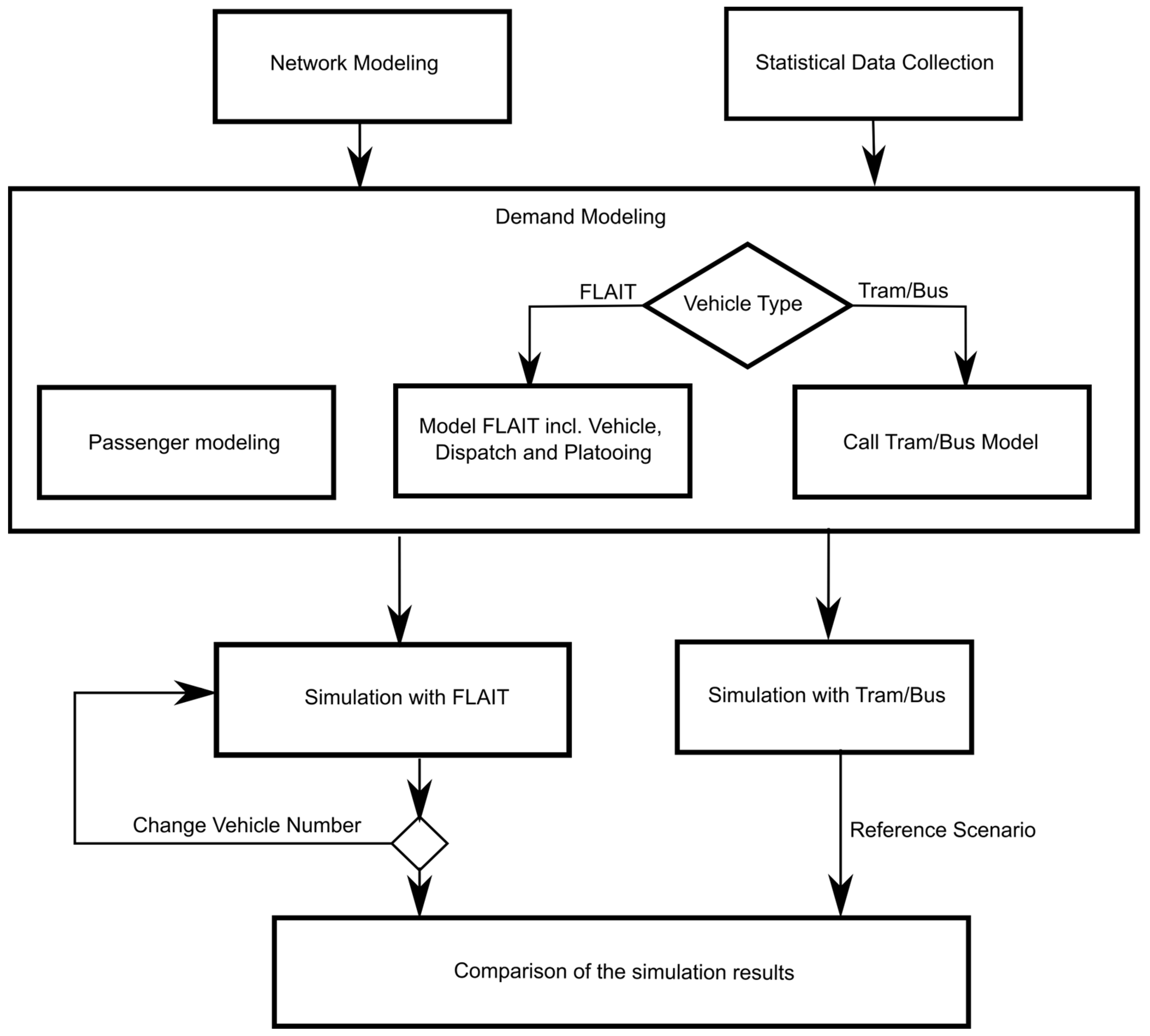
For the analysis, all statistical data provided by DVG were first summarized and analyzed. Furthermore, the scenario, including streets and bus stops, was modeled in SUMO. In the next step, passengers were modeled in SUMO based on the statistical data, as well as related vehicles such as buses and FLAIT-trains. The modeling of the related components in SUMO will be explained in more detail in Section 4. After the modeling, a reference simulation using the bus model was conducted to obtain the performance data of the current state. Subsequently, iteration simulations for the FLAIT-trains were carried out by varying the number of FLAIT-trains. The results analysis and comparison between the two transportation modes were executed in MATLAB (version 24.1) and will be depicted in Section 5. The methodology used for this analysis is graphically described in Figure 2, as introduced in [39].

However, it is important to note that in these simulations, the passengers are still assumed to be picked up from the traditional tram or bus stops, and the full potential of the FLAIT system’s flexible stops is not yet taken into account.

The evaluation of the system performance in this paper is based on the four key performance figures, which are as follows:

• Average waiting time per passenger;
• Maximum waiting time for a single passenger;
• Average in-vehicle time per passenger;
• Average occupancy rate of the vehicles.

3.1.1. Average Waiting Time per Passenger

Indeed, the average waiting time per passenger ($t_{W,mean}$) is a crucial metric that directly reflects the reliability and quality of the public transport service, as noted in [48]. This paper also considers $t_{W,mean}$ as a significant evaluation criterion.

To calculate $t_{W,mean}$, the waiting time of each individual passenger ($t_{W,i}$) is recorded. The total number of passengers transported is denoted by $n_p$. The average waiting time per passenger is then obtained by dividing the sum of all individual waiting times by the total number of passengers:

$$t_{W,mean}=\frac{\sum _{i=1}^{n_p}{t}_{W,i}}{n_p}.$$

(1)

This formula allows for the determination of the average waiting time experienced by passengers throughout the entire simulation or study period. By using this metric, the paper aims to assess the overall service reliability and passenger satisfaction in both the conventional public transportation and FLAIT-train systems.

3.1.2. Maximum Waiting Time of a Single Passenger

In on-demand public transport, the maximum waiting time of a single passenger ($t_{W,max}$) is another crucial indicator of the service quality, alongside the average waiting time [49,50]. This paper recognizes the importance of $t_{W,max}$ and includes it as an evaluation criterion.

To compute $t_{W,max}$, the waiting time of each individual passenger is recorded as $t_{W,i}$. The total number of passengers transported is represented by $n_p$. The maximum waiting time of a passenger is then determined by selecting the longest waiting time among all passengers:

$$t_{W,max}=\max (t_{W,1}, t_{W,2}, \cdots ,t_{W,n_p}).$$

(2)

This metric allows for the identification of the most extended waiting time experienced by any passenger during the simulation or study period. It highlights the potential instances of prolonged waiting, which can be critical for passenger satisfaction and the overall service performance. By incorporating $t_{W,max}$, the paper aims to assess the reliability and consistency of both the conventional public transportation and FLAIT-train systems in serving individual passengers.

3.1.3. Average In-Vehicle Time per Passenger

Indeed, the average in-vehicle time per passenger ($t_{J,mean}$) is a critical metric in assessing the public transport service reliability, and it has been recognized as such in previous studies, including in [48]. This paper also considers $t_{J,mean}$ as an essential evaluation factor.

To calculate $t_{J,mean}$, the in-vehicle time for each individual passenger is recorded as $t_{J,i}$. The total number of passengers transported is represented by $n_p$. The average in-vehicle time per passenger is then derived using following formula:

$$t_{J,mean}=\frac{\sum _{i=1}^{n_p}{t}_{J,i}}{n_p}.$$

(3)

This metric measures the average time spent by passengers on their journey, exclusively while onboard the tram/bus or FLAIT-train. It provides valuable insights into the transport system’s efficiency and the passengers’ overall travel experience. By incorporating $t_{J,mean}$, the paper aims to analyze the in-vehicle experiences of passengers using both modes of transport and assess their comparative reliability and efficiency.

3.1.4. Average Occupancy Rate of Vehicles

Additionally, to complement the aforementioned key performance figures, this paper introduced the average occupancy rate of the vehicles as a means to compare the usage efficiency between bus and FLAIT-train transit systems. As the number of the FLAIT-trains increased, there was a corresponding decrease in the average and maximum waiting times, as well as the average in-vehicle time. However, it is expected that the occupancy rate of the vehicles would decrease due to the increased passenger capacities available.

In this paper, the average occupancy rate of the vehicles was considered as long as at least one passenger was transported by a vehicle. This key performance figure was determined using the following formula:

$${OCC}_{mean}=\frac{\sum _{t=t_0}^{t_e}\frac{n_{P,t_i}}{C_{P,V} · n_V}}{\sum _{t=t_0}^{t_e}{t}_i}.$$

(4)

To calculate the average occupancy rate of the vehicles, the occupancy rate of each time point was summed and divided by the total duration for which at least one passenger was transported by a vehicle. The occupancy rate of the time point ($t_i$) was computed by dividing the number of transported passengers ($n_{P,t_i}$) by the passenger capacity of each vehicle ($C_{P,V}$) and the total number of vehicles in the fleet ($n_V$).

4. Scenario Concept Design

4.1. Simulation Tool

For simulating the scenario involving conventional public transportation systems and FLAIT-trains, the researchers utilized SUMO (Simulation of Urban Mobility, version 11.2.0), an open-sourced microscopic traffic simulation software. The decision to use SUMO was based on the specific requirements of the simulations and the extensive analyses comparing various simulation software options [51,52].

By leveraging SUMO, the researchers were able to accurately model and analyze the transportation scenarios involving conventional public transportation systems and FLAIT-trains, taking into account factors such as the passenger volumes, waiting times, in-vehicle times, and other performance indicators. SUMO’s capabilities and flexibility allowed for the comprehensive evaluation of the FLAIT system and its comparison with conventional public transportation systems, enabling valuable insights and conclusions to be drawn from simulation results.

4.2. Simulation Scenario

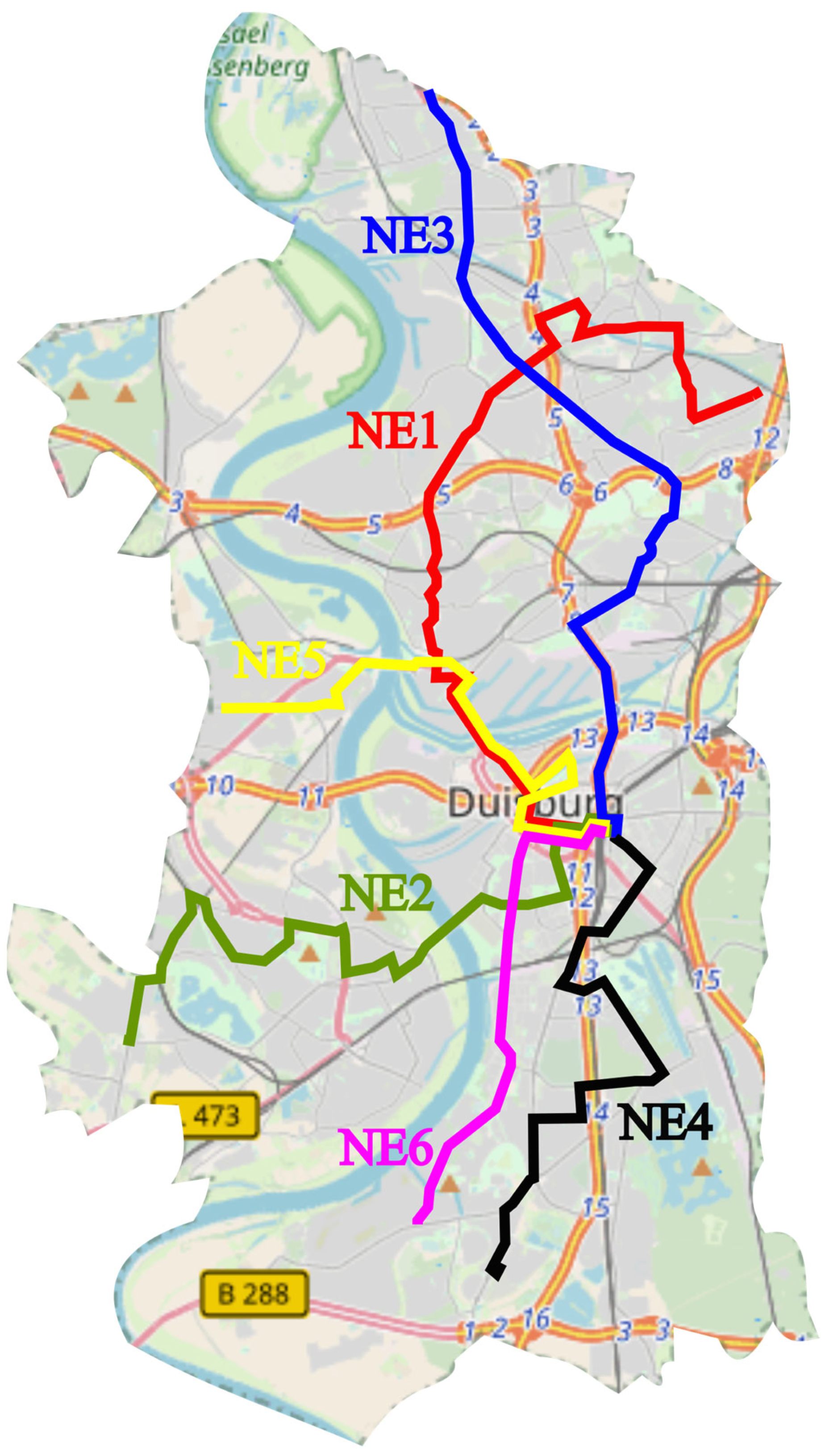
Currently, there are six night bus routes available in Duisburg, as shown in

Table 2. Duisburg night bus routes.

Bus Route	From	To	Stops	Duration in [min]
NE1	Buschhauser Str.	DU-Hbf East Entrance	44	64
	DU-Hbf East Entrance	Buschhauser Str.	44	63
NE2	Rumeln Town Hall	DU-Hbf East Entrance	29	53
	DU-Hbf East Entrance	Rumeln Town Hall	29	54
NE3	Watereck	DU-Hbf East Entrance	23	41
	DU-Hbf East Entrance	Watereck	23	38
NE4	St. Anna Hospital	DU-Hbf East Entrance	28	34
	DU-Hbf East Entrance	St. Anna Hospital	27	39
NE5	Hochheide Market	DU-Hbf East Entrance	25	38
	DU-Hbf East Entrance	Hochheide Market	25	42
NE6	Mannesmann Gate 2	DU-Hbf East Entrance	20	33
	DU-Hbf East Entrance	Mannesmann Gate 2	20	34

. The night bus service, operated by DVG, runs daily from 11 p.m. to 5 a.m., and on weekends, it operates until 8 a.m. The bus stops for these six routes are distributed throughout the entire city. Each bus route has its final stop at Duisburg’s central railway station, providing passengers with the opportunity to transfer to other bus routes at the station.

During nighttime, the number of passengers is typically lower compared to daytime. As a result, the time interval between two night buses is usually longer than during the day. Based on the current timetable, the buses depart once every hour. Consequently, passengers are unable to return home at any time they wish. Instead, they must make their way to the bus stop shortly before the bus is scheduled to arrive.

However, this particular use case is well suited for on-demand vehicles. On-demand vehicles typically have lower passenger capacities than conventional buses, allowing for a more flexible service when serving fewer passengers. This flexibility enables the on-demand vehicles to provide a tailored and responsive service based on the specific needs of the passengers.

In the simulative analysis, all six night bus routes in Duisburg have been included. The details of these routes, including their end station, number of stops, and duration in both directions, have been compiled in Table 2. It is important to note that for the bus route “NE3”, there are stops located in the city of Dinslaken and outside Duisburg, which are not considered within the scope of this paper. The visualization of all the bus routes can be found in Figure 3.

Similar to the other scenarios, the simulations were carried out with varying numbers of FLAIT vehicles. Furthermore, the passenger capacity of each FLAIT vehicle was considered to assess its influence on transportation performance. A reference simulation was conducted in the same scenario using buses and following the actual timetable to facilitate a comparison with the conventional transportation system.

4.3. Vehicle Models

4.3.1. Bus

In this paper, the existing vehicle class “Bus” in SUMO was employed to model and simulate buses. The default parameters of the SUMO model source code were used directly. The bus model was incorporated in the scenario “Night Bus Routes in Duisburg”, which encompasses the entire Duisburg area. Therefore, no additional speed limitation was set for the buses in this scenario.

4.3.2. FLAIT

The FLAIT vehicles were represented as a new vehicle class named “Flait” in SUMO. The modeling process involved a combination of existing models for trams and taxis in SUMO. To emulate trams, the FLAIT vehicles were restricted to driving exclusively on the tram tracks, denoted by the SUMO road type “railway.tram”. The FLAIT vehicles would come to a halt at the last exit point of a passenger and only resume movement upon receiving the next passenger reservation. Since the FLAIT system’ss application focused on an urban scenario, the FLAIT model’s driving speed was restricted to 50 kph (kilometer per hour), which represents the maximum speed allowed within German cities.

4.4. Passengers

In the simulations, different passenger groups were modeled using the SUMO function “personFlow” [53]. The following parameters characterized each passenger group:

• The time (to the second) when the first passenger of this group departs;
• The time (to the second) when the last passenger of the group departs;
• The number of members in the group;
• The street ID where the group departs from;
• The stop where the group waits for tram/bus or FLAIT-train;
• The destination street ID where the group alights.

As the focus of this paper is on transport performance, the passenger walking distance and time were not considered as criteria. Therefore, it was assumed that passengers would send out FLAIT reservations while waiting at the bus stops, without considering the walking distances and times for the passengers.

In the scenario “Night Bus Routes in Duisburg”, the passenger volume modeling relies on the statistical data obtained from Duisburger Verkehrsgesellschaft AG (DVG) for the current bus routes NE1 to NE6. These datasets were used as a reference to simulate the passenger demand and distribution for the proposed FLAIT-train system in comparison to the existing bus routes.

To accurately represent the demand for transportation, the highest passenger volume within an hour was determined for each bus route from the DVG database. These peak passenger volumes were then summarized to create the datasets for the simulation. The purpose of using the highest passenger volumes is to simulate the scenario with the most demanding transport capacity requirement, representing a worst-case scenario for the FLAIT-train system.

The statistical data obtained from the DVG provide information about the number of boarding and alighting passengers at each stop along the six bus routes. However, the following pieces of information are missing:

• From what time did the passenger wait for the bus?

The data do not include the exact waiting times for individual passengers at each bus stop. The waiting time of each passenger is essential to determine factors such as the average waiting time and maximum waiting time per passenger, which are crucial performance indicators for public transportation systems.

• At which bus stop will the boarding passenger alight?

The dataset does not specify each boarding passenger’s destination or alighting bus stop. This information is vital to simulate the passenger journey from the boarding point to the destination and accurately assess the transportation system’s performance, for example, the total in-vehicle time.

• At which bus stop has the alighting passenger been boarded?

Similarly, the dataset does not indicate where the alighting passenger initially boarded the bus. This information is necessary to determine the complete passenger journey, including the boarding and alighting bus stops, to analyze the travel patterns and evaluate the transportation system’s performance.

4.4.1. Estimation of Passenger Arrival Times at Bus Stops

In the nighttime, the passengers are often on the move and may want to return home at any given time. However, due to the long headway of night buses, they are required to wait, for instance, at a bar until shortly before the bus arrives based on the timetable.

Therefore, accurately estimating the passenger arrival time at bus stops using models in the literature, such as in [48], is challenging. In this paper, the Monte Carlo method, as described in Section 2.4.1, was applied to address this issue. The arrival time at a bus stop of each passenger has been generated as a random number between 11 pm and 12 am.

4.4.2. Estimations of Passengers’ Boarding and Alighting Bus Stops

The passengers’ boarding and alighting bus stops were estimated as the solution of an optimization problem, as described in [54]. The relationship between the numbers of boarding and alighting passengers at a bus stop was formulated using the following equation:

$$a_i={\sum }_{i=1}^n{(x}_{j-i}·e_j),$$

(5)

where:

• $a_i$ represents the number of alighting passengers at bus stop $i$;
• $e_j$ denotes the number of boarding passengers at bus stop $j$;
• $x_{j-i}$ represents the alighting possibility at bus stop $i$.

If all bus stops are considered, the equation system above can be summarized and represented in a matrix format:

$$\left(\begin{array}{c}{a}_1\\ a_2\\ \begin{array}{c}{a}_3\\ ⋮\\ a_n\end{array}\end{array}\right)=\left(\begin{array}{ccc}\begin{array}{ccc}\begin{array}{c}{x}_{1-1}\\ x_{1-2}\\ x_{1-3}\end{array}& \begin{array}{c}{x}_{2-1}\\ x_{2-2}\\ x_{2-3}\end{array}& \begin{array}{c}{x}_{3-1}\\ x_{3-2}\\ x_{3-3}\end{array}\end{array}& \cdots & \begin{array}{c}{x}_{m-1}\\ x_{m-2}\\ x_{m-3}\end{array}\\ ⋮& \ddots & ⋮\\ \begin{array}{ccc}{x}_{1-n}& x_{2-n}& x_{3-n}\end{array}& \cdots & x_{m-n}\end{array}\right)\times \left(\begin{array}{c}{e}_1\\ e_2\\ \begin{array}{c}{e}_3\\ ⋮\\ e_m\end{array}\end{array}\right),$$

(6)

where:

• $a_1, a_2, \dots , a_n$ represent the alighting passengers at bus stop $1, 2, \dots , n$, respectively;
• $x_{1-1}, x_{1-2}, \dots , x_{m-n}$ represent the alighting possibility at each bus stop;
• $e_1, e_2, \dots , e_m$ represent the boarding passengers at bus stop $1, 2, \dots , m$, respectively.

It is derived from (6) to a standard form for an optimization problem as follows:

$$\left(\begin{array}{ccc}\begin{array}{ccc}\begin{array}{c}{x}_{1-1}\\ x_{1-2}\\ x_{1-3}\end{array}& \begin{array}{c}{x}_{2-1}\\ x_{2-2}\\ x_{2-3}\end{array}& \begin{array}{c}{x}_{3-1}\\ x_{3-2}\\ x_{3-3}\end{array}\end{array}& \cdots & \begin{array}{c}{x}_{m-1}\\ x_{m-2}\\ x_{m-3}\end{array}\\ ⋮& \ddots & ⋮\\ \begin{array}{ccc}{x}_{1-n}& x_{2-n}& x_{3-n}\end{array}& \cdots & x_{m-n}\end{array}\right)\times \left(\begin{array}{c}{e}_1\\ e_2\\ \begin{array}{c}{e}_3\\ ⋮\\ e_m\end{array}\end{array}\right)-\left(\begin{array}{c}{a}_1\\ a_2\\ \begin{array}{c}{a}_3\\ ⋮\\ a_n\end{array}\end{array}\right)=\left(\begin{array}{c}0\\ 0\\ \begin{array}{c}0\\ ⋮\\ 0\end{array}\end{array}\right).$$

(7)

To determine the possibilities $x_{1-1}, x_{1-2}, \dots , x_{m-n}$, the optimization problem is formulated as follows:

$$\begin{array}{c}\underset{x\in {\mathbb{R}}^n}{\min }({\left(x_{1-1}\times e_1+x_{2-1}\times e_2+\cdots +x_{m-1}\times e_m-a_1\right)}^2+\dots \\ \hspace{1em}\hspace{1em}\hspace{1em}\hspace{1em}\hspace{1em}\hspace{1em}\hspace{1em}\hspace{1em}\hspace{1em}+{\left(x_{1-n}\times e_1+x_{2-n}\times e_2+\cdots +x_{m-n}\times e_m-a_n\right)}^2),\end{array}$$

(8)

subject to the constraint:

$${\sum }_{k=1}^m{x}_{k-i}-1=0 \mathrm{for} i=1, 2, 3, \dots , n$$

(9)

Using the available Python (version 3.10.12) toolbox “CVXPY”, it is possible to solve this convex optimization problem as introduced in Section 2.4.2. Additionally, with other available Python toolboxes, the passenger models can be directly exported in the specified XML format, which can be directly utilized in SUMO simulations [54]. This allows for the efficient and seamless integration of the passenger models into the simulation environment.

4.5. Flexible Platooning

In the context of this paper, a toolbox called “Simpla” was utilized in SUMO to simulate flexible vehicle platooning. The development of this toolbox was based on the work of [55]. The car-following model employed in the simulations was the Krauss model, as introduced in [56]. As the FLAIT vehicles are highly autonomous vehicles, the model of perfect drivers was utilized in the simulations. This choice allowed for the accurate representation of the FLAIT vehicles’ behaviors in the platooning system, taking advantage of their advanced automation capabilities.

5. Simulation Results Based on Statistical Data

In the scenario presented in Section 4, night transportation using different modes of transport was simulated. In addition to the simulation involving traditional buses, simulations were conducted with different numbers of FLAIT vehicles, ranging from 10 to 100 FLAIT vehicles. The delta value between the considered numbers of FLAIT vehicles was set to 10, providing a comprehensive analysis of the performance with an increasing FLAIT vehicle counts.

Furthermore, alongside the simulations involving different numbers of FLAIT vehicles, the impact of passenger capacities on the transportation performance was also analyzed. The simulations were conducted considering passenger capacities of 5, 10, 15, and 20 passengers per FLAIT-train. This analysis allowed for a comprehensive assessment of how varying passenger capacities affect the overall transportation performance.

In the analysis, the results for night buses are represented in magenta. Additionally, the results for FLAIT-trains are depicted in different colors: cyan for a passenger capacity of 2, red for a passenger capacity of 5, green for a passenger capacity of 10, blue for a passenger capacity of 15, and black for a passenger capacity of 20. This comprehensive approach enables a detailed understanding of the performances of both buses and FLAIT-trains with the increased seating places.

5.1. Average Waiting Time per Passenger

5.1.1. Exploring the Passenger Capacity of Two Seats

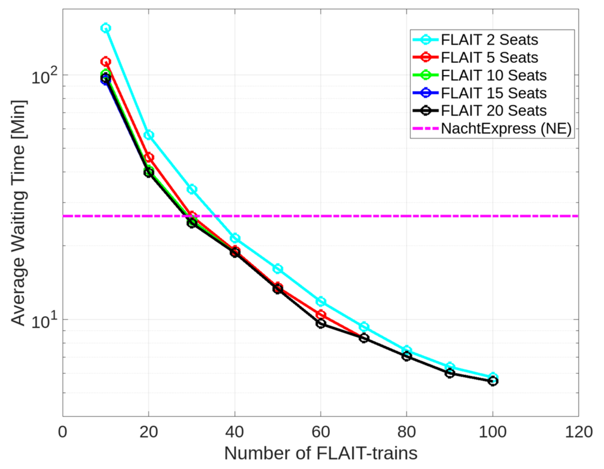
In the reference simulations with conventional buses, the average waiting time was calculated using Formula (1) and yielded similar values, specifically 26.5 min per passenger.

In the case of FLAIT-trains, the average waiting time displayed a relationship with the number of FLAIT-trains, as illustrated in Figure 4, using a logarithmic scale. The average waiting time exhibited a consistent decrease as the number of FLAIT-trains increased.

From 10 to 30 FLAIT-trains, the average waiting times were higher compared to the reference simulation with buses. Specifically, the average waiting times for these FLAIT ranges were approximately 155.3 min, 56.6 min, and 34.0 min. When compared to the reference simulation, the average waiting time for FLAIT-trains was longer than that of conventional buses by 486.0% (10 FLAIT-trains), 113.6% (20 FLAIT-trains), and 28.3% (30 FLAIT-trains), respectively.

With 40 to 100 FLAIT vehicles, the average waiting time decreased compared to the reference simulation, with values of 21.5 min, 16.1 min, 11.8 min, 9.3 min, 7.4 min, 6.4 min, and 5.8 min. The improvements achieved by FLAIT vehicles in comparison to the reference simulation were 18.9% (40 FLAIT-trains), 39.2% (50 FLAIT-trains), 55.5% (60 FLAIT-trains), 64.9% (70 FLAIT-trains), 72.1% (80 FLAIT-trains), 75.8% (90 FLAIT-trains), and 78.1% (100 FLAIT-trains), respectively. These percentage improvements were calculated using the formula $\frac{t_{w,mean,Bus}-t_{w,mean, FLAIT}}{t_{w,mean,Bus}}\times 100$.

5.1.2. Exploring the Increased Passenger Capacities

To assess the impact of increased passenger capacities on the average waiting time, additional simulations were performed with passenger capacities of 5, 10, 15, and 20, respectively. The outcomes of these simulations are incorporated into Figure 4.

According to the simulation results, there was a noticeable decrease in the average waiting time per passenger as the passenger capacity of each vehicle increased. Specifically, when each vehicle had a seating capacity of five, there was a noteworthy decrease in the average waiting time compared to a passenger capacity of two. With the presence of 10 FLAIT-trains, the average waiting time reduced from 155.3 min to 113.3 min, representing a 27.0% decrease. Similarly, with 20 FLAIT-trains, the average waiting time improved from 56.6 min to 46.0 min, reflecting an 18.7% improvement. Furthermore, with 30 to 100 FLAIT-trains, the average waiting time for five seating places in each FLAIT-train ranged from 26.8 min (30 FLAIT-trains) to 5.6 min (100 FLAIT-trains). The improvements achieved in each case were 21.2% (30 FLAIT-trains), 11.6% (40 FLAIT-trains), 16.1% (50 FLAIT-trains), 11.9% (60 FLAIT-trains), 9.7% (70 FLAIT-trains), 5.4% (80 FLAIT-trains), 6.3% (90 FLAIT-trains), and 3.4% (100 FLAIT-trains), respectively.

As the passenger capacities increased further from 5 to 20, the improvements in the average waiting time per passenger decreased. Particularly, from 70 to 100 FLAIT-trains, no improvements were achieved, with average waiting times remaining at 8.4 min (70 FLAIT-trains), 7.0 min (80 FLAIT-trains), 6.0 min (90 FLAIT-trains), and 5.6 min (100 FLAIT-trains).

From 40 to 60 FLAIT-trains, there was a noticeable improvement in the average waiting time after increasing the passenger capacity from 5 to 10. The average waiting time decreased from 19.0 to 18.7 min (40 FLAIT-trains), from 13.5 to 13.3 min (50 FLAIT-trains), and from 10.4 to 9.6 min (60 FLAIT-trains). However, no further improvements were observed when increasing the passenger capacities from 10 to 20.

With 20 or 30 FLAIT-trains, there was an improvement in the average waiting time after increasing the passenger capacities from 5 to 15. Specifically, the average waiting time for 20 FLAIT-trains decreased from 46.0 min to 40.7 min, and further to 39.8 min. Similarly, for 30 FLAIT-trains, the average waiting time decreased from 26.8 min to 25.4 min, and further to 24.7 min. However, no further improvements were observed when increasing the passenger capacities from 15 to 20.

With 10 FLAIT-trains, the average waiting times reduced from 113.3 min to 100.7 min, further to 97.0 min, and ultimately to 94.9 min after increasing the passenger capacities from 5 to 20. The impact of the number of FLAIT vehicles and passenger capacities is summarized in

Table 3. Impact of passenger capacities on average waiting time in [min].

	2 SPs	5 SPs	10 SPs	15 SPs	20 SPs	NE
10 FLAIT-trains	155.3	113.3	100.7	97.0	94.9	26.5
20 FLAIT-trains	56.6	46.0	40.7	39.8	39.8
30 FLAIT-trains	34.0	26.8	25.4	24.7	24.7
40 FLAIT-trains	21.5	19.0	18.7	18.7	18.7
50 FLAIT-trains	16.1	13.5	13.3	13.3	13.3
60 FLAIT-trains	11.8	10.4	9.6	9.6	9.6
70 FLAIT-trains	9.3	8.4	8.4	8.4	8.4
80 FLAIT-trains	7.4	7.0	7.0	7.0	7.0
90 FLAIT-trains	6.4	6.0	6.0	6.0	6.0
100 FLAIT-trains	5.8	5.6	5.6	5.6	5.6

.

5.2. Maximum Waiting Time of a Single Passenger

5.2.1. Exploring the Passenger Capacity of Two Seats

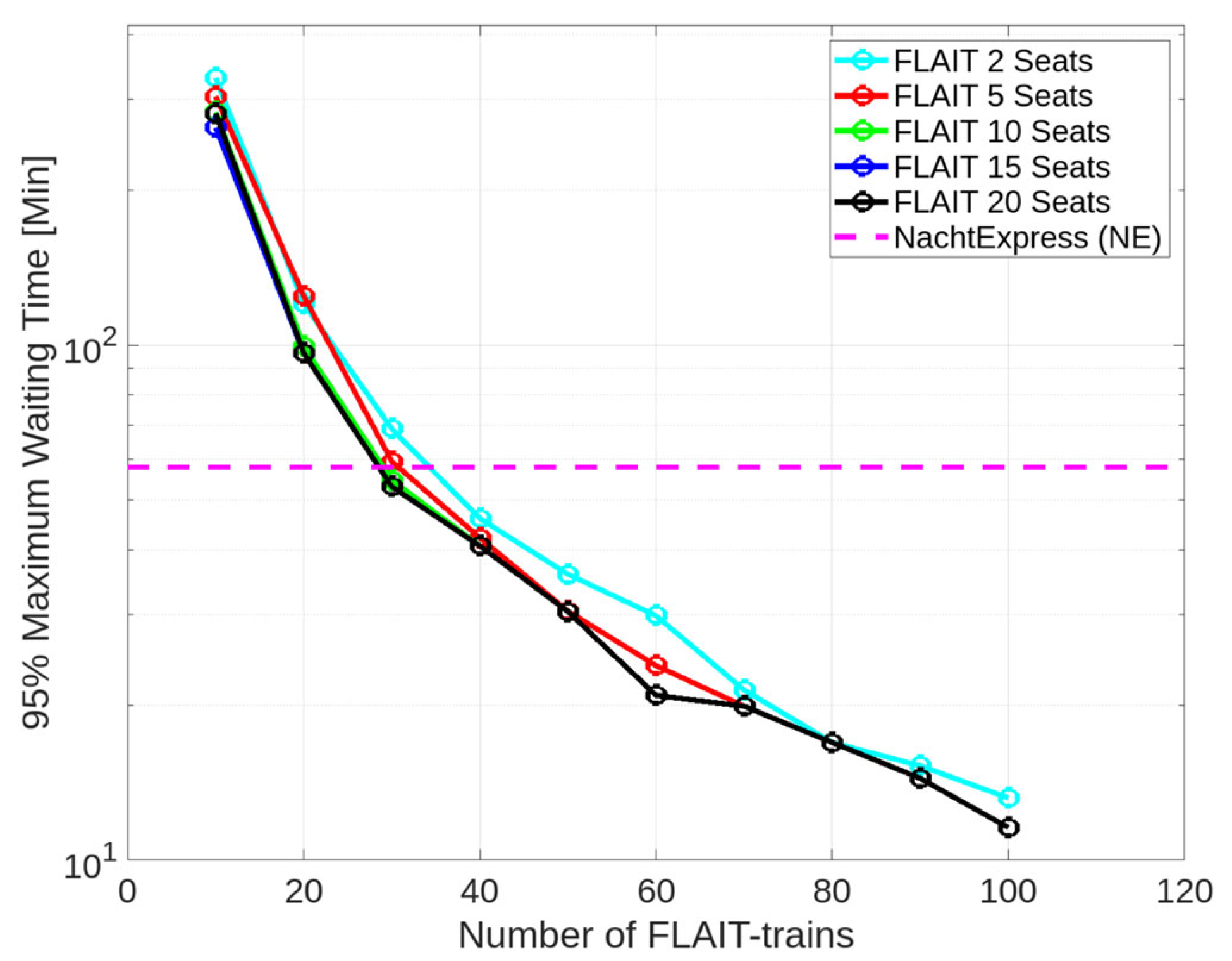
In [40], the analysis focused on the absolute maximum waiting time of a single passenger, acknowledging the potential influence of the utilized dispatching algorithm. To ensure a robust evaluation and comparison between buses and FLAIT-trains, the 95% maximum waiting time was considered as a more representative metric. This approach allowed for the comprehensive assessment of both transportation modes while accounting for any variations introduced by the dispatching algorithm.

In the reference simulation with night buses, the 95% maximum waiting time for a single passenger was calculated using the provided Formula (2). Based on the simulation results, the 95% maximum waiting time of a bus was determined to be 57.9 min.

Similar to the average waiting time, the 95% maximum waiting time for FLAIT-trains showed similar dependencies on the number of FLAIT-trains. These dependencies are visualized as logarithmic coordinates in Figure 5.

Between 10 and 30 FLAIT-trains, the 95% maximum waiting times were higher compared to the reference simulation with buses. Specifically, the 95% maximum waiting times for these FLAIT ranges were approximately 329.8 min, 120.3 min, and 68.8 min. When compared to the reference simulation, the average waiting time for FLAIT-trains was longer than that of conventional buses by 469.6% (10 FLAIT-trains), 107.8% (20 FLAIT-trains), and 18.8% (30 FLAIT-trains), respectively.

With 40 to 100 FLAIT-trains, there was a decrease in the 95% maximum waiting time compared to the reference simulation, with values of 46.0 min, 35.9 min, 29.8 min, 21.4 min, 16.9 min, 15.3 min, and 13.2 min. The improvements achieved by FLAIT-trains in comparison to the reference simulation were 20.6% (40 FLAIT-trains), 38.0% (50 FLAIT-trains), 48.5% (60 FLAIT-trains), 63.0% (70 FLAIT-trains), 70.8% (80 FLAIT-trains), 73.6% (90 FLAIT-trains), and 77.2% (100 FLAIT-trains), respectively.

5.2.2. Exploring the Increased Passenger Capacities

Similar to the average waiting time, the additional simulation results for the 95% maximum waiting time are incorporated into Figure 5 for the increased seating capacities from 5 to 20.

Based on the simulation results, there was a noticeable decrease in the 95% maximum waiting time per passenger as the passenger capacity of each vehicle increased. Specifically, when each vehicle had a seating capacity of five, there was a significant reduction in the 95% maximum waiting time compared to a passenger capacity of two. With 10 FLAIT-trains, the 95% maximum waiting time decreased from 329.8 min to 304.0 min, representing a 7.8% decrease. With 30 to 70 FLAIT-trains and 90 to 100 FLAIT-trains, the 95% maximum waiting time for five seating places in each FLAIT-train ranged from 64.2 min (30 FLAIT-trains) to 13.2 min (100 FLAIT-trains). The improvements achieved in each case, compared to a passenger capacity of two, were 13.7% (30 FLAIT-trains), 8.0% (40 FLAIT-trains), 15.3% (50 FLAIT-trains), 19.8% (60 FLAIT-trains), 7.0% (70 FLAIT-trains), 5.9% (90 FLAIT-trains), and 12.1% (100 FLAIT-trains), respectively. However, with 20 and 80 FLAIT-trains, the 95% maximum waiting time showed no improvement.

As the passenger capacities increased further from 5 to 20, the 95% maximum waiting times with 10 FLAIT-trains decreased from 304.0 min to 282.9 min, further to 281.6 min, and ultimately to 264.3 min.

With 20 or 30 FLAIT-trains, there was an improvement in the 95% maximum waiting time by increasing the passenger capacities from 5 to 15. Specifically, the 95% maximum waiting time decreased from 124.5 min to 99.5 min, and further to 96.4 min with 20 FLAIT-trains. With 30 FLAIT-trains, the 95% maximum waiting time decreased from 59.4 min (5 seating places) to 54.7 min (10 seating places), and further to 53.1 min (15 seating places). However, no further improvements were observed in each case when increasing the passenger capacities from 15 to 20.

With 40 or 60 FLAIT vehicles, the 95% maximum waiting time was improved by increasing the passenger capacity from 5 to 10. Specifically, the 95% maximum waiting time for 40 FLAIT vehicles decreased from 42.3 to 40.8 min. With 60 FLAIT vehicles, the 95% maximum waiting time reduced from 23.9 min to 20.9 min. However, no further improvements were observed when increasing the passenger capacities from 10 to 20.

Particularly with 50 FLAIT-trains and from 70 to 100 FLAIT-trains, no improvements were achieved by increasing the passenger capacities from 5 to 20, as the 95% maximum waiting times remaining at 30.4 min (50 FLAIT-trains), 19.9 min (70 FLAIT-trains), 16.9 min (80 FLAIT-trains), 14.4 min (90 FLAIT-trains), and 11.6 min (100 FLAIT-trains). The impact of the number of FLAIT vehicles and passenger capacities is summarized in

Table 4. Impact of passenger capacities on 95% maximum waiting time in [min].

	2 SPs	5 SPs	10 SPs	15 SPs	20 SPs	NE
10 FLAIT-trains	329.8	304.0	282.9	281.6	264.3	57.9
20 FLAIT-trains	120.3	124.5	99.5	96.4	96.4
30 FLAIT-trains	68.8	59.4	54.7	53.1	53.1
40 FLAIT-trains	46.0	42.3	40.8	40.8	40.8
50 FLAIT-trains	35.9	30.4	30.4	30.4	30.4
60 FLAIT-trains	29.8	23.9	20.9	20.9	20.9
70 FLAIT-trains	21.4	19.9	19.9	19.9	19.9
80 FLAIT-trains	16.9	16.9	16.9	16.9	16.9
90 FLAIT-trains	15.3	14.4	14.4	14.4	14.4
100 FLAIT-trains	13.2	11.6	11.6	11.6	11.6

.

5.3. Average In-Vehicle Time per Passenger

5.3.1. Exploring the Passenger Capacity of Two Seats

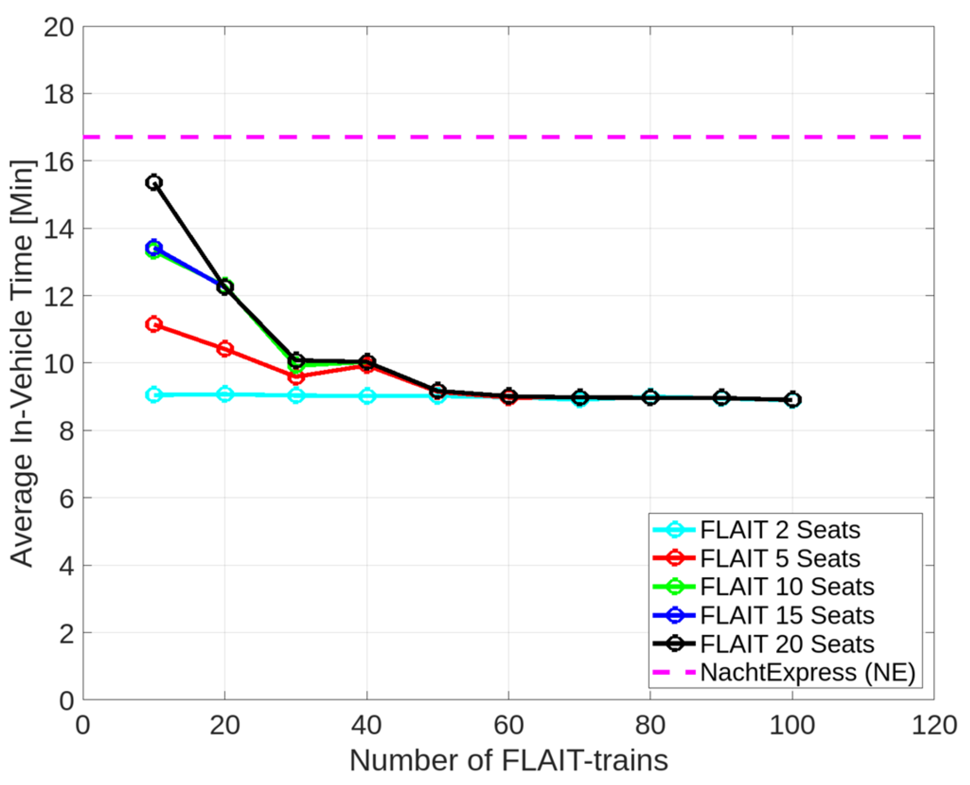
The average in-vehicle time for FLAIT-trains was found to be shorter than bus trips due to the absence of intermediate stops, as depicted in Figure 6. Using Formula (3), the average in-vehicle time per bus passenger was calculated. Depending on the departure and arrival stops, this resulted in approximately 16.7 min.

In comparison to the reference value from the bus simulations, the trips using 10 to 100 FLAIT-trains took between 8.9 min and 9.1 min. By eliminating the intermediate stops, passengers were able to reduce their travel time by approximately 45.5%.

5.3.2. Exploring the Increased Passenger Capacities

To investigate the impact of increased passenger capacities on the average in-vehicle time, additional iteration simulations were conducted with passenger capacities of 5, 10, 15, and 20 seating places, respectively. The simulation results are shown in Figure 6.

As the passenger capacities increased, the number of intermediate stops also increased, leading to longer average in-vehicle times per passenger. With 10 FLAIT-trains, the average in-vehicle time increased from 9.1 min to 11.1 min, further to 13.3 min, 13.4 min, and ultimately to 15.4 min. However, even with a seating capacity of 20, the average in-vehicle time of FLAIT-trains is still lower than that of conventional buses by 7.8%.

For 20 FLAIT-trains, there was an increase in the average in-vehicle time as the passenger capacities increased from 2 to 15. Specifically, the average in-vehicle time increased from 9.1 min (2 seating places) to 10.4 min (5 seating places), further to 12.3 min (10 seating places), and ultimately to 12.2 min (15 seating places). However, no further change was observed when increasing the passenger capacities from 15 to 20.

Particularly with from 70 to 100 FLAIT-trains, no improvements were achieved, with average waiting times remaining at 8.4 min (70 FLAIT-trains), 7.0 min (80 FLAIT-trains), 6.0 min (90 FLAIT-trains), and 5.6 min (100 FLAIT-trains).

For 30 or 40 FLAIT-trains, a significant increase in the average in-vehicle time was observed by increasing the passenger capacity from 2 to 5. Specifically, the average in-vehicle time increased from 9.0 min to 9.8 min and 9.9 min, respectively. However, the further changes were within a range of 3.2% (30 FLAIT-trains) and 1.0% (40 FLAIT-trains) as the passenger capacity increased from 5 to 20.

With 50 to 100 FLAIT-trains, no significant changes in the average in-vehicle time were observed, and the value changes were within a range of 2.3%. The impact of the number of FLAIT-trains and passenger capacities on the average in-vehicle time is summarized in

Table 5. Impact of passenger capacities on average in-vehicle time in [min].

	2 SPs	5 SPs	10 SPs	15 SPs	20 SPs	NE
10 FLAIT-trains	9.1	11.1	13.3	13.4	15.4	16.7
20 FLAIT-trains	9.1	10.4	12.3	12.2	12.2
30 FLAIT-trains	9.0	9.8	9.9	10.1	10.1
40 FLAIT-trains	9.0	9.9	10.0	10.0	10.0
50 FLAIT-trains	9.0	9.1	9.2	9.2	9.2
60 FLAIT-trains	9.0	9.0	9.0	9.0	9.0
70 FLAIT-trains	9.0	9.0	9.0	9.0	9.0
80 FLAIT-trains	9.0	9.0	9.0	9.0	9.0
90 FLAIT-trains	9.0	9.0	9.0	9.0	9.0
100 FLAIT-trains	8.9	8.9	8.9	8.9	8.9

.

5.4. Average Occupancy Rate of Vehicles

5.4.1. Exploring the Passenger Capacity of Two Seats

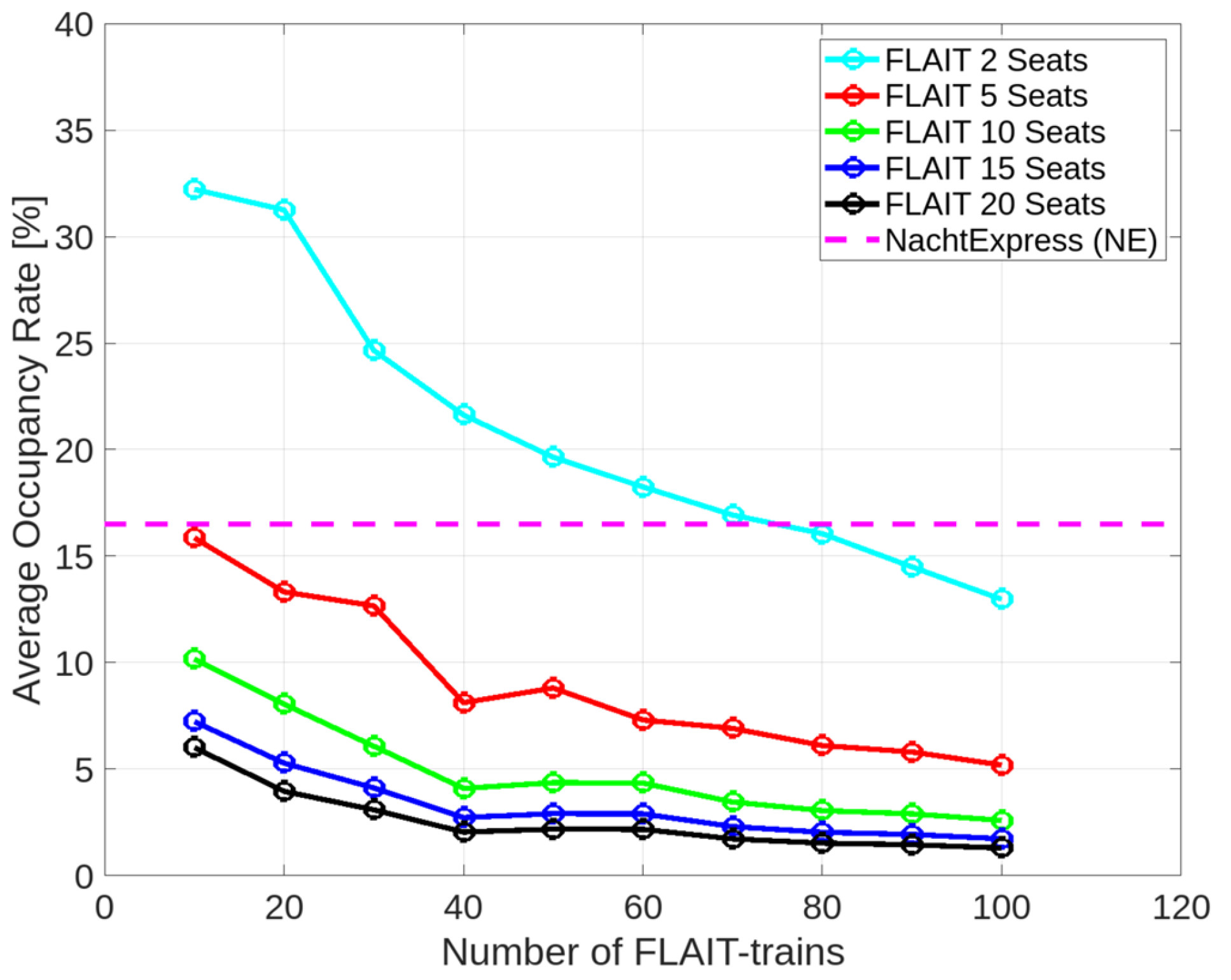
For the conventional buses, a passenger capacity (number of seating places) of 31, denoted as $C_{P,V}$, was considered according to [57]. Altogether, twelve buses were accounted for, representing the vehicle number $n_V$ for the six night bus routes. Utilizing Formula (4) with the aforementioned parameters, the average occupancy rate of the vehicles was calculated for the conventional buses, yielding a value of 16.5%.

The simulation results with FLAIT-trains, represented by the cyan line in Figure 7, demonstrate variations across different FLAIT numbers. The analysis revealed that the curve of the average occupancy rate of vehicles decreases as the number of the FLAIT-trains increases. Simulations with up to 70 FLAIT-trains exhibit a higher occupancy rate compared to the buses.

The simulation results indicate that with 10 to 70 FLAIT vehicles, the average occupancy rates of the FLAIT vehicles were higher than those of buses. Specifically, the average occupancy rates of vehicles for FLAIT-trains within this range were approximately 32.2%, 31.3%, 24.7%, 21.6%, 19.6%, and 18.2%, respectively. The improvements in the occupancy rate compared to the reference simulation were approximately 95.2%, 89.7%, 49.7%, 30.9%, 18.8%, and 10.3%.

Furthermore, with a FLAIT number between 70 and 80, the simulation results indicate that a crossover point between FLAIT-trains and buses was reached in terms of the average occupancy rate of the vehicles. For 70 FLAIT-trains, the FLAIT system’s average occupancy rate, with a value of approximately 16.9%, is still higher than that of buses by approximately 2.4%.

With 80 to 100 FLAIT-trains, the average occupancy rate of the vehicles decreased compared to the reference simulation, resulting in average occupancy rate values of 16.1%, 14.5%, and 13%, respectively.

In contrast to the reference simulation, FLAIT-trains showed disadvantages in the average occupancy rates of the vehicles, with relative decreases of 2.4% (80 FLAIT-trains), 12.1% (90 FLAIT-trains), and 21.2% (100 FLAIT-trains), respectively.

5.4.2. Exploring the Increased Passenger Capacities

The simulation results of average occupancy rate of vehicles with increased passenger capacities from 5 to 20 are incorporated into Figure 7.

The simulation results indicate a generally worse average occupancy rate of the vehicles compared to the reference simulation results. Specifically, the average occupancy rate of the vehicles decreases with increased passenger capacities. Furthermore, the average occupancy rate decreases correspondingly as the number of FLAIT-trains increases from 10 to 100. This suggests that FLAIT-trains exhibited a worse usage efficiency with the increased passenger capacities from 5 to 20. The impact of the number of FLAIT-trains and passenger capacities on the average in-vehicle time is summarized in

Table 6. Impact of passenger capacities on average occupancy rates of vehicles in [%].

	2 SPs	5 SPs	10 SPs	15 SPs	20 SPs	NE
10 FLAIT-trains	32.2	15.9	10.2	7.2	6.0	16.5
20 FLAIT-trains	31.3	13.3	8.1	5.3	4.0
30 FLAIT-trains	24.7	12.7	6.1	4.1	3.1
40 FLAIT-trains	21.6	8.1	4.1	2.7	2.0
50 FLAIT-trains	19.6	8.8	4.4	2.9	2.2
60 FLAIT-trains	18.2	7.3	4.4	2.9	2.2
70 FLAIT-trains	16.9	6.9	3.5	2.3	1.7
80 FLAIT-trains	16.1	6.1	3.1	2.0	1.5
90 FLAIT-trains	14.5	5.8	2.9	1.9	1.5
100 FLAIT-trains	13.0	5.2	2.6	1.7	1.3

.

6. Simulation Results for the On-Demand Use Cases

In the preceding sections, the simulative analysis was conducted using statistical data from the public transportation system. The available statistical data included passenger information from one bus stop to another, which was considered in the analysis. The method of simulative analysis based on statistical data proved to be suitable for the current development phase of the FLAIT-trains.

The ultimate objective of FLAIT-trains is to provide an on-demand DOOR-2-DOOR service. To address this scenario, the simulations were extended to include passenger data from the departure and arrival points, which are not limited to bus or tram stops. This required further simulative analysis for the “Night Bus Routes in Duisburg” scenario, where the transportation performance of FLAIT-trains was compared with conventional buses.

Since statistical data for the on-demand service are unavailable, some assumptions were made in this analysis. The same number of passengers was considered as in Section 5, and they were distributed randomly throughout the city of Duisburg.

In the reference simulations with conventional buses, the SUMO function “Intermodal Routing” was utilized, allowing passengers to choose between bus rides or walking as possible transport modes. This enables transfers between different night bus routes.

For simulations with FLAIT-trains, passengers were picked up directly from their departure point and transported to their destination by the FLAIT-trains. Consequently, the walking duration for passengers was reduced to zero.

Due to the functionality of “Intermodal Routing”, the quota of the walking route and time could not be ignored in the analysis. Therefore, an additional key performance figure was incorporated into this chapter alongside the ones discussed previously. The following key performance figures were considered:

• Average waiting time per passenger riding a FLAIT vehicle;
• Maximum waiting time for a single passenger riding a FLAIT vehicle;
• Average in-vehicle time per passenger riding a FLAIT vehicle;
• Average journey time per passenger.

However, due to the limitation of the available dispatch algorithm in SUMO, this paper did not conduct an analysis on the impact of the passenger capacity for each FLAIT-train.

6.1. Average Waiting Time per Passenger Riding a FLAIT Vehicle

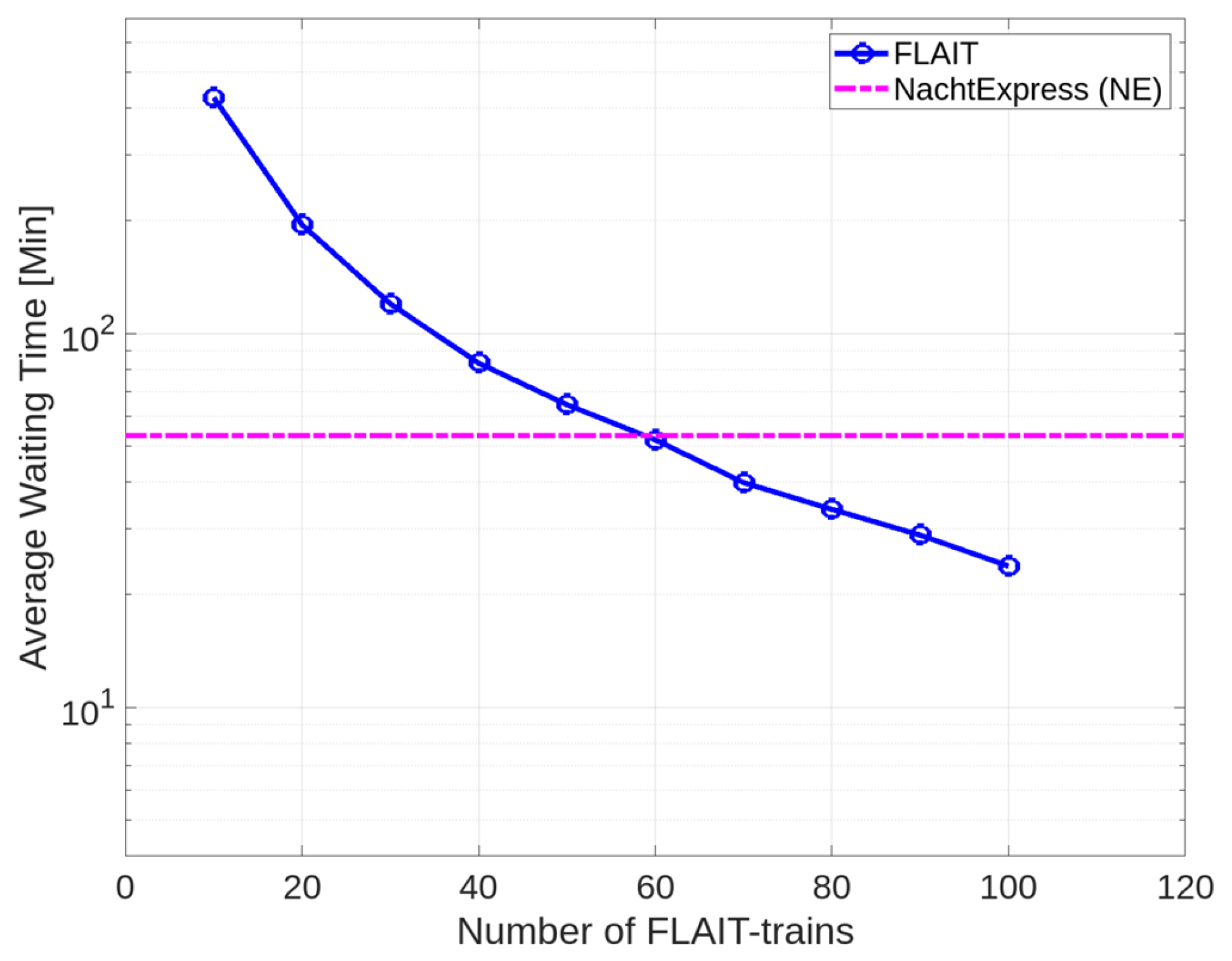
In the baseline simulations involving conventional buses, the average waiting time per passenger was determined using Equation (1), resulting in a value of 53.4 min per passenger traveling by bus.

In contrast, for FLAIT-trains, the average waiting time showed a correlation with the quantity of FLAIT-trains, as depicted in Figure 8 utilizing a logarithmic scale. Notably, the average waiting time consistently decreased with the increment in the number of FLAIT-trains.

From 10 to 50 FLAIT-Trains, the average waiting times were higher compared to the reference simulation with buses. Specifically, the average waiting times for these FLAIT-train ranges were approximately 427.3 min, 195.3 min, 120.0 min, 83.3 min, and 64.5 min. Comparatively, the average waiting times for FLAIT-trains exceeded those of conventional buses by 700.2% (10 FLAIT-trains), 265.7% (20 FLAIT-trains), 124.7% (30 FLAIT-trains), 56.0% (40 FLAIT-trains), and 20.8% (50 FLAIT-trains), respectively.

With 60 to 100 FLAIT-trains, the average waiting time decreased compared to the reference simulation, with values of 51.9 min, 39.9 min, 33.8 min, 28.9 min, and 23.9 min. FLAIT showed improvements in comparison to the reference simulation by 2.8% (60 FLAIT-trains), 25.3% (70 FLAIT-trains), 36.7% (80 FLAIT-trains), 45.9% (90 FLAIT-trains), and 55.2% (100 FLAIT-trains), respectively. The impact of the number of FLAIT-trains is summarized in

Table 7. Impact of vehicle number on the average waiting time in [min].

FLAIT Number	FLAIT	NE
10	427.3	53.4
20	195.3
30	120.0
40	83.3
50	64.5
60	51.9
70	39.9
80	33.8
90	28.9
100	23.9

.

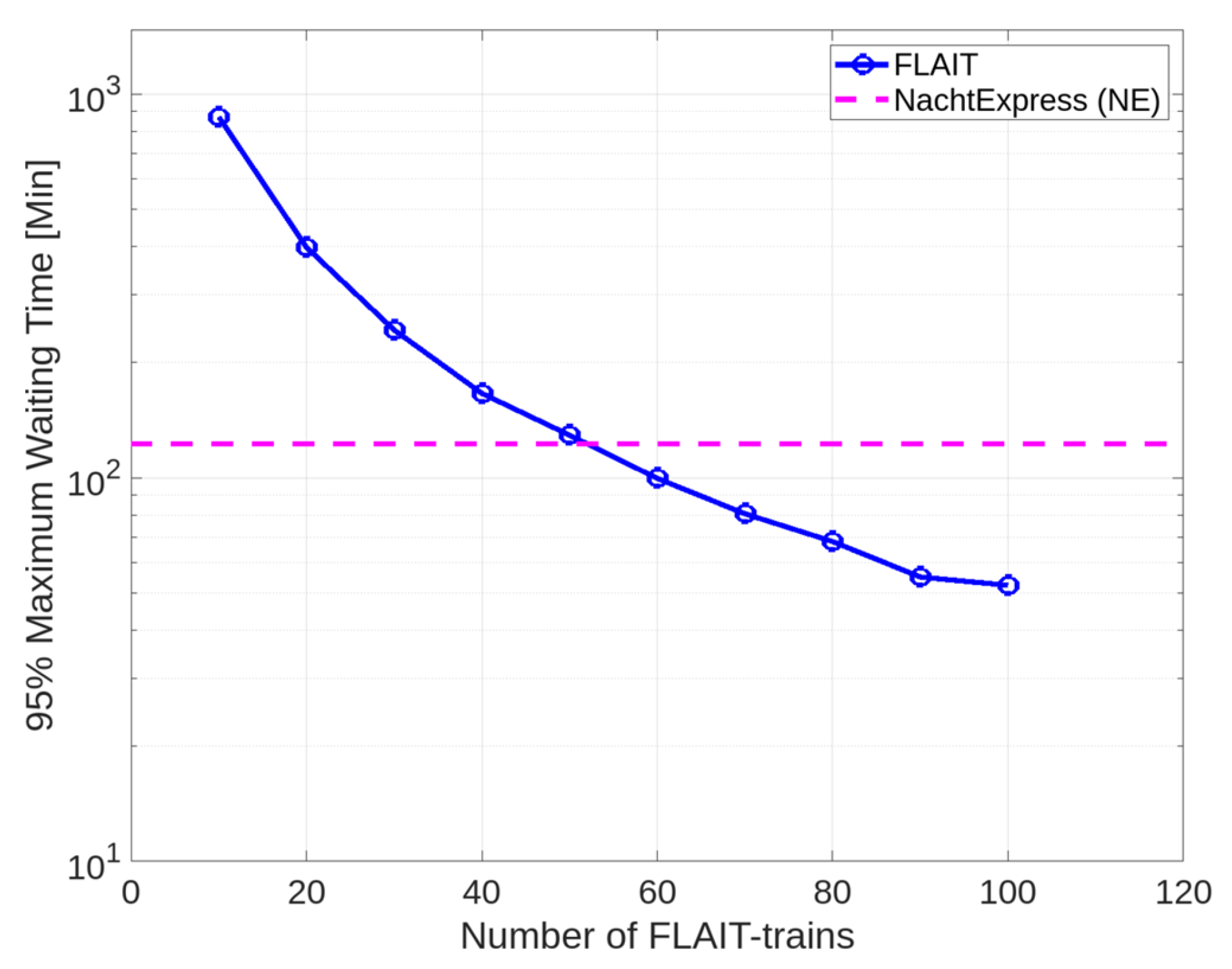
6.2. Maximum Waiting Time of a Single Passenger Riding a FLAIT Vehicle

As in Section 5.2, the 95% maximum waiting time was deemed as a more representative metric. This approach facilitated the thorough evaluation of both transportation modes, accounting for any variations introduced by the dispatching algorithm.

In the reference simulation involving night buses, the 95% maximum waiting time for a single passenger was computed using Equation (2). The simulation yielded a 95% maximum waiting time of 122.8 min for buses.

Similarly to the average waiting time, the 95% maximum waiting time for FLAIT vehicles exhibited comparable dependencies on the number of FLAIT vehicles. These dependencies are illustrated using logarithmic coordinates in Figure 9.

Between 10 and 50 FLAIT vehicles, the 95% maximum waiting times were higher compared to the reference simulation with buses. Specifically, within these FLAIT ranges, the 95% maximum waiting times were approximately 871.9 min, 398.6 min, 242.6 min, 165.9 min, and 129.1 min. When compared to the reference simulation, the 95% maximum waiting times for FLAIT-trains were longer than those of conventional buses by 610.0% (10 FLAIT-trains), 224.6% (20 FLAIT-trains), 97.6% (30 FLAIT-trains), 35.1% (40 FLAIT-trains), and 5.1% (50 FLAIT-trains), respectively.

With 60 to 100 FLAIT-trains, there was a decrease in the 95% maximum waiting time compared to the reference simulation, with values of 99.6 min, 80.5 min, 68.2 min, 55.1 min, and 52.4 min. The improvements achieved by FLAIT-trains in comparison to the reference simulation were 18.9% (60 FLAIT-trains), 34.4% (70 FLAIT-trains), 44.5% (80 FLAIT-trains), 55.1% (90 FLAIT-trains), and 57.3% (100 FLAIT-trains), respectively. The impact of the number of FLAIT-trains is summarized in

Table 8. Impact of vehicle number on the 95% maximum waiting time in [min].

FLAIT Number	FLAIT	NE
10	871.9	122.8
20	398.6
30	242.6
40	165.9
50	129.1
60	99.6
70	80.5
80	68.2
90	55.1
100	52.4

.

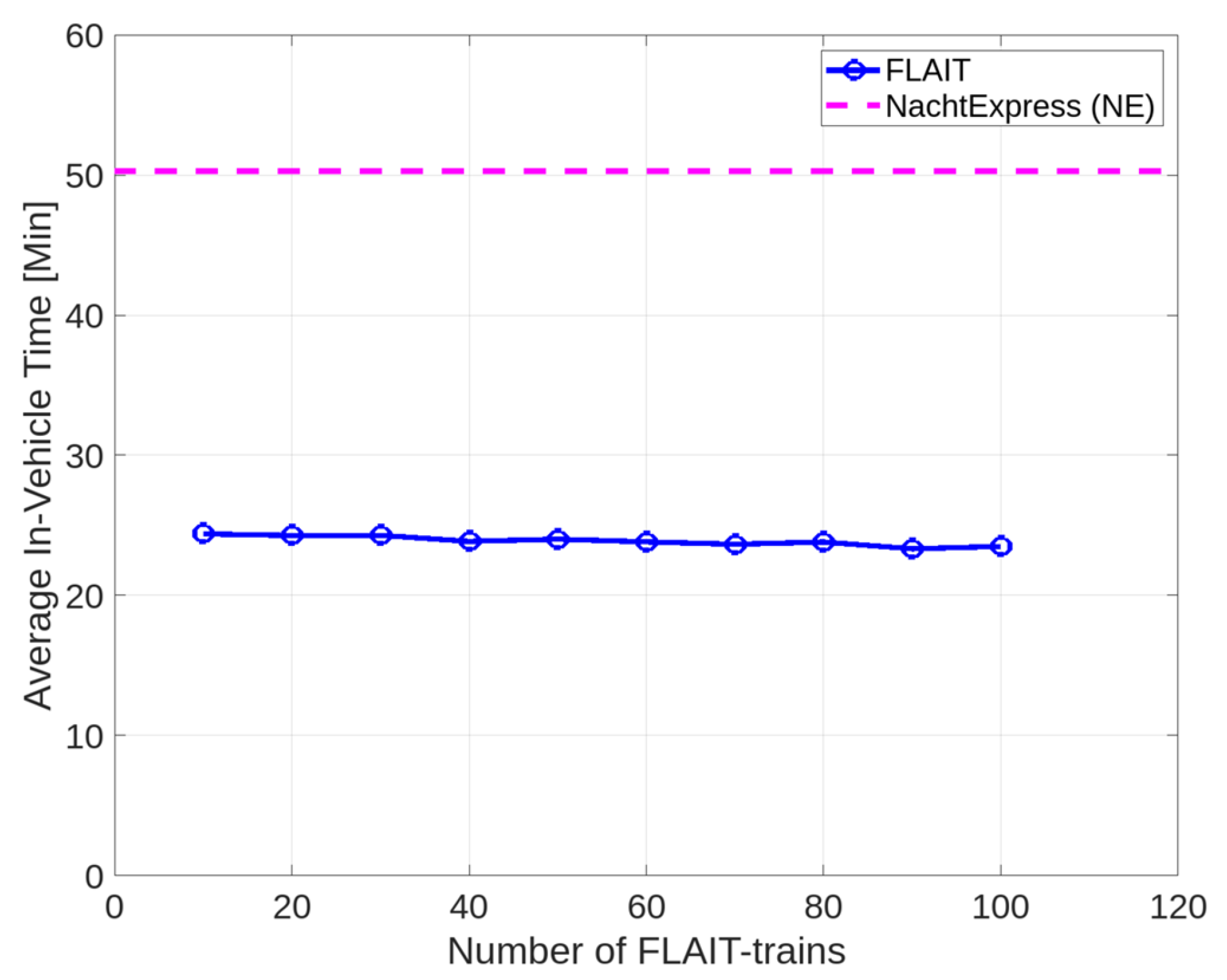
6.3. Average In-Vehicle Time per Passenger Riding a FLAIT Vehicle

The average in-vehicle time for FLAIT vehicles was found to be shorter than bus trips due to the absence of intermediate stops, as depicted in Figure 10. Using Equation (3), the average in-vehicle time per bus passenger was calculated to be approximately 50.3 min, depending on the departure and arrival points.

In comparison to the reference value from the bus simulations, the trips using 10 to 100 FLAIT vehicles took between 23.3 min and 24.4 min. The elimination of intermediate stops allowed the passengers to reduce their in-vehicle time by approximately 51.5%. The impact of the number of FLAIT vehicles on the average in-vehicle time is summarized in

Table 9. Impact of vehicle number on the average in-vehicle time in [min].

FLAIT Number	FLAIT	NE
10	24.4	50.3
20	24.3
30	24.3
40	23.9
50	24.0
60	23.8
70	23.7
80	23.8
90	23.3
100	23.5

.

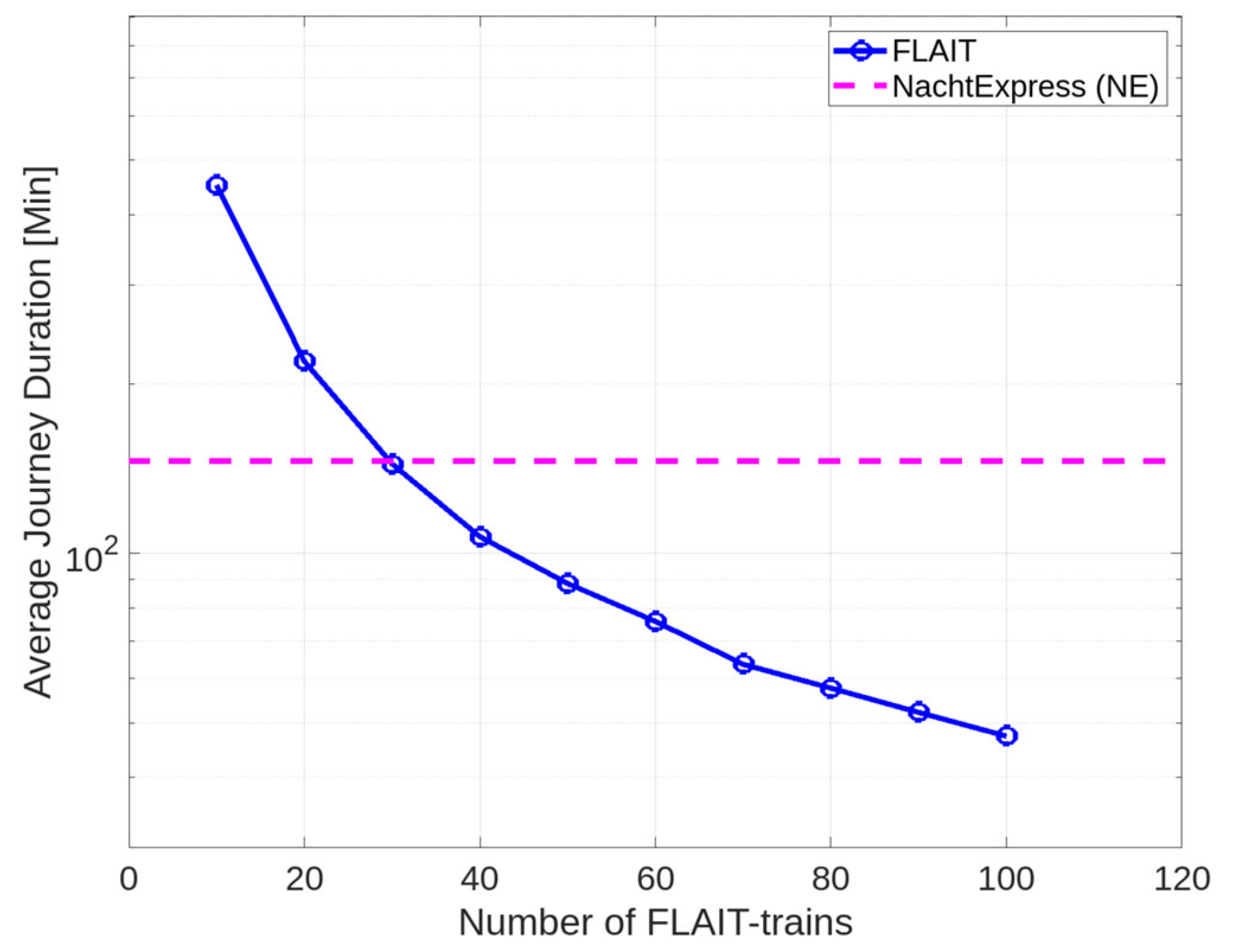
6.4. Average Journey Time per Passenger

In this on-demand service scenario, the journey time of a passenger is described as the time interval from the departure to the arrival point. In the public transportation system, a passenger could choose whether to walk to the next bus stop or opt for a longer journey to save waiting time at the bus stop. Due to the limitation of walking speed, the total journey time could increase if the passenger walks a long distance to save the waiting time at the bus stop. For this reason, the average journey time per passenger must be considered as a key performance measure, as shown in Figure 11, where the average journey time per passenger amounts approximately 146.1 min.

Similar to the average waiting time, the average journey time for FLAIT vehicles exhibited similar dependencies on the number of FLAIT vehicles. These dependencies are visualized as logarithmic coordinates in Figure 11.

For FLAIT-trains ranging from 10 to 20 units, the average journey times were higher compared to the reference simulation with buses. Specifically, the average journey times for these FLAIT ranges were approximately 451.7 min and 219.6 min, respectively. When compared to the reference simulation, the average journey time for FLAIT-trains exceeded that of conventional buses by 209.2% (10 FLAIT-trains) and 50.3% (20 FLAIT-trains).

However, with 30 to 100 FLAIT-trains, the average journey time decreased compared to the reference simulation. The journey times for these ranges were 144.3 min, 107.1 min, and 88.5 min, 75.8 min, 63.6 min, 57.7 min, 52.2 min, and 47.4 min, respectively. The improvements achieved by FLAIT-trains compared to the reference simulation were 1.2% (30 FLAIT-trains), 26.7% (40 FLAIT-trains), 39.4% (50 FLAIT-trains), 48.1% (60 FLAIT-trains), 56.5% (70 FLAIT-trains), 60.5% (80 FLAIT-trains), 64.3% (90 FLAIT-trains), and 67.6% (100 FLAIT-trains). The impact of the number of FLAIT-trains is summarized in

Table 10. Impact of vehicle number on the average journey time in [min].

FLAIT Number	FLAIT	NE
10	451.7	146.1
20	219.6
30	144.3
40	107.1
50	88.5
60	75.8
70	63.6
80	57.7
90	52.2
100	47.4

.

7. Conclusions and Outlook

In this paper, an alternative system to the conventional public transportation system was investigated and analyzed in a realistic scenario using simulations. The advantages and disadvantages of both the public transportation and FLAIT-train systems are summarized in

Table 11. Advantages and disadvantages of public transportation systems and FLAIT-trains [40].

	Public Transportation Systems	FLAIT-Train
Pros	+ Environmental friendliness + Cheaper compared to using a private car + Possibility of avoiding traffic jams + High passenger capacity	+ Environmentally friendly + Cheaper compared to using a private car + Good accessibility (without fixed stops) + Shorter waiting time + Shorter in-vehicle time + Independence of the time schedule + Better seating comfort and privacy due to low passenger numbers + Lower investment and inspection costs
Cons	− Poor accessibility to fixed stops − Long waiting time − Long in-vehicle time due to intermediate stops − Lack of passenger’s privacy and comfort − High investment costs for infrastructure − High inspection costs − Large surface area occupancy	− Large number of vehicles required due to low passenger seating capacity − Large surface area occupancy

.

In the evaluation of the “Night Bus Routes in Duisburg” scenario, some key performance measures were considered, including the average waiting time per passenger, the maximum waiting time of a single passenger, the average in-vehicle time per passenger, and the average occupancy rate of the vehicles. For the analysis of the on-demand use-case, the average journey time per passenger was considered as an additional key performance measure. To assess these measures, a realistic urban scenario was created in the SUMO simulation environment. The impact of an increased passenger capacity on the transportation performance was also investigated.

The question posed at the beginning of this paper, regarding whether FLAIT-trains are capable of replacing conventional public transportation systems, has been analyzed and answered using the simulation results. The results of the simulation based on the statistical data revealed that the transport capacity of the six existing bus routes in Duisburg could be effectively covered by 30 FLAIT vehicles with a passenger capacity of five seating places, demonstrating their superior performance if the average waiting time, the 95% maximum waiting time, and the average in-vehicle time were considered. The FLAIT-vehicles exhibit a worse performance compared to buses, if the average occupancy rate of the vehicles is considered. A comprehensive comparison of the transport capacity between buses and FLAIT-trains is presented based on the statistical data in

Table 12. Transport capacity comparison between buses and 30 FLAIT-trains in the scenario “Night Bus Routes in Duisburg” based on the statistical data.

	Buses	30 FLAIT-Trains
Average waiting time [min]	26.5	26.8
95% maximum waiting time [min]	57.9	59.4
Average in-vehicle time [min]	16.7	9.8
Average occupancy rate of vehicles [%]	16.5	12.7

.

The simulation results for the real on-demand use case indicated that the transport capacity of the current public transportation system for the night bus routes in Duisburg could be effectively met by 60 FLAIT-trains with a passenger capacity of two seating places, provided that four key performance measures were taken into account. Alternatively, if the average journey time is considered as a criterion, 30 FLAIT-trains are capable of replacing the public transportation system in this scenario. A comprehensive comparison of the transport capacity between public transportation system and FLAIT-trains is presented in

Table 13. Transport capacity comparison between public transportation system and FLAIT-trains in the scenario “Night Bus Routes in Duisburg” for on-demand use case.

	Walking + NE	30 FLAIT-Trains	60 FLAIT-Trains
Average waiting time riding by bus [min]	53.4	120.0	51.9
95% maximum waiting time riding by bus [min]	122.8	242.6	99.6
Average in-vehicle time riding by bus [min]	50.3	24.3	23.8
Average journey time [min]	146.1	144.3	75.8

.

In the FLAIT simulations conducted so far, the state of charge of the vehicle battery was not taken into account, and each FLAIT-train was assumed to operate without needing to recharge its battery. However, in future steps of the research, the battery capacity, energy consumption, and charging infrastructure (such as charging station) will be considered as the constraints in the simulations. By incorporating these factors, the exact number of FLAIT-trains required to operate efficiently in the realistic urban scenario can be determined. This additional analysis will provide valuable insights into the practical implementation and optimization of the FLAIT system for public transportation.

In this paper, the dispatching algorithm integrated in SUMO was utilized to analyze the performance of FLAIT-trains. However, it should be noted that the current dispatching algorithm only considers the average waiting time as a cost function. To further optimize the performance of FLAIT-trains and enhance their transport capacity, potential improvements can be made in the dispatching algorithm.

One potential enhancement is to include additional key figures, such as the maximum waiting time of a single passenger and average occupancy rate, in the calculation of the cost function. By incorporating these metrics, the dispatching algorithm can make more informed decisions and prioritize actions that reduce both the average and maximum waiting times for passengers. This approach can lead to a better overall transport experience for passengers using FLAIT-trains.

Furthermore, by considering the daily transportation productivity, the algorithm can focus on maximizing the efficiency of the entire transportation system rather than just optimizing individual aspects. This can lead to a more balanced and effective use of FLAIT-trains, ultimately improving their overall transport capacity and ensuring a smoother operation.

Incorporating these optimization potentials into the dispatching algorithm will contribute to a more comprehensive evaluation of the FLAIT-trains’ performance and help identify the most efficient configurations for implementing this transportation system in real-world urban scenarios.

In this paper, the Krauss model along with the perfect driver model was initially used to model flexible platooning. However, to explore and evaluate different possibilities for autonomous vehicles and their behaviors in platooning scenarios, further car-following models will be considered in future research.

One such car-following mode that will be investigated is the model specified in [58], which is specifically designed for autonomous vehicles. This model takes into account the unique characteristics and capabilities of autonomous vehicles, which may differ from conventional vehicles with human drivers. By incorporating this model into the simulation, researchers can better understand how autonomous vehicles perform in flexible platooning situations and assess their potential benefits and limitations.

By exploring different car-following models, researchers can gain a deeper insight into the behavior of vehicles in platooning scenarios, how different driving characteristics impact platooning efficiency and safety, and ultimately identify the most suitable model for the specific context and objectives of the study.

Indeed, as an intermediate solution, the FLAIT-train system addresses certain challenges conventional public transportation systems face, but some issues remain unsolved. One such problem is the large space occupancy of FLAIT-trains, which could be improved in the future to achieve fully autonomous FLAIT-trains.