Statistical and Clustering-Based Assessment of Variable Speed Limits Effects on Motorway Performance from Real-World Observations

Abstract

Variable Speed Limit (VSL) systems aimed at reducing congestion and improving safety performance have been implemented around the world in previous years. However, field studies have shown controversial results regarding traffic performance improvement. This study integrates statistical testing methods and clustering techniques for assessing the effect of a non-mandatory VSL system on traffic flow performances on a 14-km portion of the Padua–Mestre motorway in Italy. Statistical analysis is conducted on the observed speeds, collected for almost one year, to identify any significant differences provided by VSL activation. The changes in global motorway performances induced by the VSL in typical traffic patterns under recurring congestion are assessed using both statistical tests and two specific clustering algorithms, namely K-means and DBSCAN. The results indicate that the VSL system effectively affects the observed speeds and alleviates congested conditions: the observed reduction in mean travel time ranges is around 4% with the VSL system active across various lanes; the standard deviation of vehicular speeds witnessed a decrease of 12% to 20% in the most congested segments, while no notable distinction is observed in traffic flows.

1. Introduction

Variable speed limit (VSL) system is a traffic management strategy aimed at reducing congestion and improving road safety [1]. Dynamic speed control using VSL requires the use of Variable Message Signs (VMS) or the use of on-board devices communicating the suggested speed limit to the driver in this way that the system suggests lower speed limits for the upstream traffic sections and higher speeds in downstream, aiming to slow down the incoming vehicles and let the forming congestion dissolve faster. The speed limits change dynamically based on a control algorithm that can use the information about the real-time traffic conditions on the road and other variables, including weather events, visibility, traffic volumes, and accidents [2].

The main benefits identified through some real-world applications of the system include smoother journeys with more reliable travel times, reduction in the number and severity of accidents, and reduction of noise, vehicle emissions, and fuel consumption. However, other studies in the literature showed controversial results [1,2,3]. So, the conclusion on this matter is still under debate. Indeed, the success of the application of a VSL system relies both on the control algorithm, which must be robust and responsive to traffic changes, and the compliance factor, depending on the type of the system (mandatory or advisory) and the enforcement measures applied on the road.

This study takes place within a wider project concerning a dynamic traffic model for large-scale road network monitoring and control that extends the previous authors’ research [4]. Different control schemes need to be identified and optimized, based, for example, on a simulation–optimization approach [5]. This research aims to examine the impact of VSL on driver behavior and traffic flow on the Padua–Mestre expressway by assessing the distributions of the observed speeds as well as travel times, travel distances, and average speed with and without activation of the VSL system.

The study contribution consists of providing a comprehensive analysis of the operational impact of VSL using a large dataset on the Padua–Mestre motorway to provide an answer on the effectiveness of VSL in reducing traffic congestion based on data collected in the field; the impact is analyzed for different traffic conditions, including the episodes of recurrent traffic congestion, by using two different and complementary methods including consolidated statistical methods and a clustering approach.

The paper is organized as follows: Section 2 addresses the state of the art on VSL systems. Section 3 describes the methods used to analyze the data. Section 4 reports the case study and the results of the analysis performed on a portion of the Padua–Mestre expressway. Finally, a discussion of the results is addressed in Section 5, and the conclusions are reported in Section 6.

2. State of the Art

The research activity on Variable Speed Limit (VSL) systems primarily falls into two main categories: implementation and testing of control algorithms by simulation models and assessment of the performances of the control systems operating in the real world.

Development of robust and responsive models’ specifications, together with accurate calibration, are needed to achieve a good grade of representativity of the modeled system. Simulation models are frequently applied to the behavior of traffic flow with the primary objective to assess the effectiveness of different control strategies with low expenses [6,7,8,9,10,11,12,13].

The first VSL system experiments were undertaken in Germany in the late 1960s. Speed limits were set by the control staff based on observations of traffic conditions monitored by cameras. The results obtained showed a homogenization effect of the individual speeds [14]. A subsequent experiment with variable speed limits was later conducted in the Netherlands on a motorway segment of approximately 6 km [15]. The results were assessed in terms of driver acceptance and behavior, as well as the operational impact of the system. However, the differences obtained were small and, therefore, difficult to attribute to the introduction of the speed limit system. The first experiences of applying the variable speed limit in the United States of America have proved ineffective [16].

In the following years, many countries implemented the VSL system control on highways. The objectives pursued by the implementation of the VSL system concerned the general harmonization of the traffic state as well as improvements in road safety and emissions.

Field evaluation of VSL systems has been performed to assess the traffic flow performance [1,3,17,18,19,20,21,22,23,24,25,26,27,28,29], driver’s compliance [18,28,30,31], and safety [3,13,22,26,27,32]. Depending on the length of the motorway and available VSL system activation data, the effectiveness of the system is often analyzed in comparative terms of the changes involved in the flow-speed–density relations [1,17,24,33]. In studies where limited data is accessible, the evaluation has been confined to a specific section of the motorway. The comparison is conducted between two singular representations [1,3,17,23], one with the VSL in operation and the other without. Conversely, in cases where ample data is accessible, statistical testing methods are employed, benefiting from both data availability and the enhanced knowledge derived from a richer dataset [18,20,21,23,25,30]. A review of the state of the art concerning application cases as development and evaluation of control algorithms can be found in [2].

Robust schemes of effectiveness evaluation need to be applied in different locations to assess the implementation of the VSL further. The assessment of the effectiveness of the system is usually measured by estimation of the total travel time spent [3,17,18,20,23,25,27], higher percentiles of the drivers’ speed distribution [1,21,22,26,30,31,32,34,35], and the changes implied to the capacity [10,24,25,29].

The effectiveness of the implemented system depends both on the control algorithm and on the compliance level of the drivers, which is affected by the compulsoriness of the speed indications provided by the system. Table 1 covers the main methods and synthetic results obtained for both simulation evaluation and field evaluation of VSL systems. While simulation studies have widely reported benefits both in safety conditions [7,9,11,12,13,36] and traffic flow performance in the case of VSL application [6,8,9,11], according to the several experimental applications of the VSL system, the effectiveness of this control strategy remains uncertain. Despite most of the field studies concerning safety having proved VSL as an effective control strategy [27,32], the studies related to road traffic performances report controversial results. While the mechanism of congestion propagation seems to be improved in some applications [17,18,20,21,22,26,27,28,29,30,31], other studies reported increases in travel time and capacity reduction [1,9,18,22,23,26,37]. Further research attention is needed to evaluate the effectiveness of different control algorithms and schemes of drivers’ attitudes towards this control strategy.

This paper aims to add quantitative evaluation research to the framework of the VSL system impact assessment applied in the real world. The effectiveness of the system application is analyzed not only using consolidated statistical analysis techniques but also by incorporating two specific clustering methods. Based on the authors’ research, clustering techniques have not been employed to assess the impact of the VSL system.

3. Methodology

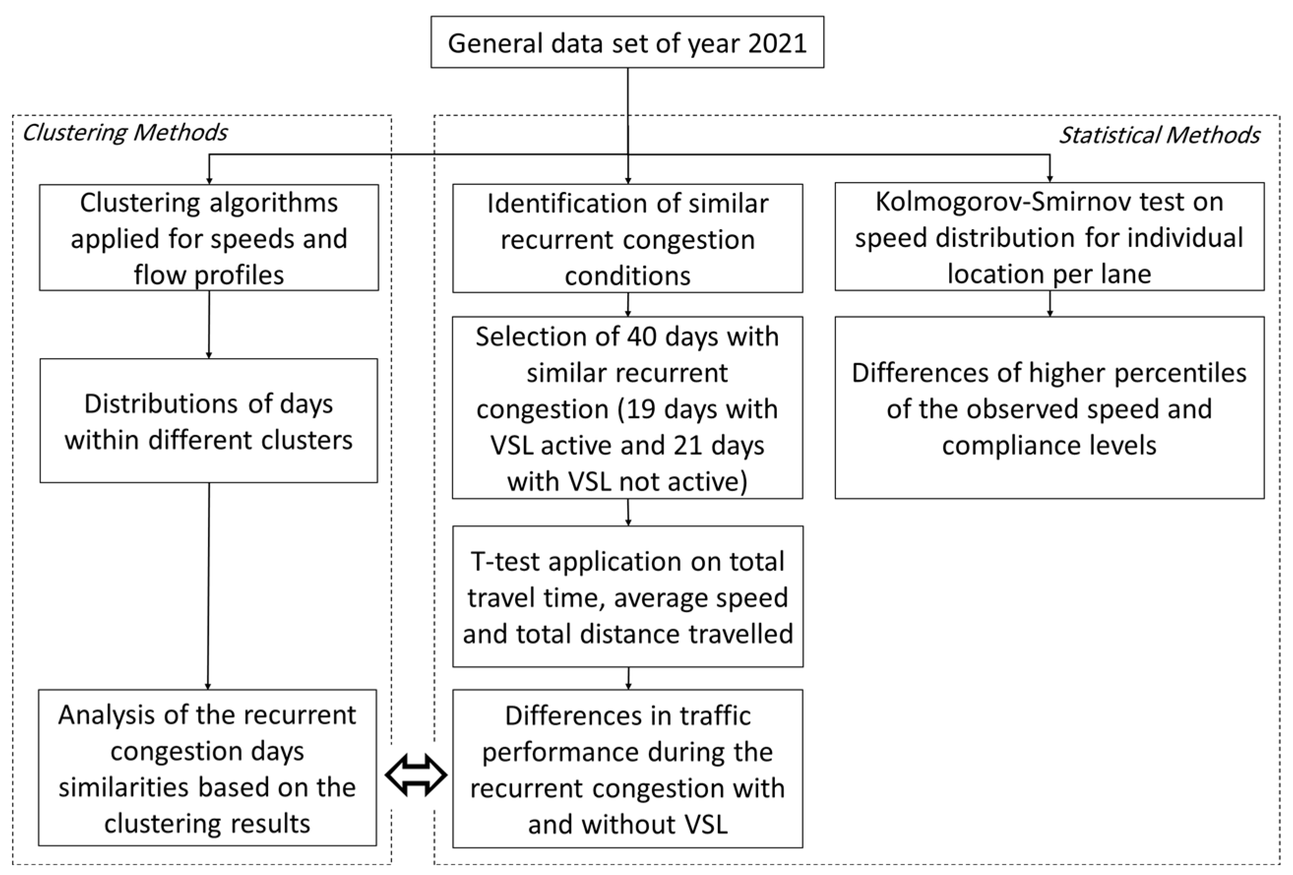
This study introduces an analysis framework that integrates data analysis statistical testing methods and clustering techniques for evaluating the effect of the VSL system on the traffic flow performance on individual lanes.

Firstly, the distributions of the observed speeds of each lane on the motorway before and after implementing VSL are compared through the statistical Kolmogorov–Smirnov test. The impact of the VSL system is then assessed by analyzing the days when recurrent congestion took place. This involves assessing total travel time, average speed, and total distance traveled using a t-test on data corresponding to periods when the VSL is active and non-active. Finally, two distinct clustering methods are applied to the observation data to reveal whether the observations with and without the VSL system pertain to the different clusters. Figure 1 summarizes the steps taken for the analysis.

Table 1. State of the art.

Location	Motorway Length (Km)	Data	Study	Assessment Measure	Evaluation Results	Ref
Barcelona	14.5	2 D 1	FE 2	Delay, emission, and safety cost function	Decrease in free flow, longer travel time, significant changes in speed distribution, general failure of VSL	[3]
Munich	18	1 D	FE	FD 3	Identification of several bottlenecks in the network and smoother flow during traffic congestion	[17]
Munich	16.3	25 DW 4, 6 DWO 4	FE	Flow Profiles	A slight decrease in capacity, congestion improvements, and notable homogeneity	[29]
Michigan	NF 5	46000 V 6	FE	Quantile regression	Significant improvement in driver compliance	[31]
Europe	NF	27 D	FE	FD	15 to 20% increase in critical density and no clear results about capacity	[1]
Seattle	11	1 D	FE	Full Bayesian analysis	Reduction of total crashes	[32]
UK	NF	1 YW 7 2 YWO 7	FE	Travel Time, Flow	Reduction in travel time and collisions	[27]
Stockholm	NF	1 DWO MW 8	FE	F-Test, FD	Not any significant impact on traffic conditions	[23]
Rotterdam	4.2	1 Y 1	FE	Traffic performance, emission, and traffic safety.	With a 3% reduction in travel time and 20% in the number of lost vehicle hours, air quality and noise levels slightly deteriorated.	[20]
Virginia	NF	23 M 1	FE	Linear regression, Z-test	Improvement in driver compliance and average speed reduction	[30]
Texas	NF	11 D	FE	Standard deviation	Improvement in flow consistency and reduction of crash severity	[22]
Missouri	61	5 D	FE	Kolmogorov–Smirnov test, FD	Change in flow–occupancy relation and decrease in average daily congestion in most locations	[21]
Virginia	20	9 M	FE	Chi-square test, Z-test	There was no increase in drivers’ compliance and a 30% reduction in travel time	[18]
Netherlands	2.2	NF	FE	FD	Improvement of traffic distribution	[28]
Barcelona	13	3 D	FE	FD	Stabilizing occupancy and preventing capacity drop	[33]
Rotterdam	3.3	2 D	FE	FD	A flow reduction of 15%	[24]
Europe	NF	14 D	FE	Mean speed	Reduction of average speed and rear-end crashes	[26]
Seattle	16	5 D	FE	t-test, TT 10, Speed	Improvement of traffic performance	[25]
Netherlands	15	149 D	FE	Shock wave speed and demand	VSL efficiency and strategy failure’s motivations	[19]
Not real	12	NF	S 9	METANET	Reduction in total travel time	[8]
Orlando	32	NF	S	PARAMICS	Safety improvement in medium-to-high-speed regimes and no benefit in low-speed situations.	[13]
Calgary	8	NF	S	PARAMICS	Safety, delay, and traffic conditions improvements	[11]
Netherlands	14	NF	S	METANET	Reduction in capacity and driver’s compliance	[10]
Edmonton	9	NF	S	VISSIM	Improved safety and mobility	[9]
Netherlands	12	5Y	S	VISSIM	Improvement in safety	[7]
Not real	2.5	NF	S	PARAMICS	Crash potential reduction and increase in travel time	[12]
Naples	6.3	NF	S	VISSIM	Improvement in mobility of network and fuel consumption	[6]
Toronto	8	6M	S	PARAMICS	Up to 50% improvement in safety and increase in travel time	[34]
Not real	21.5	NF	S	METANET	Capacity reduction	[37]

¹ D: Day, M: Month, Y: Year. ² FE: Field Evaluation. ³ FD: Fundamental Diagram. ⁴ DW: Day with VSL active, DWO: Day without VSL active. ⁵ Not Found. ⁶ Number of Vehicles. ⁷ YW: Year with VSL active, YWO: Year without VSL active. ⁸ MW: Month with VSL active. ⁹ S: Simulation. ¹⁰ TT: Travel Time.

Table 1. State of the art.

Location	Motorway Length (Km)	Data	Study	Assessment Measure	Evaluation Results	Ref
Barcelona	14.5	2 D 1	FE 2	Delay, emission, and safety cost function	Decrease in free flow, longer travel time, significant changes in speed distribution, general failure of VSL	[3]
Munich	18	1 D	FE	FD 3	Identification of several bottlenecks in the network and smoother flow during traffic congestion	[17]
Munich	16.3	25 DW 4, 6 DWO 4	FE	Flow Profiles	A slight decrease in capacity, congestion improvements, and notable homogeneity	[29]
Michigan	NF 5	46000 V 6	FE	Quantile regression	Significant improvement in driver compliance	[31]
Europe	NF	27 D	FE	FD	15 to 20% increase in critical density and no clear results about capacity	[1]
Seattle	11	1 D	FE	Full Bayesian analysis	Reduction of total crashes	[32]
UK	NF	1 YW 7 2 YWO 7	FE	Travel Time, Flow	Reduction in travel time and collisions	[27]
Stockholm	NF	1 DWO MW 8	FE	F-Test, FD	Not any significant impact on traffic conditions	[23]
Rotterdam	4.2	1 Y 1	FE	Traffic performance, emission, and traffic safety.	With a 3% reduction in travel time and 20% in the number of lost vehicle hours, air quality and noise levels slightly deteriorated.	[20]
Virginia	NF	23 M 1	FE	Linear regression, Z-test	Improvement in driver compliance and average speed reduction	[30]
Texas	NF	11 D	FE	Standard deviation	Improvement in flow consistency and reduction of crash severity	[22]
Missouri	61	5 D	FE	Kolmogorov–Smirnov test, FD	Change in flow–occupancy relation and decrease in average daily congestion in most locations	[21]
Virginia	20	9 M	FE	Chi-square test, Z-test	There was no increase in drivers’ compliance and a 30% reduction in travel time	[18]
Netherlands	2.2	NF	FE	FD	Improvement of traffic distribution	[28]
Barcelona	13	3 D	FE	FD	Stabilizing occupancy and preventing capacity drop	[33]
Rotterdam	3.3	2 D	FE	FD	A flow reduction of 15%	[24]
Europe	NF	14 D	FE	Mean speed	Reduction of average speed and rear-end crashes	[26]
Seattle	16	5 D	FE	t-test, TT 10, Speed	Improvement of traffic performance	[25]
Netherlands	15	149 D	FE	Shock wave speed and demand	VSL efficiency and strategy failure’s motivations	[19]
Not real	12	NF	S 9	METANET	Reduction in total travel time	[8]
Orlando	32	NF	S	PARAMICS	Safety improvement in medium-to-high-speed regimes and no benefit in low-speed situations.	[13]
Calgary	8	NF	S	PARAMICS	Safety, delay, and traffic conditions improvements	[11]
Netherlands	14	NF	S	METANET	Reduction in capacity and driver’s compliance	[10]
Edmonton	9	NF	S	VISSIM	Improved safety and mobility	[9]
Netherlands	12	5Y	S	VISSIM	Improvement in safety	[7]
Not real	2.5	NF	S	PARAMICS	Crash potential reduction and increase in travel time	[12]
Naples	6.3	NF	S	VISSIM	Improvement in mobility of network and fuel consumption	[6]
Toronto	8	6M	S	PARAMICS	Up to 50% improvement in safety and increase in travel time	[34]
Not real	21.5	NF	S	METANET	Capacity reduction	[37]

¹ D: Day, M: Month, Y: Year. ² FE: Field Evaluation. ³ FD: Fundamental Diagram. ⁴ DW: Day with VSL active, DWO: Day without VSL active. ⁵ Not Found. ⁶ Number of Vehicles. ⁷ YW: Year with VSL active, YWO: Year without VSL active. ⁸ MW: Month with VSL active. ⁹ S: Simulation. ¹⁰ TT: Travel Time.

3.1. Clustering of Speed and Flow Profiles

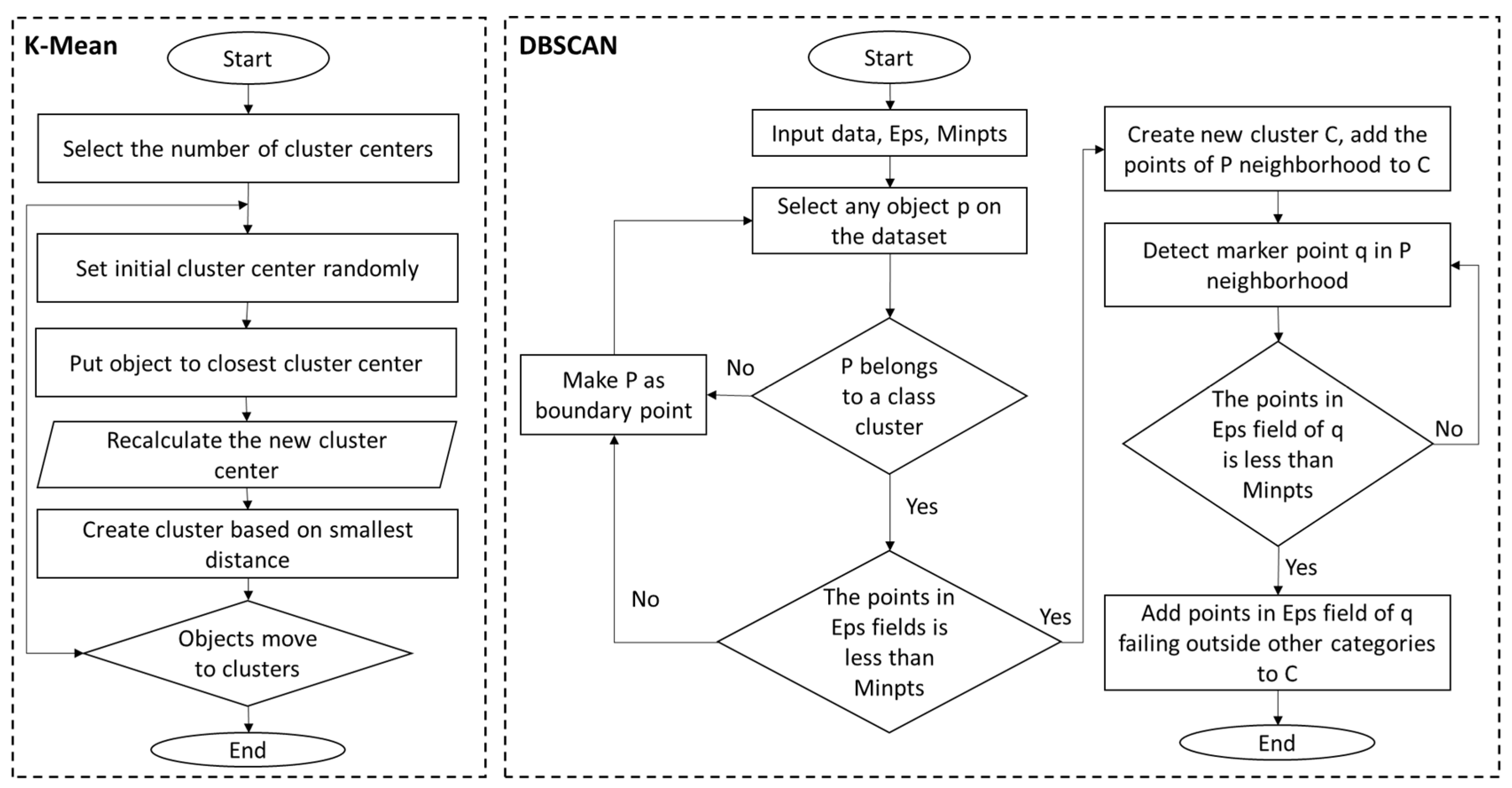
The K-means algorithm is an iterative algorithm that partitions the data into K clusters, where K is a user-defined parameter. This method aims to partition data based on their similarities. In this case, the algorithm groups the traffic speed profiles based on the Euclidean distance. The algorithm starts by randomly selecting K data points (here, speed or flow profiles) to be the initial centroids. Then, each data point is assigned to the nearest centroid based on the Euclidean distance between the data point and the centroid.

This process of assigning data points to centroids and updating the centroids is repeated until the centroids no longer change or a maximum number of iterations is reached. After the procedure convergence, each cluster contains the data points that are more like each other rather than points of other clusters.

DBSCAN (Density-Based Spatial Clustering of Applications with Noise) is a popular clustering algorithm used in machine learning and data mining to group similar data points based on their density [38]. DBSCAN is a robust clustering algorithm with broad applicability, especially in fields like pattern recognition and anomaly detection, where it can be particularly useful because of its ability to identify regions of high density in a dataset, helping to distinguish between normal and abnormal behavior. Unlike the K-Means algorithm, DBSCAN does not require the user to specify the number of clusters in advance, which makes it very useful for analyzing complex and large datasets where the number of clusters is not known beforehand. It is also relatively fast and efficient, especially for datasets with high dimensions.

The algorithm starts by selecting an unvisited point and finding all the points within a specified radius of that point, known as epsilon, which is identified using the Euclidean distance. If the number of points in the radius is greater than or equal to the specified minimum number of points, then a cluster is formed. If epsilon is set too high, then many data points that should be part of different clusters may be lumped together into one big cluster. On the other hand, if the epsilon is set too low, then some data points may be classified as noise points even though they should be part of a cluster. If the number of points is less than the minimum number of points, then the point is considered as noise or an outlier.

Once a cluster is formed, the algorithm recursively expands the cluster by finding all the points within the epsilon radius of the points in the cluster. This process continues until all the points in the cluster have been identified. The algorithm then moves to the next unvisited point and repeats the process until all points have been visited. However, DBSCAN can be sensitive to the choice of parameters, especially when the density of the data varies widely across the dataset. In such cases, it may be necessary to perform parameter tuning to achieve optimal results. Choosing a good value for epsilon often involves some trial and error and optimization methods, and in many cases, it depends on the specific dataset and the desired clustering results. Additionally, the algorithm can be computationally expensive for large datasets, as it requires calculating distances between all pairs of data points.

The elbow method is commonly used to assess the impact of input parameters on an algorithm. It is an efficient and straightforward way to identify the optimal number of clusters for K-means and the optimal epsilon value for DBSCAN. The method is based on the graphical determination of the number of clusters by indicating the “elbow” point where any further increase in the input value will not significantly improve the results. In Figure 2, the mechanism of two clustering methods is illustrated.

3.2. Statistical Tests for Traffic Performance Variables

Statistical tests are used to determine whether there is evidence to support a hypothesis, compare groups or samples, and assess the significance of differences or relationships between variables of interest. In this study, two types of statistical tests are performed:

• Student’s t-test is a statistical test used to compare the means of two independent samples or paired observations. The test is based on the t-distribution and is used when the sample size is small and the population standard deviation is unknown. The test statistic, denoted by t, is the ratio of the difference between the means to the standard error of the difference. The null hypothesis of the test is that the means of the two samples are equal. If the null hypothesis is rejected, it means that there is sufficient evidence to suggest that the means of the two samples are different.
• The Kolmogorov–Smirnov test is a non-parametric statistical method, implying no assumptions about the underlying distribution of the data, that can be used to compare the distributions of two independent samples. This test is often used when the normality assumption is not satisfied or when the shape of the distribution is unknown. The Kolmogorov–Smirnov test works by comparing the cumulative distribution functions (CDFs) of the two samples, X1 and X2. The test statistic, denoted by D, is the maximum absolute difference between the two CDFs. If the underlying distribution of X1 is shifted towards greater values than the distribution of X2, then CDF(X1) is less than CDF(X2). The p-value is the probability of obtaining a test statistic as extreme as the observed value, assuming that the null hypothesis is true. If the p-value is less than the significance level (set to 0.05 in this study), the null hypothesis is rejected, indicating that there is sufficient evidence to suggest that the samples come from two different distributions and that the distribution of X1 has higher values than the distribution of X2. It is important to note that the Kolmogorov–Smirnov test is sensitive to differences in both location and shape between the two distributions. Therefore, it can be used to detect differences that may not be detected by other tests that focus only on location (e.g., t-test).

4. Experimental Analysis

4.1. Case Study and Available Data

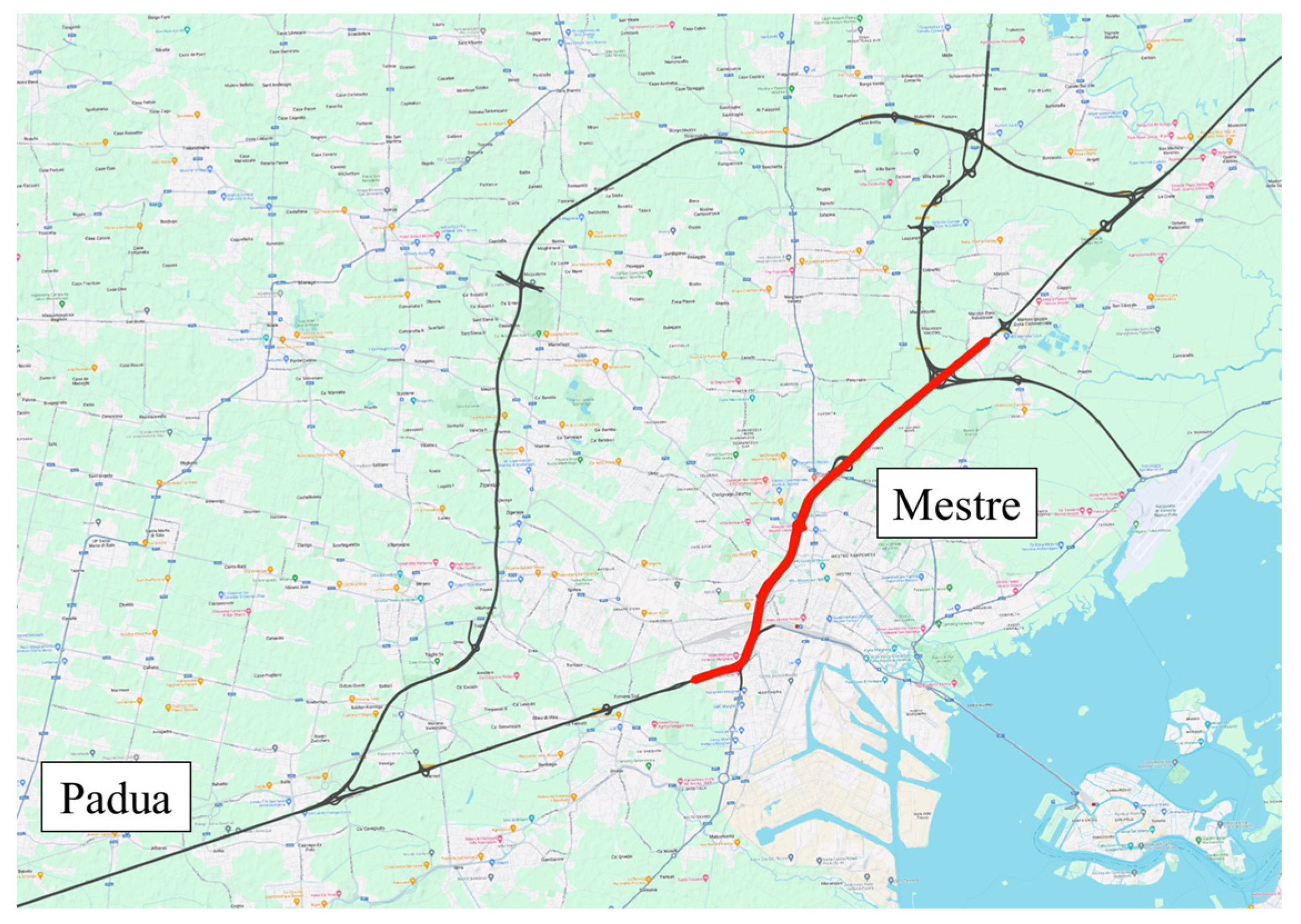
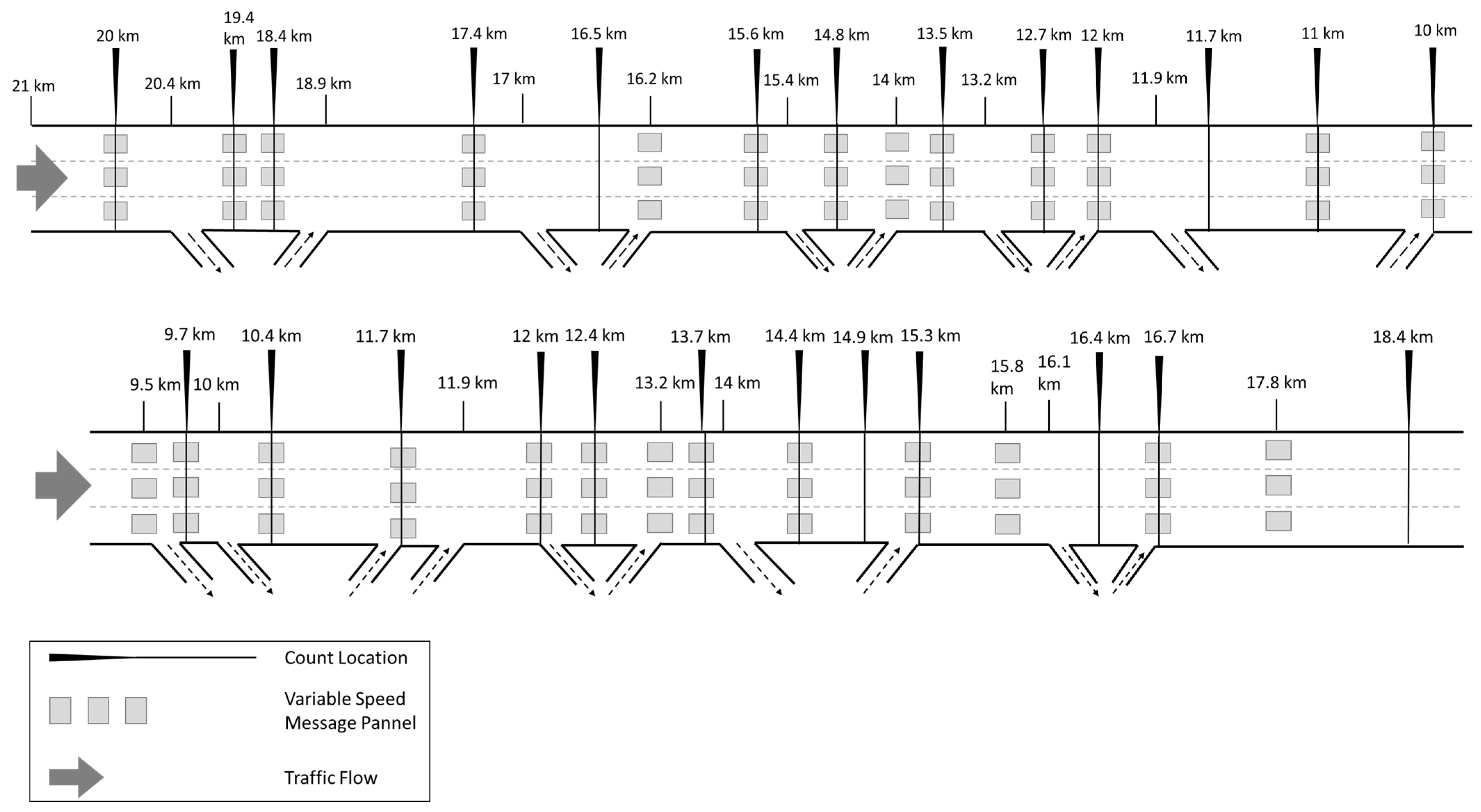
The study area is a portion of the Italian Expressway connecting Padua and Mestre cities in Figure 3; two carriageway layouts containing 10 on-ramps and 10 off-ramps are depicted in Figure 4. The length of the portion of the analyzed expressway is about 10 km. On each carriageway, 13 VMSs suggest speed limits, and several additional message signs warning of adverse weather events, accidents, and road closures are located. There are 13 count locations on each carriageway, equipped near the message signs, represented by video cameras, collecting the number of vehicles and their speed, distinguished by classes of length.

The available data used in this study included:

• a dataset relative to the state of the variable message signs.
• a dataset provided by the traffic count locations.

Every VMS shows a message sign for each lane. The dataset of the VMS reports for each message sign the timestamp and the message shown during the period from January 2021 to December 2021 for a total of 246 days of the activation of the system in different locations. The VSL system is triggered by density values exceeding critical thresholds and imposes a speed limit following rules explained in Section 4.2. Additionally, there were periods when the system was not active, and no message was shown at all. These periods did not depend on traffic conditions, so situations with different ranges of flow and speed values were observed in both the case of VSL activated and those without VSL.

The sub-dataset used for this research was limited to situations with no lane closures on the network. The analyzed traffic situations include both periods when the VSL was active and displaying a message for the three lanes and when it was not active at all.

The data collected by the count locations refer to the period from January 2021 to November 2021. The data are differentiated by light and heavy vehicles for each lane and include the traffic counts, the average arithmetic speed, the average harmonic speed, and the headway measures collected every minute. For each lane, the occupancy measure is provided together with the accuracy index for the collected data.

4.2. VSL Control Algorithm

The implemented VSL system is an advisory system without enforcement measures applied to guarantee drivers’ compliance. The control algorithm used by the Variable Speed Limit system applies 40 km/h, 50 km/h, 60 km/h, 70 km/h, 80 km/h, and 90 km/h speed limit for each lane based on the traffic conditions detected upstream.

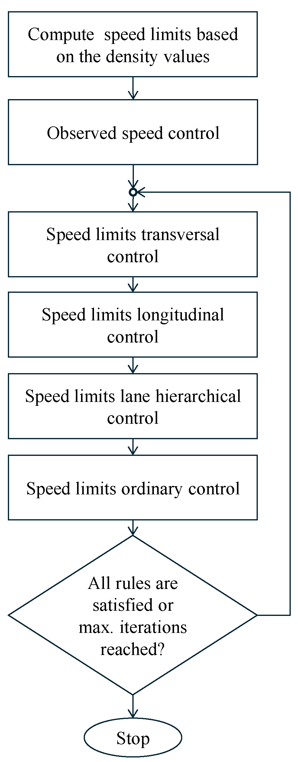
A flowchart of the control logic is reported in Figure 5. In case the observed density exceeds a threshold, defined as the critical value, a new speed limit is computed for the message signs upstream at the critical point. The estimation is achieved by computing the number of cumulated vehicles, using the observed density values, and evaluating the time necessary to discharge these cumulated vehicles. Thereafter, the speed limit is derived proportionally to the discharge time, with the aim of slowing down the incoming vehicles.

Additional steps of the control algorithm concern restraining the difference between the speed limit and the speed observed near the VMS (observed speed control), obtaining a smooth speed limit profile for sequential VMS locations (speed limits transversal control), obtaining the same values for at least two lanes (longitudinal control), and avoiding higher speed limits for slower lanes (hierarchical control), and consistency with ordinary speed limits (ordinary control).

The control algorithm operates iteratively, aiming to ensure that the rules are satisfied and that the differences stay within given thresholds.

When the system is not active the ordinary speed limit (No VSL) in the urban expressway under study is to be considered, which is equal to 90 km/h for the left and the center lanes, while the ordinary limit for the right lane, which is narrower than the standard is 60 km/h.

4.3. Motorway Performance with and without Activation of the VSL System

4.3.1. Activated Messages and Speed Limits

Generally, the analyzed cases concern the speed distributions when the VMS displayed speed limits from 40 km/h to 90 km/h. In the case of the application of a 90 km/h speed limit by the VSL system for the left lane and the center lane and the application of a speed limit of 60 km/h for the right lane, formally, there was no change imposed on the drivers with respect to the conditions when the system was not operating. However, in the case of the active VSL system, the message signs displayed the speed limits, while in the case of the inactive system, no message sign appeared on the display.

4.3.2. Analysis of the Observed Speeds with Different Speed Limits Displayed

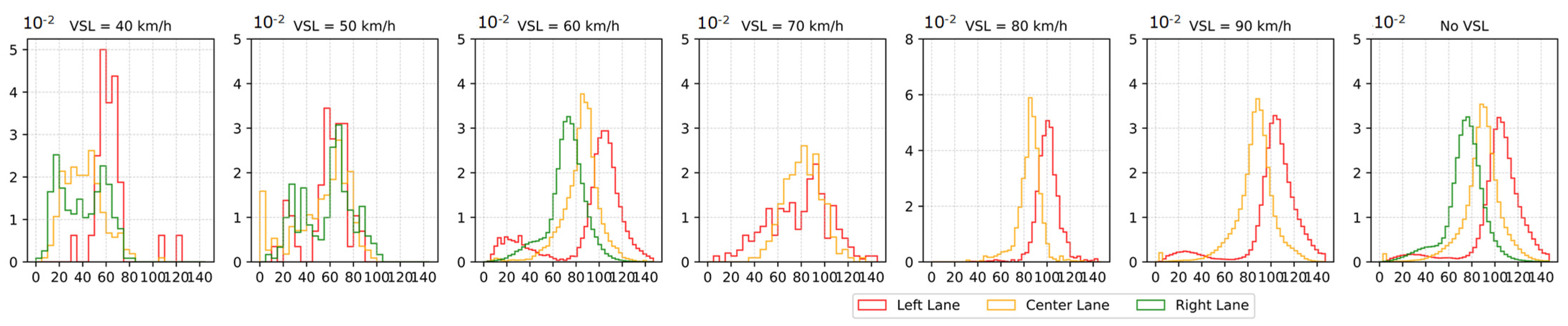
Figure 6 reports the frequency of observed speed distributions over all the available count locations for different speed limits for the three lanes. The right lane does not provide data for variable speed limits higher than 60 km/h, as its maximum speed limit is set at 60 km/h.

The distribution of the observed speed always assumes the highest values for the left lane, followed by the center lane and finally, the right lane is the slowest. In cases of No VSL applied, and the cases of 60 km/h and 90 km/h the distributions of the speeds on the left lane and on the right lane follow a bi-modal shape, indicating situations of congestion reported for some of the count locations.

In the case of the 80 km/h speed limit, the distribution of the observed speeds does not preserve such a bi-modal shape. This is because the application of this speed limit was limited itself and included only cases of forming congestion, while the limits of 90 km/h and 60 km/h were applied by the system more frequently and covered different observations of the traffic state. The application of the speed limits of 40 km/h, 50 km/h, and 70 km/h had seen only a few cases of application; for this reason, the frequency distributions do not show a smoothed shape.

As some locations report congested traffic states and the differences between observed values are moderate, the Kolmogorov–Smirnov two-sample test was conducted individually for each count location to verify whether the observed speed distributions are significantly different and are shifted towards smaller values in the case of the active VSL system.

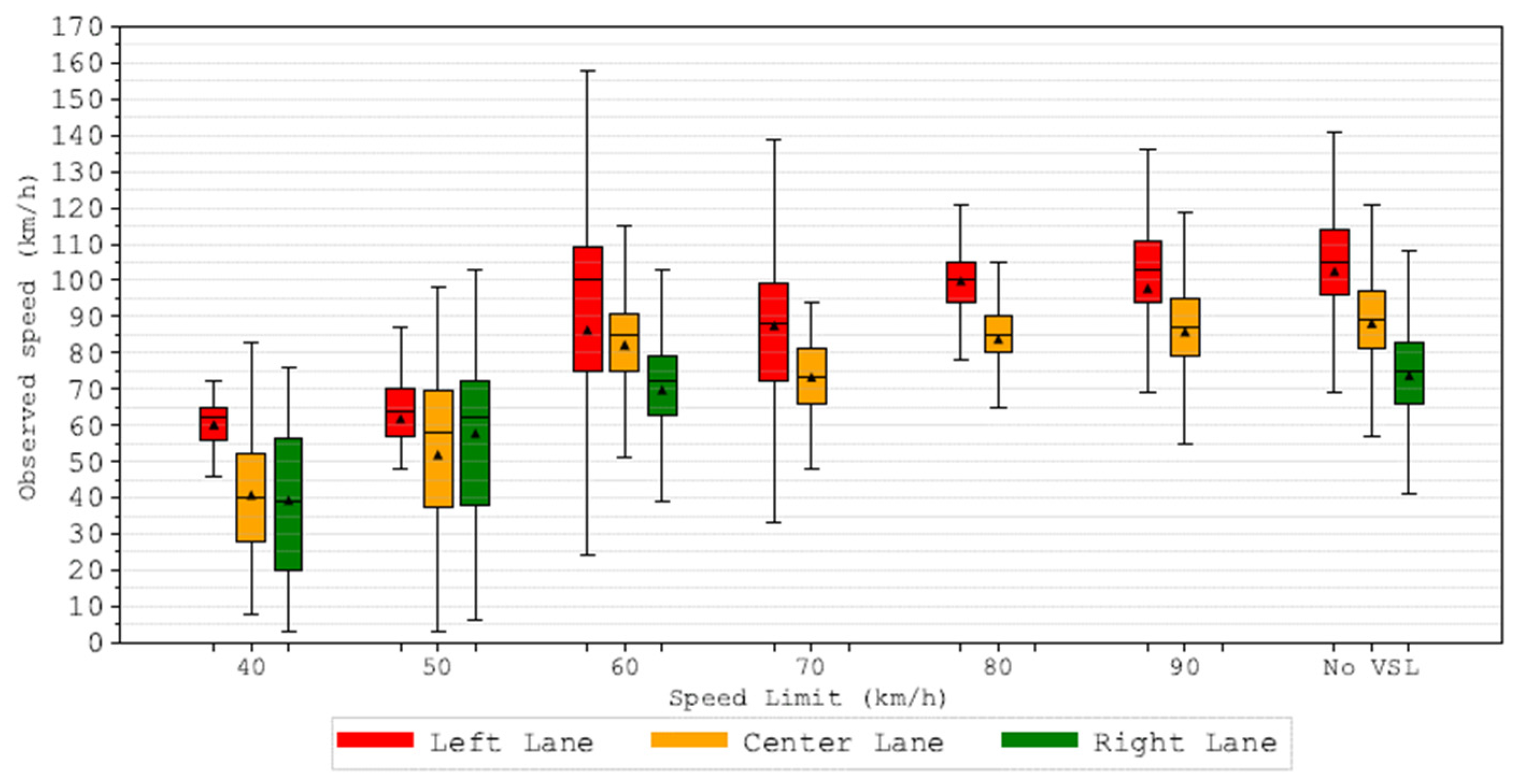
Figure 7 reports a summary of the distributions of the observed speeds on different lanes with different speed limits active, whose p-value was less than 0.05 and therefore differed significantly from the No VSL case. In each case, the first and the last quartiles are indicated by the extension of the boxes, while the median value is indicated by the black horizontal line, and the maximum and minimum values are reported by the black vertical lines. Lower values of the observed speeds correspond to lower speed limits, and the dispersion of the observed data is highest in the cases of No VSL and the speed limits of 90 km/h and 60 km/h, where many situations of congestion identified by low-speed values were observed.

The summary of the numerical results, relative to the count locations that provided significant results (p < 0.05) for the K-S test, is reported in

Table 2. Summary of K-S test applied for different count locations.

Lane	Lim	Compliance	85th Percentile	90th Percentile	95th Percentile	D85th Percentile	D90th Percentile	D95th Percentile	N Count Locations	N Count Locations (p < 0.05)
Left	No VSL	10%	119	122	128				27
Left	90	12%	113	115	119	2	3	4	27	19
Left	80	4%	107	109	111	10	11	14	24	18
Left	70	16%	102	105	108	12	11	14	8	6
Left	60	14%	105	108	113	4	5	6	21	11
Left	50	18%	69	70	72	44	46	49	5	4
Left	40	3%	66	67	68	47	49	53	4	3
Center	No VSL	45%	103	106	112				27
Center	90	53%	98	100	104	4	5	7	27	25
Center	80	30%	88	89	91	11	13	17	24	17
Center	70	18%	83	84	85	13	15	19	8	5
Center	60	6%	93	96	100	8	8	10	27	21
Center	50	16%	70	74	77	25	24	28	6	5
Center	40	33%	63	65	70	30	32	34	5	4
Right	No VSL	9%	87	90	96				27
Right	60	13%	82	84	89	3	4	5	27	22
Right	50	25%	68	71	75	13	14	19	7	5
Right	40	30%	54	56	58	22	24	31	6	4

. The statistical significance was achieved on average for 71%, 78%, and 73% of the total count locations, respectively, for the left lane, the center lane, and the right lane. As the applied speed limit decreases, the observed speed values decrease as well. In terms of the 85th percentile of the observed speeds, a reduction of 47 km/h is observed for the left lane, where the 85th percentile passes from 113 km/h in the case of a 90 km/h speed limit to 66 km/h for the speed limit of 40 km/h, while the decrease for the center and the left lane is, respectively, 30 km/h and 22 km/h.

It is also worth noting that in the case of the ordinary speed limit shown by the system, the observed speeds are significantly lower than in the case when the VSL system was not showing any message. Showing the ordinary limit by the VSL system led to a moderate reduction of the speed between 2 km/h and 4 km/h for different lanes.

As per compliance, the results show that the application of the VSL system generally increased the percentage of values below the posted speed limit. Despite the levels of compliance being moderate, the activated VSL system increased the percentage of drivers that follow the speed limit, even when an ordinary speed limit of 90 km/h for the fast lanes or 60 km/h for the right lane was displayed by the system with respect to the days when the system was not activated. For the left lane, the compliance ranged between 12% and 18% for different speed limits, except for lower compliance values of 4% and 3% that were observed, respectively, for the speed limits of 80 km/h and 40 km/h. For the center lane, the compliance ranged between 16% and 53% for different speed limits, with an exception for the speed limit of 60 km/h, when the compliance was 6%, while for the right lane, the compliance ranged between 13% and 30%. Lower compliance levels can be attributed to more fluid traffic states, where the drivers did not perceive the necessity to adjust the speed.

4.4. Motorway Performance during Recurring Congestion

One of the main objectives of the VSL system is the prevention of congestion, so further analysis focuses on recurrent congestion conditions. A visual analysis of the observed speed values on the motorway indicated that recurrent congestion took place in the same area (that is, from km 11.0 to km 13.4 on the direction from Mestre to Padua) in 40 days, relative to 19 days in which the VSL system was operating and was triggered by high-density values observed upstream, while the remaining 21 days report data when the VSL system was not operating. Statistical t-tests performed on each count location section showed that the traffic flows could be considered similar at a 5% significance level for the two observation periods.

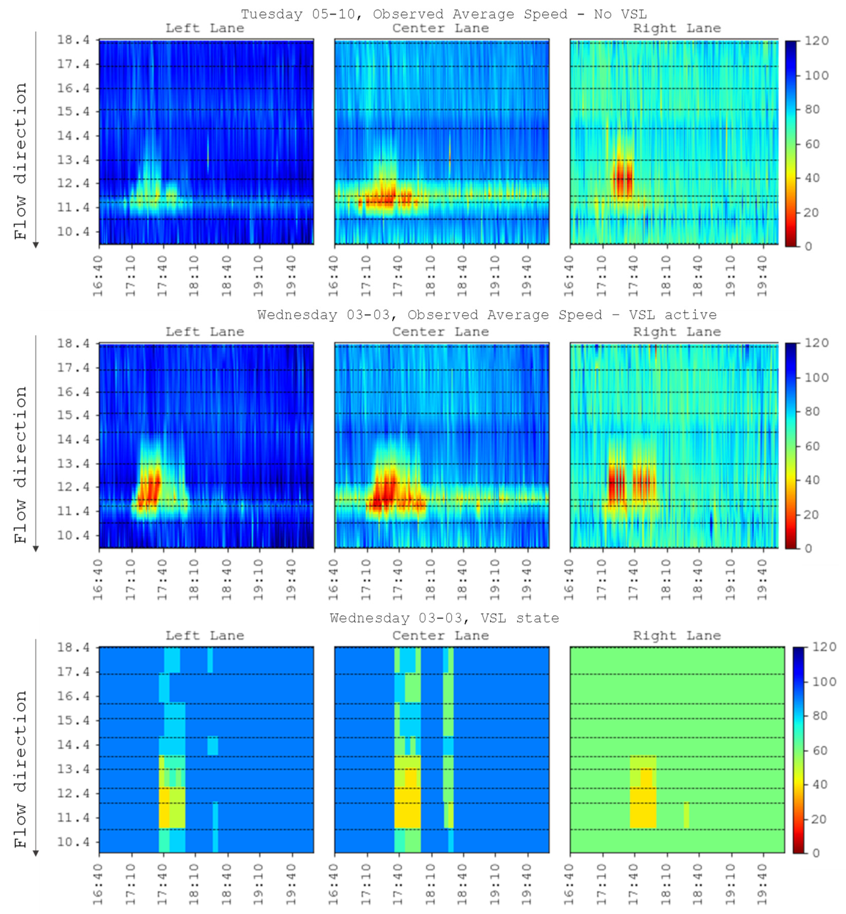
As a reference of the observed congestion in the 40 days, Figure 8 reports the heatmaps of the average observed speed per lane for the two days and a heatmap of the VSL states corresponding to the day when the system was operating; the higher values are highlighted by blue colors while the cells with lower values are individuated by yellow and red colors, for the segments between the count locations linear data interpolation was adopted to construct the relevant profiles.

On both days, the congestion started forming at around 17:10 and was dissolved at around 18:00. The figure on the top is relative to the 5 October 2021, a day when the variable speed limit system was not active, while the figure on the bottom is relative to the 3 March 2021, when the system was active and changed the speed limit shown based on the revealed conditions.

The three indicators chosen as metrics of congestion are the average speed (V avg), the mean travel time per vehicle (MTT), and the mean traveled distance per vehicle (MTD). The mean traffic flow (MQ) observed by the count locations is also computed as a reference of the observed traffic conditions.

$$V_{avg}=\frac{{\sum }_{i=1}^T{\sum }_{j=1}^N{k}_j^i{v}_j^i{l}_j}{{\sum }_{i=1}^T{\sum }_{j=1}^N{k}_j^i{l}_j}$$

$$MTT=\frac{{\sum }_{i=1}^T{\sum }_{j=1}^N{k}_j^i{l}_j{\Delta }_t}{\frac{1}{N}{\sum }_{i=1}^T{\sum }_{j=1}^N{k}_j^i{v}_j^i{\Delta }_t}$$

$$MDT=\frac{{\sum }_{i=1}^T{\sum }_{j=1}^N{q}_j^i{l}_j{\Delta }_t}{\frac{1}{N}{\sum }_{i=1}^T{\sum }_{j=1}^N{q}_j^i{\Delta }_t}$$

$$MQ=\frac{1}{NT}\sum _{i=1}^T\sum _{j=1}^N{q}_j^i{\Delta }_t$$

where $k_j^i$ and $v_j^i$ are, respectively, density and speed observed on the segment j during the time interval i, $l_j$ is the length of the segment j, and ${∆}_t$ is the time interval of data aggregation. N is the number of count sections, and T is the duration of the observation interval.

The Student’s t-test was applied to compare the values of the three indicators estimated on the sample of 19 days with the VSL system active (VSL) and on the sample of 21 days when the system was not operating (No VSL). The statistical analysis was limited to the same time duration of 200 min and the same 11 count locations with available data. The summary of the statistical analysis is reported in

Table 3. Summary of Student’s t-test applied for four indicators: average speed, V_avg; mean traveled time per vehicle, MTT; mean traveled distance per vehicle, MTD; and mean flow in the observation period, MQ. The critical value of t corresponding to a 0.05 significance level was 2.02. The significant results are highlighted in bold.

Measure	Unit	Lane	VSL State	Average	Std Dev	Difference between Average Values (VSL–No VSL)		t
V avg	[km/h]	Left	No VSL	95.7	3.7	3.1	3%	2.73
			VSL	98.7	3.4
		Center	No VSL	78.3	3.6	3.5	4%	3.69
			VSL	81.8	2.1
		Right	No VSL	69.3	2.2	3.4	5%	3.92
			VSL	72.6	3.1
		Carriageway	No VSL	83.0	2.9	3.0	4%	3.53
			VSL	86.0	2.5
MTT	[min/veh]	Left	No VSL	5.30	0.183	−0.19	−4%	−3.19
			VSL	5.11	0.195
		Center	No VSL	6.53	0.198	−0.27	−4%	−3.47
			VSL	6.26	0.283
		Right	No VSL	7.44	0.378	−0.31	−4%	−3.10
			VSL	7.12	0.234
		Carriageway	No VSL	6.24	0.199	−0.22	−4%	−3.40
			VSL	6.02	0.218
MTD	[km/veh]	Left	No VSL	8.44	0.081	−0.04	−1%	−2.11
			VSL	8.40	0.046
		Center	No VSL	8.51	0.039	0.01	0%	0.63
			VSL	8.52	0.032
		Right	No VSL	8.57	0.078	0.05	1%	1.86
			VSL	8.62	0.091
		Carriageway	No VSL	8.50	0.022	0.00	0%	−0.21
			VSL	8.49	0.027
MQ	[veh/h]	Left	No VSL	1025	109	−16	−2%	−0.43
			VSL	1009	132
		Center	No VSL	1396	36	−12	−1%	−0.46
			VSL	1384	112
		Right	No VSL	601	14	−15	−3%	−1.38
			VSL	585	49
		Carriageway	No VSL	3022	142	−62	−2%	−1.15
			VSL	2959	199

.

Statistically significant results were observed for all three lanes for the average speed and the mean travel time. On the days with the VSL system activated, higher speeds were observed for the three lanes, and the differences were 3.1 km/h (3%), 3.5 km/h (4%), and 3.4 km/h (5%), respectively, for the left, central, and right lanes.

With reference to a 1-km long segment, the MTT obviously equals the inverse of the average speed; however, it is useful to report it with reference to the average distance traveled by the drivers on the motorway stretch under analysis. In fact, with VSL activated, the average travel time on the carriageway was 6.02 min, with a 4% reduction with respect to the average travel time without VSL (6.24 min). The mean travel time was reduced on the days when the VSL was active; the reduction was 0.19 min (−4%), 0.27 min (−4%), and 0.31 min (−4%), respectively, for the left, central, and right lanes.

The results for the mean distance traveled are similar for the two observation periods. For the left lane, the mean distance traveled was slightly reduced by 0.04 km (−1%) on the days when the system was operating, and the statistical significance was reached, while for the remaining two lanes, the mean traveled distance was slightly higher when the system was operating, and the results are not statistically significant. Since the flows on the ramps are not directly observed, the slight difference observed in the mean traveled distance can be attributed to variation in demand patterns. The mean flows were slightly lower on the days when the system was operating (reduction between 1% and 2% for the different lanes) and showed significant similarity in the two observation periods.

4.5. Clustering Analysis Results

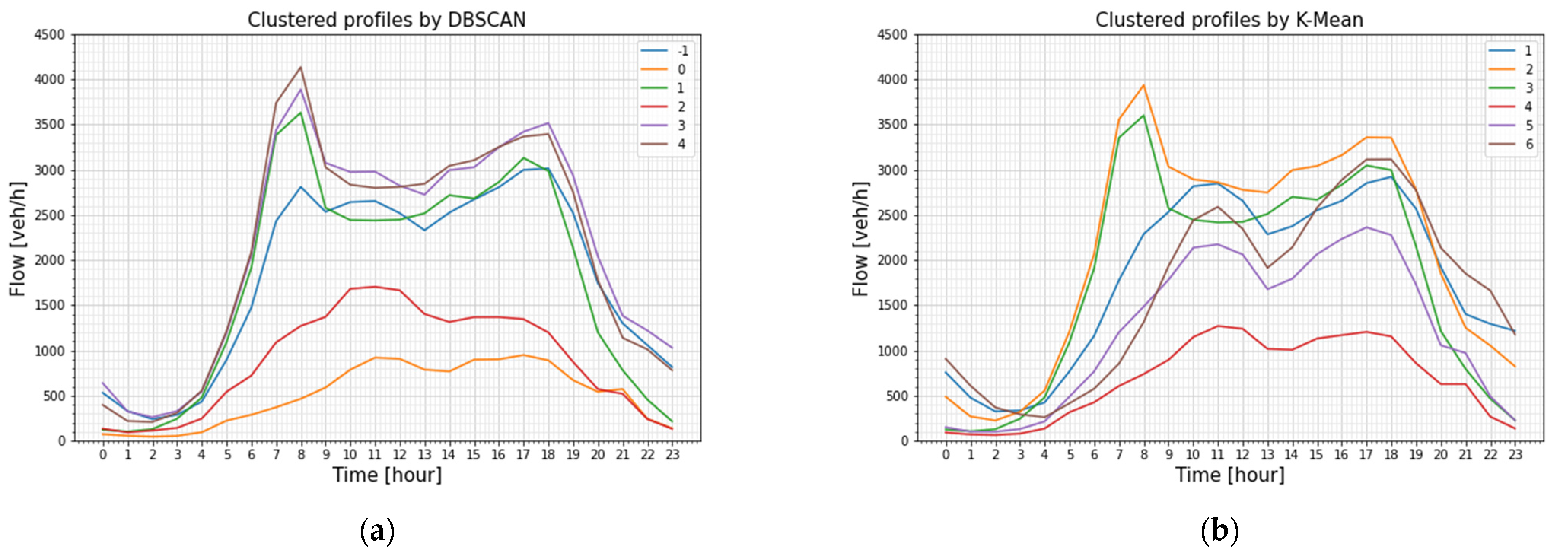
The K-Means and DBSCAN clustering algorithms were applied both for the flows and speed profiles for each count location separately to derive the traffic behavior patterns. The results are analyzed by considering the distributions of the number of days assigned to different clusters, with a further focus on the recurrent congestion and the state of the VSL system. Scikit-learn Python’s library was used to implement the clustering analysis.

Six clusters were found to be suitable by the Elbow method, applied for clustering of the flow profiles by the K-Means algorithm. The DBSCAN algorithm has distinct input value definitions for speed profile clustering and flow profile clustering. The epsilon parameter sets the limit for the greatest distance that a data point can have from a previously visited point, or else it will be treated as an outlier. To find the optimal epsilon value for each clustering method, the Elbow method was employed to minimize the sum of squared distances of points within each cluster. The found epsilon value was 20 for the speed profiles, while for the flow profiles, the epsilon value was 500. An example of flow clustering results shown in Figure 9 provides a comparison between how two algorithms grouped traffic profiles for one section and displays substantially different clusters aligning with expected transportation patterns.

The K-Means algorithm performed clustering by dividing the data into distinct clusters based on the weekdays, Sundays, and Saturdays for both the school period and summer, while the DBSCAN provided three distinct yet similar clusters.

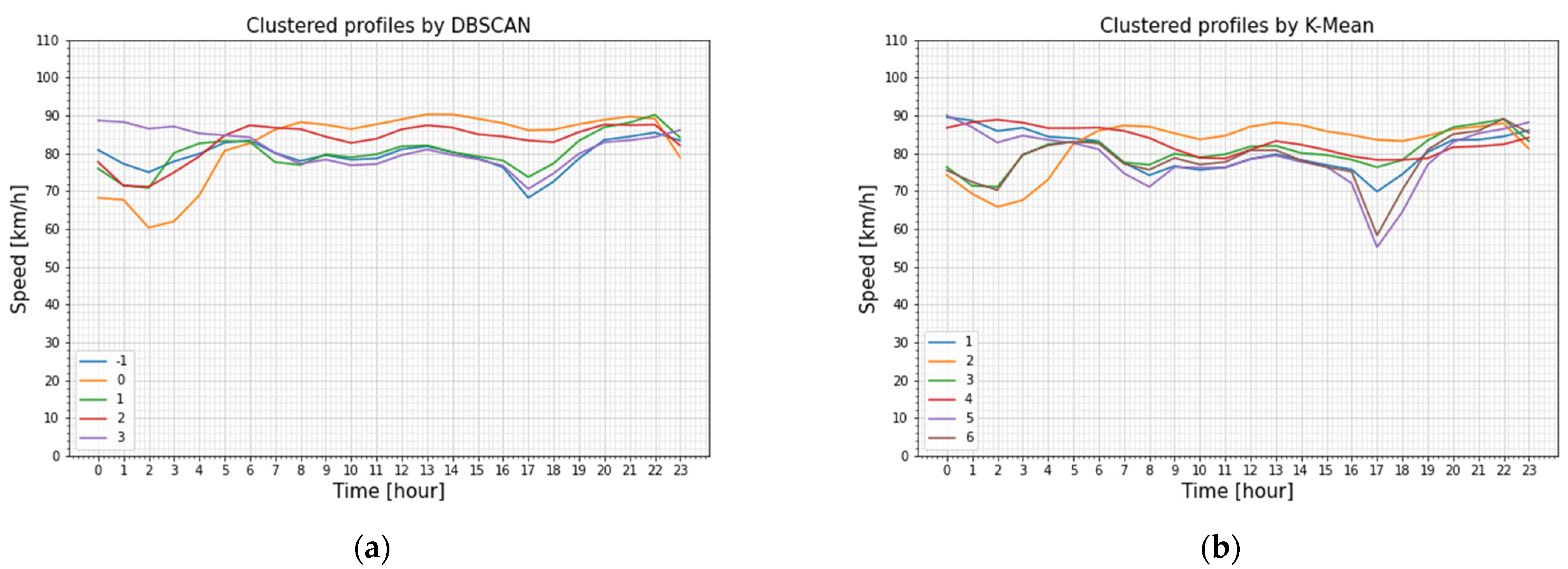
As for the clustering of the speed profiles, DBSCAN provided on average three clusters for each detector. Figure 10 illustrates an example of the clusters obtained for the speed profiles, where both algorithms identified significant differences in the congestion peak in the morning hours.

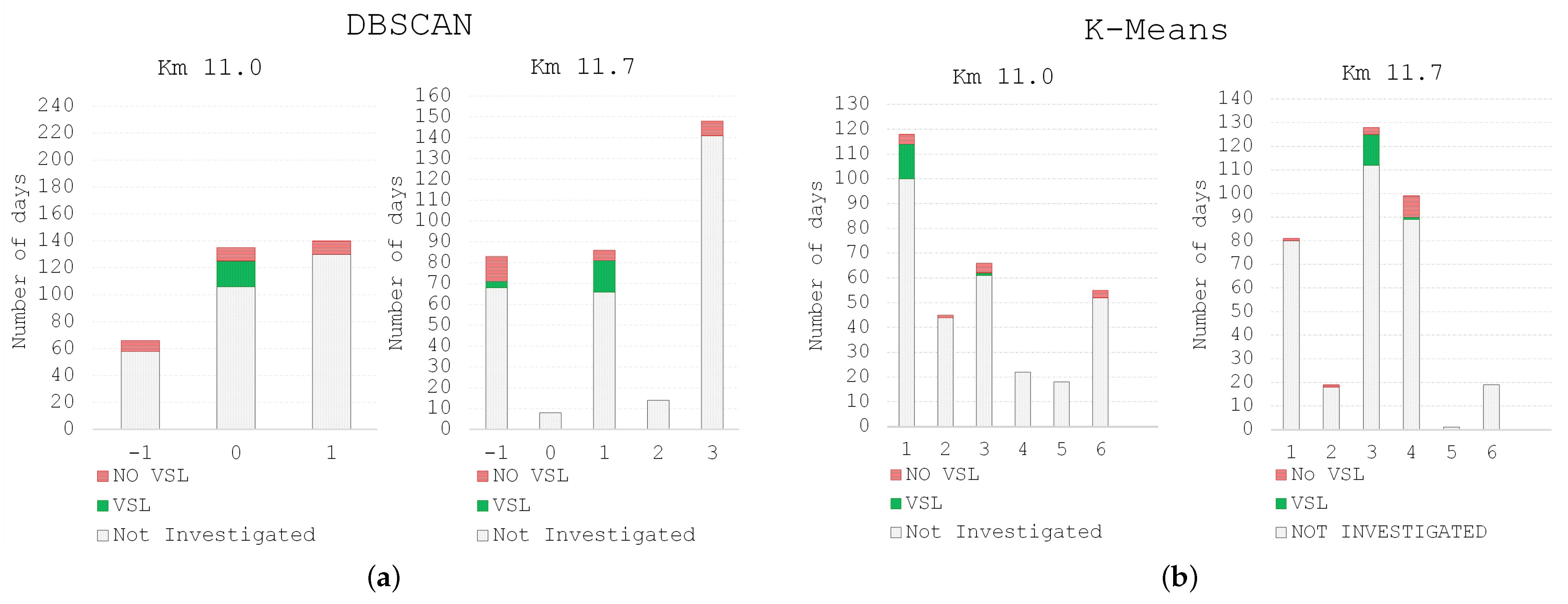
Further analysis considered the distribution of the number of days into different clusters, with reference to the 40 days of recurring congestion observations. The cluster analysis was performed on every day in the whole observation period; however, the comparative analysis of the VSL system is limited to 40 days with observed recurring congestion conditions and similar flows (19 days with VSL active and 21 without VSL). As far as the cluster analysis, the other days were not investigated because of the identification of the other factors, but VSL activation is out of the scope of this study. The distribution of the number of days forming different clusters for the count locations at km 11.0 and at km 11.7, situated in the area where the congestion is normally formed, is reported in Figure 11.

DBSCAN algorithm individuated two clusters for the count location situated at km 11.0 and four clusters for the count location situated at km 11.7; analyzing the results, it becomes evident that the cluster −1 refers to the days classified as outliers. For both count locations, most of the days when the system was active are assigned to a unique cluster, while the days when the system was not operating are distributed to different clusters.

Similar results are provided by the K-Means algorithm, which categorized the data into six clusters, as specified earlier. Also, in this case, almost all the days when the system was operating are attributed to a distinct cluster, namely cluster 1 for km 11.0 and cluster 3 for km 11.7, while the days when the VSL was not active are assigned to different clusters.

These results are in line with the statistical analysis and suggest that the observations of the recurring congestion relative to the days when the VSL system was active were similar in terms of the observed speed, while the days when the VSL system was not operating greater variances were observed among the detected speeds, and therefore the days are distributed to different clusters.

It is also worth noting that labeling most of the days with the activated VSL system in a unique cluster was observed mostly for the congested sections, while upstream and downstream of the congested area, where the traffic conditions remained stable, both clustering algorithms assigned different days to clusters regardless of the state of the VSL system.

As for the observed values of the flows, the results showed that days were distributed to different clusters regardless of the state of the activation of the VSL system, which is also in line with the statistical analysis that did not reveal statistically significant differences for the total distance traveled, affected by the flow values.

4.6. Speed Variance Analysis

Intravehicular variance has been proven to be one of the main factors affecting incident rates [39], and the applications of VSL systems often claim that the reduction of the intravehicular variance is one of the achievements [28,32,35,40]. In this analysis, the variance of the speeds observed on different lanes is assessed for the days of the activated VSL system (VSL) and the days when the system was not operating (No VSL). 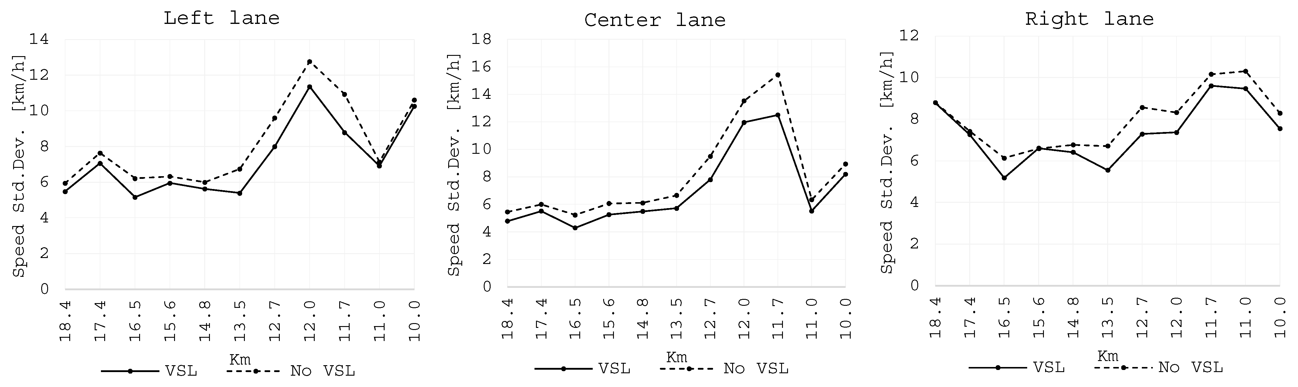Figure 12 reports the profiles of the standard deviation observed for the samples of the days for different traffic lanes.

In general, the variance values assumed higher values when the VSL system was not operating. For the left lane and the center lane, it is evident that the variances increase closer to the point where the recurrent congestion is formed, located between km 11.7 and km 12.0. The highest values of the standard deviation are observed for the center lane, followed by the left lane, and finally, the right lane reports the lowest values.

The average standard deviation was 8 km/h on the days when the VSL system was not operating and reduced to 7 km/h on the days when the system was active. The reduction of the variance is statistically significant for the left lane for the count locations situated at km 11.7 and km 12.0; in the case of the center lane, the statistical significance is obtained for the km 11.0, km 11.7, and km 12.0, while for the right lane, the statistical significance is obtained for the count location situated at km 12.7 downstream from the formed congestion.

Also, the statistical analysis of the variance of the observed flows was conducted. This analysis did not provide any proof of the statistical differences between the days referring to the two cases of the system application.

5. Discussion

The analyses presented in this paper evaluated the impacts of the activation of the VSL system on global motorway performances, considering different aspects of the traffic variables due to the complex spatiotemporal variability of the phenomenon. The assessment, provided by the application of statistical tests together with two specific clustering methods, concerned the speed, the average travel time, and the distance, together with the analysis of the speed variances, which are an important metric of drivers’ behavior affecting safety conditions. The summary of the obtained results is reported in

Table 4. Summary of obtained results.

Measure and Evaluation Result with Respect to No VSL Case
Observed speed distributions: 85th perc. decreased between 10% and 12%
Compliance (suggested VSL VS posted speed): increased between 2% and 8%
Travel time per vehicle during recurrent congestion: decreased by 4%
Variability during recurrent congestion: decreased between 12% and 20% for the speed, not significant results for the flow
Pattern similarities during recurrent congestion: similar speed patterns for the days when VSL was active, not significant results for the flows
Mean distance traveled per vehicle during recurrent congestion: controversial results for different lanes, significant decrease only for the left lane (1%)

.

The Kolmogorov–Smirnov test was applied to assess the differences in the observed speed distributions with and without VSL: on average, around 74% of count locations reported statistically significant results. For the left lane, the 85th percentile of the observed speeds was 119 km/h in the No VSL case and decreased on average by 15 km/h (12%) in the VSL case as the speed limit decreased from 90 km/h to 60 km/h. For the center lane, the 85th percentile passed from 103 km/h in the No VSL case to an average of 93 km/h in the VSL case, with a decrease of 10 km/h (10%). Despite general low values of compliance to the speed limit, ranging between 3% and 53% for different cases, an increase of compliance between 2% and 8% for different lanes was observed when the VSL was active, even in the case of ordinary speed limits, i.e., 90 km/h for the left and center lane and 60 km/h for the right lane, was indicated by VSL.

Similar cases of recurrent congestion were analyzed statistically with and without the VSL activation, using data relative to 40 days with recurrent congestion occurring between km 11.0 and km 14.0 of the Westbound. The average speed (V avg), the mean travel time per vehicle (MTT), and the mean travel distance per vehicle (MTD) distributions were compared by t-test to verify differences in the observations.

The decrease in the mean travel time spent in the case of the application of the VSL system, found to be significant for all lanes, was around 4%. The differences in the mean distance traveled were significant only for the left lane. The corresponding decrease in the VSL case was negligible (0.04 km, corresponding to 1%). The obtained results are comparable to another study of VSL system application [34], where the vehicle miles traveled reported controversial results, and the vehicle hours traveled decreased by 1–6%.

Also, a clustering analysis confirmed the results obtained by the statistical tests. For the locations situated within the recurring congestion area, most days when the VSL system was active were in the same cluster, while the days when the system was not active were distributed to different clusters. These results were obtained independently by the two tested clustering approaches, namely K-Means and DBSCAN. For the locations situated out of the congested area, the state of the VSL system was not relevant, as different days were distributed to different clusters regardless of the state of the VSL system.

The average profiles of the intravehicular variances relative to different count locations were examined, and the results showed significant differences for the count sections situated within the congested area. On the affected count locations on the days when the VSL system was activated, the standard deviation decreased by around 1 km/h (12%) for different lanes with a statistical significance of 95%.

6. Conclusions

The paper presented a field study of an Italian expressway with the implementation of an advisory Variable Speed Limit system, carried out on the data collected by the count locations during almost one year of observations covering cases when the system was active (VSL) and cases when the VSL system was not operating (No VSL).

The analyzed traffic patterns appeared different both by using statistical tests and clustering approach, and improvements in terms of the average speed and the mean travel time were observed in the case of the active VSL system. The distributions of the observed speeds were significantly different in the two cases, and on most data, different speed limits were applied. The analyzed system was advisory without enforcement measures implemented to guarantee compliance rates; thus, the observed differences were moderate, and the compliance level was low.

The obtained results suggest that the VSL system can potentially improve the performance of traffic flow; however, the introduction of enforcement measures aiming to increase compliance levels are to be considered for implementation to empower traffic flow management.

The provided analysis was concerned mostly with the distributions of the observed speed, while the observed flows were analyzed only on a macroscopic level in terms of average values observed by different count locations. However, to make further considerations about the evolution of the traffic propagation process with the application of the VSL system, future research needs to consider aspects of traffic deterioration on the fundamental diagram that relates speed and density.