A Simulated Annealing Approach to the Scheduling of Battery-Electric Bus Charging

Abstract

With an increasing adoption of battery-electric bus (BEB) fleets, developing a reliable charging schedule is vital to a successful migration from their fossil fuel counterparts. In this paper, a simulated annealing (SA) implementation is developed for a charge scheduling framework for a fixed-schedule fleet of BEBs that utilizes a proportional battery dynamics model, accounts for multiple charger types, allows partial charging, and further considers the total energy consumed by the schedule as well as peak power use. Two generation mechanisms are implemented for the SA algorithm, denoted as the “quick” and “heuristic” implementations, respectively. The model validity is demonstrated by utilizing a set of routes sampled from the Utah Transit Authority (UTA) and comparing the results against two other models: the BPAP and the Qin-Modified. The results presented show that both SA techniques offer a means of generating operationally feasible schedules quickly while minimizing the cost of operation and considering battery health.

1. Introduction

With an ever-increasing interest in the electrification of vehicles in the push for green transportation, many organizations and companies have been looking to adopt a fleet of electric vehicles [1]. This transition includes battery-electric buses (BEBs) [2,3]. In particular, agencies such as the Utah Transit Authority (UTA) have directed focus into replacing their fleets with BEBs. Alongside all the benefits that are associated with BEBs come new challenges that must be addressed prior to their integration into mainstream utilization. The energy storage capacity of BEBs is typically significantly less than their combustion counterparts while also having significantly longer refueling periods  [2,4]. This is further complicated due to the care that must be taken in prolonging the lifespan of the battery [5,6,7]. As another complication, BEB refueling is not a fixed cost (i.e., price per gallon multiplied by tank size). Utility companies, in addition to charging for the total energy consumed over a pay period, often charge a demand cost. The demand cost is based on the peak power drawn during the pay period and can significantly impact the overall monetary cost of maintaining the BEBs. To address these limitations, this work introduces a static scheduling framework for a fleet of BEBs that aims to minimize charging costs while considering other constraints pertinent for operation.

A host of strategies have been proposed to solve the BEB charger scheduling problem. Strategies vary in terms of their basic formulation, primarily using variations of the vehicle scheduling problem (VSP) which emphasize the generation of BEB routing schedules, but take little consideration as to how the BEBs are assigned to chargers [8,9,10,11,12,13,14]. In [15,16], the work directly addresses the charger scheduling problem by creating a mixed integer linear program (MILP) that utilizes a network flow approach to generate static charging schedules given a schedule of BEB routes. Similarly, Ref. [17] developed an MILP that generates a static charging schedule by utilizing a rectangle packing approach, referred to as the position allocation problem (PAP). Some works assume that BEBs always charge to full capacity each time they connect to a charger  [8,9,14,18,19]. Other works allow for partial charging using a linear battery charge model  [13,16,20,21,22] or utilize a higher-fidelity, nonlinear battery model  [8,15,23,24,25]. Some works consider only fast chargers during planning [12,14,20,21,22,26,27,28], while others assume that different types of chargers can exist in different locations  [11,13].

When considering the utility rate schedules, two key elements must be considered: the consumption cost and the demand cost. Most approaches consider a consumption cost  [9,10,16,18,23,24,25,26]. This is akin to the combustion engine fuel cost. Fewer works, however, consider the demand cost  [13,16,23,24,25]. The demand cost calculation requires a fine sampling of the power usage at any given time. Approaches that assume a full charge whenever the bus connects typically employ a coarse sampling of charger time periods and may not be well suited to demand cost calculations. Furthermore, the assumption of always using fast chargers is adverse to battery health  [6,7,18].

To accurately calculate the demand cost, an inherent trade-off exists between the low computation of a representative linear model and the high computation of a high-fidelity nonlinear model. A linear, proportional model is used in this work as they have been shown to be accurate below an 80% threshold [2]. This is considered sufficient for this work as charging a battery nearly to capacity is detrimental to the health and can significantly reduce the total charge cycles a battery may undergo  [6,7]. Thus, staying within the linear operating region is desirable for battery health.

The contributions of this work lie in the adaptation and enhancement of [17] to develop a novel formulation by employing a simulated annealing (SA) framework that generates static charging schedules and considers (1) different types of chargers at the same location, (2) minimization of the consumption and demand utility costs, and (3) partial charging through a representative linear charge model. Particularly, this work addresses the gap in the literature by expanding the work of [17] by reimplementing the MILP, utilizing a meta-heuristic approach and examining its performance while further considering demand cost. These contributions are demonstrated via simulation and compared to two other models: an implementation of the PAP for BEBs, denoted as BPAP, and what is known as the Qin-Modified technique.

The remainder of this paper is as follows. Section 2 provides the problem statement associated with this work. Section 3 provides a description of the input parameters and decision variables, then introduces the structure of the formulation. In Section 4, the concept and theory of SA is introduced. In particular, the algorithms and methods utilized for the SA implementation for this work are discussed. Section 5 combines the previous sections to introduce the particular pseudocode for the SA PAP. In Section 6, an example problem is provided to demonstrate the capability of the work provided in this paper. The results are then presented and discussed.

2. Problem Description

Consider a fleet of BEBs scheduled to perform a set of prescribed routes on a given day. An individual BEB from said fleet begins and completes an individual route at the same station from which it also receives its charge. During each route, the BEB’s state of charge (SOC) is depleted by a certain amount. The charge supplied during its visit must be enough to sustain the BEB’s SOC at an appropriate level so that it may complete its next route. Provided there is a set of chargers at the station, the bus may be placed in any single queue to receive its charge. Let the term “arrival” describe the time at which a BEB reaches the station. Furthermore, let the term “visit” denote a BEB having arrived, awaited its predetermined time (whether it has received a charge or not), and departed from the station. Each BEB is allowed to have multiple visits throughout the working day.

Because each bus may visit the station more than once, let the previously considered fleet contain $n_B$ BEBs that collectively visit a station $n_V$ times. At said station, let there exist a pool of $n_Q$ charging queues from which a visiting BEB may be assigned. Upon arrival to the station, a bus is admitted to one of the $n_Q$ queues for charging. Each queue represents a charger that supplies the bus with a charge at a particular rate or allows the bus to sit idle when no charging is required (i.e., a charge rate of zero). The set of possible queue indices is denoted as $Q\in \{1,\dots ,n_Q\}\subset \mathbb{Z}$, where $\mathbb{Z}$ is the set of integers. It is assumed that charger $q\in Q$ has an associated charge rate, denoted as $r_q$. Let the set of arrivals be written as $I=\{1,\dots ,n_V\}\subset \mathbb{Z}$, and let each BEB be prescribed an identification number from the set $B=\{1,\dots ,n_B\}\subset \mathbb{Z}$. As such, each visit can be represented by the tuple: $(i,b,a,e,u,d,q,\eta ,\xi )$, in which the elements within the tuple denote the visit index, $i\in I$, BEB identification number, $b\in B$, arrival time to the station, $a\in \mathbb{R}$, departure time from the station, $e\in \mathbb{R}$, time at which the BEB begins charging, $u\in \mathbb{R}$, time at which the BEB ends charging, $d\in \mathbb{R}$, the charger queue for the BEB to be placed into, $q\in Q$, the SOC upon arrival, $\eta \in \mathbb{R}$, and the index of the next visit for the currently visiting BEB, $\xi \in I\cup ⌀$. The null element, ⌀, is used to specify when a BEB has no future visits. Let the set of visits be denoted as $\mathbb{I}$, where the $i\mathrm{th}$ visit is denoted is ${\mathbb{I}}_i$. Furthermore, let a particular item from the tuple for visit i be written as ${·}_i$. For example, the arrival time for visit i is written as $a_i$.

The amount of time a BEB is allowed to charge during visit i is dictated by the scheduled arrival time and required departure time, $[a_i,e_i]$. Partial charging is allowed; however, the SOC may not exceed the BEB battery capacity, ${\kappa }_b$, and the SOC is desired to stay above some minimum percentage of the battery capacity, ${\nu }_b\in [0,1]$. The battery dynamics in this work are modeled as linear, and remain accurate up to about an SOC of 80% [22]. Note that excessively charging the BEBs is undesirable due to battery health concerns, as at higher SOCs, overshoot becomes a concern and may also cause the battery to undergo deep cycles, which may accelerate battery degradation [6,7].

Each BEB arrival, except for the last arrival for each BEB, has a paired “route” that the BEB must perform after the visit. This route, as one would expect, causes the BEB to discharge by some certain amount. Each bus route is assumed to have a fixed discharge. Let the discharge of the route for visit i be denoted as ${\Delta }_i\in \mathbb{R}$. Note that the last visit for each BEB does not have an associated route, implying that there is no discharge after these particular visits, i.e., ${\Delta }_i=0$ for all i corresponding to a final visit.

3. Optimization Problem

The optimization problem outlined in this work is presented in form of an objective function with constraints. The constraints ensure that candidate solutions are operationally feasible. The variables of optimization are introduced in Section 3.1, followed by a discussion of the constraints in Section 3.3. The objective function is employed to allow relative comparisons between candidate solutions and is introduced in Section 3.2.

3.1. Variable Definitions

This section defines the input and decision variables used in this work. The definitions used in this work are summarized in the Nomenclature section.

3.1.1. Input Parameters

Parameters are used to indicate values that are assumed to be known prior to optimization. They will be presented in two sections: packing and discretization parameters, then battery dynamic parameters. The spatiotemporal parameters are those that ensure no scheduling overlap in either space or time. The discretization parameters describe the parameters that discretize the time horizon, and the battery dynamic parameters are those associated with the SOC of the BEB.

Spatiotemporal and Discretization Parameters

As previously introduced, ${\xi }_i$ represents the next arrival index for bus $b_i$. As an example of its use, suppose the ID of each BEB is recorded in order of arrival as $\{2,1,3,2\}$. Using a starting index of 1, ${\xi }_1=4$, as that is the next visit by bus 2. Each visit is prescribed arrival and departure times, $a_i$ and $e_i$, respectively. An associated cost is employed when a visit is assigned to a charging queue. Let the assignment cost be represented by ${ϵ}_q$. Lastly, the time horizon is to be discretized to assist in computing the peak demand cost; let $t_h$ denote a discrete time step, and let $dt$ denote the discrete time step $dt=t_h-t_{h-1}$.

Battery Dynamic Parameters

It is assumed that each bus begins the working day with an initial SOC percentage of ${\alpha }_b$. Let the set of initial visits by each BEB be denoted as $I_0$, where $I_0\subset I$ and the cardinality of the set is $\left|I_0\right|=n_B$. The initial SOC for bus $b_i$ can be represented as ${\eta }_i={\alpha }_{b_i}{\kappa }_{b_i};\forall i\in I_0$ where ${\kappa }_{b_i}$ is the battery capacity for bus $b_i$. After each arrival, the BEB is assigned to a charging queue. Let $r_q$ represent the power supplied from the charger in queue $q\in Q$. Each visit, except for the final visit of each BEB, is paired with a subsequent route to be executed with a corresponding energy requirement, ${\Delta }_i$. As alluded to earlier, there are no routes after the last visit for each BEB. Thus, similarly to the set of initial visits, let the set of final visits for all BEBs be denoted as $I_f$. The discharge for the final visit of each BEB is then defined as ${\Delta }_i=0;\forall i\in I_f$.

3.1.2. Decision Variables

Decision variables are those chosen by the optimizer. There are three direct decision variables for each visit: the initial and final charging times, $u_i$ and $d_i$, respectfully, and the selected charging queue, $q_i\in Q$.

The remaining variables are slack variables, which are introduced to track the vehicle charge and queuing position based on the parameters and direct decision variables. Recall that the initial SOC for a visit is written as ${\eta }_i$, where $i\in I\setminus I_0$. Further, recall that the set of initial visits, $I_0$, have an assumed known SOC. The charge for bus i’s next visit is equal to the initial charge for visit i plus the charge added to it by charger $q_i$ over duration $s_i=d_i-u_i$ minus the discharge accumulated after visit i, ${\eta }_{{\xi }_i}={\eta }_i+r_{q_i}{s}_i-{\Delta }_i$.

The variables ${\sigma }_{ij}$ and ${\psi }_{ij}$ are used to indicate whether a visit pair $(i,j)$ overlap the same space, as shown in Figure 1. These spatiotemporal variables uphold the following relationships: for every visit, ${\sigma }_{ij}=1\Rightarrow$ that the start charge time of visit j is greater than the end charge time of visit i. Similarly, ${\psi }_{ij}=1\Rightarrow$ the queue for visit j is of a greater index than visit i. A value of zero for either of these variables conveys no information. The variable $\mathbb{C}$ is the set that describes the availability for all chargers. That is, $\mathbb{C}$ is a set of $n_Q$ sets that contain available charger times for each queue $q\in Q$. Let a set of available charge times for queue q be defined as ${\mathbb{C}}_q$.

3.2. Objective Function

This work aims to minimize the total “cost” of utilizing a given charge schedule. Let $J\left(\mathbb{I}\right)$ represent the objective function. The objective function for this problem has four main considerations: an assignment cost, a penalty method for visits with insufficient SOCs, consumption cost, and a demand cost, each of which will be discussed in turn throughout the subsequent sections.

3.2.1. Assignment Cost

The assignment cost represents the cost of assigning a bus to a queue. Particularly, the cost consists of summing a prescribed weight for the selected charger, ${ϵ}_{q_i}$, multiplied by the charge rate, $r_q$. Formally, the cost is written as follows:

$$\sum _{i=1}^{n_V}{ϵ}_{q_i}{r}_{q_i}.$$

(1)

This is effectively the cost of selecting queue $q_i$. While any set of weights may be selected, Section 6 uses a particular choice for the assignment cost to encourage the use of slow chargers over fast for the sake of battery health. The charger queue indices are ordered such that the first $n_B$ queues correspond to idle queues. This allows all BEBs to simultaneously sit idle if needed. All $n_B$ idle queues have assignment costs of zero to denote that there is no cost when not charging. The next group of chargers is assumed to be the slow chargers subsequently followed by the fast. Letting $P\in \mathbb{R}$, then the set of slow and fast charging queues are of the form $[P,2P,\dots ,n_{Q}P]$. Concatenating these vectors yields $ϵ=[0,0,\dots ,P,2P,3P,\dots ]$, where $ϵ$ describes the vector of assignment costs, and the first $n_B$ values are zero.

3.2.2. Penalty Method

A penalty method is to be implemented to provide a soft constraint on the lower bound of the charge. Due to the uncertainty of the initial SOC for each visit, a soft constraint is desired to increase the solution space while penalizing nonoperationally feasible solutions. If a hard constraint were to be implemented, the constraint would restrict the set of allowable schedules to only operationally feasible schedules. Let the piecewise function that enables/disables the penalty method be of the form

$$\varphi \left(x\right)=\left\{\begin{array}{cc}0\hfill & x\ge 0\hfill \\ x^2\hfill & x<0.\hfill \end{array}\right.$$

(2)

Letting x be defined by the difference of the initial SOC for visit i, ${\eta }_i$, and the minimum charge threshold, ${\nu }_{b_i}{\kappa }_{b_i}$, applies a penalty proportional to the difference of the SOC and the threshold squared. That is, $x={\eta }_i-{\nu }_{b_i}{\kappa }_{b_i}$. A scalar, $z_p$, is added which can be utilized either as a monetary conversion or a simple gain. This method is employed as a means of encouraging that the schedule has enough charge for each BEB to complete its next route. Therefore, the penalty method is written as

$$\sum _{i=1}^{n_V}{z}_p{\varphi }_i({\eta }_i-{\nu }_{b_i}{\kappa }_{b_i}).$$

(3)

3.2.3. Consumption Cost

In most cases, utility companies have a portion of the cost related to the total electricity consumed over a billing period, referred to herein as the consumption cost. The consumption cost is the summation of all the energy being used over all the active periods for each charger in the time horizon. A scaling $z_c$ is applied as a weight on the summation (this could correspond to a monetary cost imposed by the utility). This is represented by the summation

$$z_c\sum _{i=1}^{n_V}{r}_{q_i}{s}_i.$$

(4)

3.2.4. Demand Cost

Utility companies often charge a “demand cost” in an effort to reduce peak power use. A particular example of peak demand is the fifteen-minute average energy usage employed by Rocky Mountain Power Schedule 8 [29].

A method of calculating the demand charge is to calculate the average power consumption over a given period of time. Let the average power used over an arbitrary interval, $T_p$, be represented by

$$p_{T_p}\left(t\right)={\displaystyle \frac{1}{T_p}}{\int }_{t-T_p}^{t}p\left(\tau \right)d\tau .$$

(5)

The largest average power usage over $T_p$ is used as the demand cost for the billing period. Therefore, let the cost of the peak power consumption be dictated by the maximum average power: $p_{max}\left(t\right)=\underset{\tau \in [0,t]}{max}{p}_{T_p}\left(\tau \right)$. Furthermore, a fixed minimum average power is introduced that is intended to act as a base threshold before the cost begins to increase. Let this fixed threshold be defined as $p_{fix}$, and the demand cost is calculated using $p_d\left(t\right)=max(p_{fix},p_{max}\left(t\right))$. For the sake of implementation, the integral in Equation (5) is discretized. Let $dt$ denote the discretization time step and let $p_h$ denote the power for the $h^{\mathrm{th}}$ step. Equation (5) is approximated as $p_{T_p,h}={\displaystyle \frac{1}{T_p}}{\sum }_{k=h-{\displaystyle \frac{T_p}{dt}}+1}^h{p}_{k}dt$. The discrete demand cost is expressed as $p_d=max(p_{fix},p_{max})$. Similarly to the consumption cost, a scaling $z_d$ is applied. Again, this may be a monetary conversion or simply just a gain. The objective function written in its entirety is

$$J\left(\mathbb{I}\right)=z_d{p}_d+\sum _{i=1}^{n_V}\left[{ϵ}_{q_i}{r}_{q_i}+z_p{\varphi }_i({\eta }_i-{\nu }_{b_i}{\kappa }_{b_i})+z_c{r}_{q_i}{s}_i\right].$$

(6)

3.3. Constraints

While the objectives are used to compare solutions, constraints are introduced to ensure that the solutions are operationally valid. Operational validity requires that allocated BEBs do not overlap spatially or temporally. Furthermore, the SOC of a bus at a particular visit is related to the charge from its previous visit by the amount of charging and discharging that has occurred. Finally, buses must leave the charger before their scheduled departure time. These constraints are represented as follows:

$$u_j-d_i-({\sigma }_{ij}-1)T\ge 0$$

(7a)

$$q_j-q_i-1-({\psi }_{ij}-1)Q\ge 0$$

(7b)

$${\sigma }_{ij}+{\sigma }_{ji}\le 1$$

(7c)

$${\psi }_{ij}+{\psi }_{ji}\le 1$$

(7d)

$${\sigma }_{ij}+{\sigma }_{ji}+{\psi }_{ij}+{\psi }_{ji}\ge 1$$

(7e)

$$s_i=d_i-u_i$$

(7f)

$${\eta }_{{\xi }_i}={\eta }_i+r_{q_i}{s}_i-{\Delta }_i$$

(7g)

$${\kappa }_{b_i}\ge {\eta }_i+r_{q_i}{s}_i$$

(7h)

$$a_i\le u_i\le d_i\le e_i\le \mathcal{T}$$

(7i)

Equations (7a)–(7e) are denoted as “queuing constraints”. They prevent overlap both spatially and temporally, as shown in Figure 2. The x- and y-axis of Figure 2 represent time and space, respectively. Along the y-axis, the dashed lines represent discrete queuing locations. The shaded rectangles represent schedules BEBs to be charged. The vertical position of each shaded rectangle represents the BEB’s assigned queue. The width of the shaded rectangles represent the time to service the BEB. The vertical dashed lines are associated with vessel D and represent the arrival time, initial charge time, charge completion time, and departure time. Note that the arrival time may be before the initial charge time and the completion time may before the departure time. In other words, the set of constraints Equations (7a)–(7e) aim to ensure that these shaded rectangles never overlap.

Constraint Equation (7a) states that the starting charge time for BEB $u_j$ must begin after the previous BEB departs, $d_i$. A value of ${\sigma }_{ij}=1\Rightarrow$ bus i has detached from the charger before bus j has begun charging. If ${\sigma }_{ij}=0$, then the constraint is of the form $\mathcal{T}+d_i>u_j$, rendering the constraint “inactive”. Similarly, for Equation (7b), ${\psi }_{ij}$ determines the spatial positioning of BEB i and j relative to one another. A value of ${\psi }_{ij}=1\Rightarrow$ BEB i is in a queue index that is less than BEB j. If ${\psi }_{ij}=0$, then the constraint is deactivated. Constraints Equations (7c)–(7e) enforce spatial and temporal ordering between each queue/vehicle pair. Equations (7c) and (7d) ensure that BEB i is not placed before and after j spatially or temporally as that is not possible. Equation (7e) enforces that at least one of the spatial or temporal relationships between each visit is active. This ensures that there are no scheduling conflicts (i.e., either charging sessions are ordered temporally or are in different queues).

Equation (7f) describes the service time of the bus. Equation (7g) calculates the initial charge for the next visit for bus $b_i$. Equation (7h) ensures that the bus is not being overcharged. Equation (7i) ensures the continuity of the times (i.e., the arrival time is less than the initial charge, which is less than the detach time, which is less than the time the bus exits the station, and all must be less than the time horizon).

4. Simulated Annealing

SA is a well-studied local search metaheuristic used to solve various optimization problems [30,31]. The algorithm is often applied to problems that contain many local solutions as it employs a stochastic approach that explores the solution space for an approximate global optimum. This model is named after its analogized process, where a crystalline solid is heated then allowed to cool at a slow rate until it achieves its most regular possible crystal lattice configuration (i.e., lowest energy state) [31,32]. SA establishes a connection between the thermodynamic process and the search for global optimum in optimization problems. Within the SA process there are three key components: cooling equation, acceptance criteria, and generation mechanisms [31,33].

The cooling equation describes the speed at which the figurative temperature is decreased in a controlled manner over time. Throughout the SA process, many “candidate” solutions are generated and compared to an “active” solution. The method by which the solutions are accepted is determined by the acceptance criteria. The acceptance criteria is a function of the system temperature that makes the decision whether the system will accept an inferior solution in favor of exploring the solution space. The means by which candidate solutions are generated are via the generation mechanisms. These generators modify the solution by some singular discrete change [30]. Each of these components are elaborated in the subsequent sections.

4.1. Cooling Equation

The cooling equation models the rate at which the temperature decreases over time in the SA process. Initially, when the temperature is high, SA encourages exploration. As the process begins to “cool down” (in accordance to the cooling schedule), it begins to encourage local exploitation of the solution (rather than exploration) [32,34]. There are three common basic types of cooling equations: linear, geometric, and exponential. The geometric cooling schedule is most widely used in practice [33]. As such, it will also be employed by this work. It is defined by the difference equation

$$t_m=\beta t_{m-1}.$$

(8)

In Equation (8), $\beta$ controls the cooling rate. Typical values of $\beta$ are within the range $[0.8,0.99]$ [32]. The variable $t_m$ represents the temperature at the $m\mathrm{th}$ step of the temperature function. The total number of steps, M, is dictated by the initial temperature and $\beta$.

4.2. Acceptance Criteria

In SA, the algorithm stores a solution that is continuously compared to newly generated solutions. Let the stored solution be referred to as the “active solution”. During each iteration, a new “candidate” solution is generated and compared to the active solution to determine if the candidate solution should replace the active solution. The method of determining whether the active solution should be replaced is defined by an acceptance criteria. In an effort to encourage exploration, inferior candidate solutions have a probability of being accepted. The probability of accepting an inferior candidate solution is determined by the objective functions of the active and candidate solutions, $J\left(\mathbb{I}\right)$ and $J\left(\overline{\mathbb{I}}\right)$, respectively, and the current temperature, $t_m$. Let $\Delta E\equiv J\left(\mathbb{I}\right)-J\left(\overline{\mathbb{I}}\right)$ and let $f(·)$ be the function that describes the probability of accepting a candidate solution $\overline{\mathbb{I}}$. The probability of accepting a candidate solution is, thus, of the form [33]

$$f(\mathbb{I},\overline{\mathbb{I}},t_m)=\left\{\begin{array}{cc}1\hfill & \Delta E>0\hfill \\ e^{-{\displaystyle \frac{\Delta E}{t_m}}}\hfill & \mathrm{otherwise}\hfill \end{array}\right..$$

(9)

4.3. Neighbor Generators and Wrappers

Generation mechanisms are used to create a neighboring candidate solution [30]. That is, the generating function creates a solution that can be reached in a single iteration from the active solution. In response to the problem statement made in Section 2, five primitive generation mechanism are used: new visit, slide visit, new charger, wait, and new window. The purpose of each of these generators is to assign new visits to a charger, adjust a bus visits initial and final charge time within the same time frame/queue, move a BEB from one charger to another with the same charge schedule, and move a bus to its idle queue. Each generator will be discussed in more detail in Section 4.3.2.

These primitive generation mechanisms will, in turn, be utilized by two wrapper functions. The charge schedule generator is to used create an initial candidate solution for SA and the perturb schedule generator is used to take a candidate solution and alter it slightly in an attempt to step toward a global or local minimum. The wrapper functions will be discussed in Section 4.3.3. However, prior to discussing the primitives and wrapper generating functions, their respective inputs and outputs must be defined.

4.3.1. Generator Input/Output

Each generator primitive accepts a tuple $\mathbb{S}\equiv (i,\mathbb{I},\mathbb{C})$, where i is the visit index being manipulated, $\mathbb{I}$ is the set of visits, and $\mathbb{C}$ is the set that describes the availability for all chargers $q\in Q$. The output of the generating functions is the same as the input, but with changes applied to it by a generator. Let a modified variable be denoted with a bar, $\overline{·}$. Thus, the modified input tuple is written as $\overline{\mathbb{S}}$.

4.3.2. Generators

The mechanism by which candidate solutions are generated are now introduced. For the sake of ease in referring to the various variables associated with a visit, dot notation is used. For example, suppose the arrival time is desired to be extracted from visit i. Given $\mathbb{I}$, the notation that describes extracting the initial charge time for visit i is written as $u_i\equiv {\mathbb{I}}_{i.u}$.

New Visit

The new visit generator defined in Algorithm 1 describes the process of moving a BEB, $b\in B$, from a waiting queue, $q\in B$, to a charging queue, $q_i\in \{n_B+1,\dots ,n_Q\}$, within its arrival/departure time $[a_i,e_i]$. Let ${\mathcal{U}}_{\{·\}}$ indicate that an element is selected randomly with a uniform distribution from the set $\{·\}$. For example, ${\mathcal{U}}_{[a_i,e_i]}$ indicates that a value will be selected between a and e with a uniform distribution. Algorithm 1 begins by extracting variables. Lines 8 and 9 randomly select a charging queue and available time frame with a uniform distribution, respectively. Line 10 attempts to assign the visit to the previously selected time slice; if it succeeds, the updated visit is returned. Otherwise, the null value is returned.

The function FindFreeTime is the algorithm that determines whether a visit’s time at the station $[a_i,e_i]$ can be placed in the time availability of charger q. Let the available time for charger q for visit i be denoted as $C\equiv {\mathbb{C}}_{i.q}$. Furthermore, let the lower and upper bound of $\mathbb{C}$ be denoted as $C_L$ and $C_U$, respectively. The algorithm checks whether the BEB time at the station, $[a_i,e_i]$, fits within the charger availability $[C_L,C_U]$. If it does, a random charging time frame is returned such that $a_i\le u_i\le d_i\le e_i$. Otherwise, the null value is returned.

Algorithm 1: New visit algorithm.

Slide Visit

This primitive generator is used for visits that have already been scheduled. Because of the constraint Equation (7i), there may be some slack to manipulate $[u_i,d_i]$ within the window $[a_i,e_i]$. That is, two new values, $u_i$ and $d_i$, are randomly selected with a uniform distribution that satisfy the constraint $a_i\le u_i\le d_i\le e_i$. Algorithm 2 begins by extracting variables. Line 5 purges the visit from the charger availability schedule. The Purge function simply removes an assigned charge time from the set $\mathbb{C}$. Without altering selected queue, the charge time is randomly reassigned with a uniform distribution. Upon success, the updated tuple is returned, otherwise the null value is returned.

Algorithm 2: Slide visit algorithm.

New Charger

The new charger generator moves a visit ${\mathbb{I}}_i$ to a new charging queue while maintaining the same charge time, $[u_i,d_i]$. Algorithm 3 begins by extracting variables, and then purges the visit from the charger availability set. A queue is selected at random with a uniform distribution, then the new selection is checked for whether the charge time $[u_i,d_i]$ may be assigned to the new queue.

Algorithm 3: New charger algorithm.

Wait

The wait generator simply removes a bus from a charger queue and places it in its idle queue, $q_i\in B$. Algorithm 4 begins by purging the visit from the charger availability set; the visit is then assigned to its idle queue for the duration of its time at the station.

Algorithm 4: Wait algorithm.

New Window

New window, as shown in Algorithm 5, is a combination of Algorithm 1 (new visit) and Algorithm 4 (wait). By this, it is meant that visit i is placed in its wait queue then added back in as if it were a new visit. This implies that the BEB may be assigned to a different queue with a new charging time frame. Upon success, the algorithm returns the updated tuple; otherwise, it returns the null value.

Algorithm 5: New window algorithm.

4.3.3. Generator Wrappers

The generator wrappers provide the highest level of abstraction from which the SA algorithm directly interacts. These wrapper functions utilize the primitive generators previously described to either create a new charge schedule to initialize the SA algorithm, or to modify an existing schedule.

Charge Schedule Generation

The objective of Algorithm 6 is to introduce a method that provides the SA algorithm with an initial charging schedule. The schedule generation is chosen to initialize the algorithm in a greedy manner by looping through each visit and executing Algorithm 1 to place visit i at a random queue with a random charge time.

Algorithm 6: Charge schedule generation algorithm.

Perturb Schedule

Algorithm 7 describes the method by which the SA algorithm decides how to perturb a given charge schedule. The method that will be employed to generate neighboring solutions is as follows: Pick a visit, pick a primitive generator, and execute said primitive generator once. Let ${\mathcal{W}}_{[·]}^y$ denote a random selection with a distribution specified by a weight vector $y\in \mathbb{R}$. Lines 2–12 of Algorithm 7 generate a vector of weights for the visit index selection. The weights have a default value of one. Each visit is then indexed in reverse order. If the SOC of the visit is less than ${\nu }_b{\kappa }_b$, then the weight for the visit is calculated as shown on Line 10. The route for BEB b is then set as a “priority” on Line 9 to propagate the previously calculated weight to earlier visits of BEB b, as shown in Line 5. This is performed in an attempt to encourage the SA algorithm to “fix” the current or previous visits so that the SOC stays above the minimum threshold. The algorithm then selects a visit index with weighted distribution $y^v$ and selects a primitive with a weighted distribution, $y^p$. Letting $n_G$ denote the number of primitive generating functions, line 15 selects a primitive generating function with a weighted distribution, ${\mathcal{W}}_{[1,n_G]}^{y^v}$. The primitive is then executed, and the results are returned.

Algorithm 7: Perturb schedule algorithm.

4.4. Alternative Heuristic Implementation

As suggested by the works in [35,36], applying heuristics to the generating functions can manipulate the searched neighborhoods in a way that may assist the SA algorithm with convergence. As a test to assist in minimizing charger utilization, a simple heuristic is applied to Algorithms 1 and 3 in the method such that they select new charging queues. Rather than selecting a queue at random from $q\in Q$, the algorithm randomly selects whether to place a BEB in a slow or fast charging queue with a weighted distribution favoring slow chargers. Once the charger type has been selected, the algorithm will then begin incrementally attempting to place the BEB in a queue of that type beginning from the smallest index of that charger type. For example, if a BEB has been selected to be placed in a queue with a slow charger, the algorithm begins by attempting to place the BEB in the charger queue $q=n_B+1$. If it is unable to be placed in that queue, it then attempts to be placed in the next queue $q=n_B+2$. This is performed incrementally until all the queues have been exhausted. The objective of this alternative approach is to explore whether the added up-front computation cost by including the heuristic will positively influence the output of the results and to what degree.

5. Optimization Algorithm

This section combines the generation algorithms and the optimization problem into a single algorithm (Algorithm 8). Generally, SA assumes that the generated candidate solutions are within the solution space of the problem, $\mathbb{S}\in S$, where S is the solution space. In other words, the initialization and perturbations of a schedule must be verified to ensure that the generated schedule is in the solution space. Therefore, the objective function and constraints introduced in Section 3.2 and Section 3.3, respectively, must be employed to verify that the outputs of Algorithms 6 and 7 are in the feasible space, S.

As previously stated, the generating functions directly influence the values of the assigned charge queue, charge initialization time, and charge completion time: $q_i$, $u_i$, and $d_i$, respectively. Having generated those values, the rest of the decision variables may be derived. Beginning with the packing constraints, Equations (7a) and (7b) are employed to enable and disable ${\sigma }_{ij}$ and ${\psi }_{ij}$ and Equations (7c) and (7e) ensure the validity of the values. Equation (7f) can be directly calculated and Equation (7i) is fully defined.

Changing the focus over to the dynamic constraints, similarly to what was seen with the packing constraints, the battery dynamic constraints are also fully defined. Equation (7g) is sequentially calculated after a given schedule has been created. Equation (7h) is evaluated to ensure that the BEB is not overcharged. The penalty method implemented in Section 3.2 is set in place to allow the SOC to go below the specified threshold, ${\nu }_{b_i}{\kappa }_{b_i}$, but to punish the solution for doing so. Thus, over time, the candidate solutions will be encouraged toward a solution that does not activate the penalty method (i.e., the solution is operationally feasible).

The implementation of the SA PAP, outlined in Algorithm 8, will now be discussed. The algorithm begins by creating a temperature schedule and creating an initial solution. The algorithm then iterates through the temperature schedule (outer loop). For each iteration of the outer loop, an inner loop is executed $n_K$ times. During this inner loop, the solution is modified by a primitive generating function to create a candidate solution. The candidate solution is then compared with the active solution, and updated according to the acceptance criteria. These actions are performed until the cooling equation is exhausted.

Algorithm 8: Simulated annealing approach to the position allocation problem.

6. Example

An example is now provided to demonstrate the utility of the developed SA charge scheduling technique. In Section 6.1, a description of the example scenario is presented, followed by a brief introduction of the BEB implementation of the PAP (BPAP) and an alternative threshold based strategy called the Qin-Modified technique. Section 6.2 presents the results for each of the planning strategies. The results are then analyzed and discussed.

6.1. BEB Scenario

The test scenario was run over a time horizon of $T=24$ h, with a total of $n_V=338$ visits to the station shared between $n_B=35$ buses. Each BEB is assumed to have a battery capacity of ${\kappa }_b=$ 388 kWh that is required to stay above an SOC of ${\nu }_b=$ 25% (97 kWh). Each bus is assumed to begin the working day with $\alpha =$ 90% charge (349.2 kWh). A total of 30 chargers are utilized, where 15 of the chargers are slow charging (30 kW) and 15 are fast charging (911 kW). The gains of $z_p=$ 5000, $z_c=1$, and $z_d=$ 10,000 are used. As previously introduced, to encourage slow charging for battery health, the values of $ϵ$ in the objective function are $\forall q\in \{1,2,\dots ,n_B\};{ϵ}_q=0$ and $\forall q\in \{n_B+1,n_B+2,\dots ,n_Q\};{ϵ}_q=10q$. The SA algorithm utilizes the geometric cooling schedule with an initial temperature of $T_0=$ 9000 with $\beta =0.997$, resulting in a total of $n_M=$ 3832 steps. Rocky Mountain Power utilizes fifteen-minute intervals to calculate the demand cost [29]. To match the method by which Rocky Mountain Power determines its demand cost, this work employed an interval of $T_p=$ 900 s in its demand cost calculation. A weight vector of $[0.3333,0.3333,0.1667,0.1667]$ is used to influence the distribution of selecting the new charger, new window, wait, and slide visit primitives, respectively. The algorithm also assumes a total of $n_K=500$ iterations for the local search at a constant temperature with a time horizon discretization of $n_H=$ 1140 steps. In total, that results in 1,916,000 configurations being searched in a total runtime of 1532.8 s.

Section 4.4 introduced the idea of an alternative heuristic implementation for the SA algorithm. To distinguish the heuristic implementation from the method derived in Section 4.3, let this implementation be referred to as “heuristic” implementation and the previous as the “quick” implementation due to the fact that it is designed to execute more quickly. Using the same weights for randomly selecting the primitive generators, the heuristic approach further implemented a weighted distribution vector of $[0.75,0.25]$ to decide whether to select a slow or fast charger, respectively. The heuristic approach had a total runtime of 1916 s. The heuristic generators were expected to be slightly slower due to its iterative approach.

The Qin-Modified is a threshold-based strategy that is also employed as a means of comparison with the results of the SA BPAP. The Qin-Modified algorithm is a based on the threshold strategy of [23]. The algorithm was modified slightly to accommodate the case of multiple charger types without a heuristic search for the best charger type. The heuristic is based on a set of rules that revolve around the initial charge of the bus at visit i. There are three different thresholds: low (60%), medium (70%), and high (90%). Buses below the low threshold are prioritized to fast chargers, then they are allowed to utilize slow chargers if no fast chargers are available. Buses between the low and medium threshold prioritize slow chargers first and utilize fast chargers only if no slow chargers are available. Buses above the medium threshold and below high will only be assigned to slow chargers. Buses above the high threshold will not be charged. Once a bus has been assigned to a charger, it remains on the charger for the duration of the time it is at the station, or it reaches 90% charge, whichever comes first.

Another method utilized to compare with SA PAP is the BEB implementation of the PAP [17]. The BPAP implementation is utilized in this work as a benchmark for the other schedules as it is implemented utilizing a commercial solver. The inputs to the system are the same as those discussed above. It is of note that the BPAP does not implement the demand cost in its objective function. In an attempt to compare the solution of the BPAP with the SA output more directly, a similar solve time of 1900 s is utilized. The BPAP was executed using the Gurobi MILP solver [37]. The previously described simulations were run on a machine equipped with an AMD Ryzen 9 5900X 12–Processor (24 core) at 4.95 GHz.

6.2. Results

The schedules generated by each of the methods are presented in Figure 3. For the sake of conciseness of the schedule plots, the waiting queues are excluded. Therefore, rows 0–14 represent slow charging queues and rows 15–29 represent fast charging queues. The hollow circles with an “X” represent the initial charge times, and the horizontal line with the vertical tick signifies the region of time the charger is active. The Qin-Modified schedule utilized two fast chargers and fourteen slow chargers, as can be seen in Figure 3a. The BPAP framework generated a schedule that utilizes three fast charges and four slow chargers, as shown in Figure 3b. The heuristic SA strategy created a schedule with nine slow charger queues and one fast charging queue, as shown in Figure 3c. The quick strategy for the SA algorithm created a schedule utilizing seven slow chargers and two fast chargers, as is demonstrated in Figure 3d. That is to say, while each schedule emphasized the utilization of slow chargers, the Qin-Modified required fast charging most frequently followed by the BPAP, quick SA, and then heuristic SA. At the expense of incorporating more slow chargers than the BPAP, the SA techniques chose to utilize fast chargers less frequently in their respective schedules, showing an emphasis on battery health.

Table 1. Table of mean, min, and max SOC (kWh) for each charging schedule.

	BPAP	Qin-Modifid	Heuristic	Quick
Mean	181.327	248.864	182.004	188.327
Min	97.000	0.000	91.265	94.760
Max	382.930	349.200	387.829	388.000

tabulates the mean, minimum, and maximum SOC upon arrival for each visit. The BPAP requires each BEB to stay above an SOC of 25%, while the quick and heuristic SA approaches heavily penalize a schedule for allowing a BEB to go below the 25% SOC threshold. The BPAP was able to successfully keep the SOC above the threshold while both SA approaches were a few kWh below the threshold. The SOC of the quick SA approach dropped to a minimum of 94.760 kWh and the heuristic had a minimum SOC of 91.265 kWh, as shown in Table 1. Due to the threshold constraint being soft, the SA objective function may find it better to allow a small deficit in the threshold penalty function in favor of another action. As a remedy to ensure that the SA schedules stay above the threshold, a safety factor could be introduced to artificially increase the threshold, $S_f{\nu }_{b_i}{\kappa }_{b_i}$, where $S_f>1;S_f\in \mathbb{R}$.

The Qin-Modified schedule allowed the SOC for one of the BEBs to reach 0%, as shown in Table 1. The Qin-Modified strategy, being a purely reactive model, does not have the foresight to determine whether a set of routes has a particularly taxing route later in the time horizon. As such, and in the case of the example scenario, the BEB that reached a charge of 0% began with a sequence of short routes, much like the other BEBs. However, rather than continuing this trend, these sets of routes had one or two longer routes, which the Qin-Modified algorithm was unable to account for. Interestingly, despite having a bus drop to zero charge, the Qin-Modified strategy had the highest mean SOC, followed by the quick SA, heuristic SA, and then the BPAP.

Figure 4 depicts the power utilized over the time horizon for each model. Referencing Figure 4a, the Qin maintained long periods of steady slow and fast charger use. This is again a symptom of the Qin-Modified strategy placing BEBs on chargers based solely on the SOC upon arrival. The BPAP and SA techniques, having demand peaks in the first half of the time horizon, were able to effectively maintain lower demand profiles during slower moments throughout the day (the SA techniques more so than the BPAP). Figure 4 is also of interest as it shows the peak power demand over the time horizon. The peaks for each schedule are shown in

Table 2. Table of mean and max power demand for each charging schedule.

	BPAP	Qin-Modified	Heuristic	Quick
Mean	176.550	394.130	180.858	186.858
Max	1910.000	2000.000	1150.950	1120.950

. Both the quick and heuristic SA techniques were able to maintain peak power use below 1130 kW, whereas the BPAP and Qin had peaks above 1900 kW, demonstrating significant demand cost reduction.

The total energy consumed by each schedule is shown in Figure 5. The ordering of most energy consumed to least is as follows: Qin-Modified, quick SA, heuristic SA, and the BPAP. The respective energy consumption for each technique is 9459.120 kWh, 4428.670 kWh, 4295.660 kWh, and 4237.200 kWh, with the heuristic SA consuming about 58.5 kWh more than the BPAP. While the quick and heuristic SA techniques were slightly above the BPAP in energy consumption, it is expected that the BPAP would have the lowest consumed energy as it only considers consumption cost. Despite considering peak demand, the SA methods had nearly the same consumption as the BPAP. Referencing Table 1 and Table 2 for the mean SOC and mean demand, respectively, the descending order of consumed energy is correlated to the descending order of the mean SOC and the descending order of the mean power demand. This makes sense as a higher mean SOC implies the chargers being active more often, similarly for the mean demand.

The charger utilization over the time horizon for each method is shown in Figure 6. Figure 6a shows that the Qin and BPAP employed between one and two fast chargers during the first eleven hours of the working day. The Qin heavily utilizes two fast chargers between hours five and eight to charge all the BEBs above the low threshold. Once the BEBs rose above the low threshold, both the Qin and BPAP utilized the fast chargers more sparingly throughout the working day. However, the difference between the BPAP and the Qin use of the fast chargers is that the BPAP is able to utilize the fast chargers only when required, such as when a long route is on the horizon and the BEB requires a higher initial SOC for visit i (as seen with the Qin SOC reaching 0%). A similar result for both the quick and heuristic SA technique can be seen in Figure 6b; however, both SA methods only require one fast charger, albeit more frequently than the BPAP. After the twelfth hour, neither quick nor heuristic SA methods require the use of fast chargers. This observation is predominantly due to the addition of the demand cost and the fact that it is applied throughout the entire working day. This becomes more clear when viewed in reference to Figure 6c,d. Comparing the slow charger use of the BPAP and Qin versus the quick and heuristic SA methods demonstrates that the charging completed by the fast chargers for the BPAP and Qin was heavily subsidized by slow chargers in the quick and heuristic SA techniques. The SA techniques, however, were still able to detect future demands and offset BEBs to the fast charger only when required. This effectively allowed the consumption costs to be reduced so that the SA techniques remained competitive with the BPAP (Figure 5), but the included demand cost allowed both SA methods to perform better than the BPAP with regard to peak demand (Figure 4).

As a final comparison, the scores for the Qin-Modified, quick SA, BPAP, and heuristic SA are shown in

Table 3. Table of objective function scores for each of the schedules.

Schedule	Score
BPAP	18,500,000
Qin-Modified	34,578,526
Heuristic	11,673,937
Quick	11,234,577

. The Qin-Modified strategy naturally has the highest score as it performed the worst in each metric of the objective function. Although the BPAP was able to maintain the SOC of each BEB above the minimum charge threshold, due to large peaks in the power demand in the BPAP schedule, both SA techniques were able to achieve lower scores. In other words, although the SA techniques allowed small breaches in the minimum SOC, the objective function found the quick and heuristic SA schedule configurations to be more desirable than that of the BPAP. The quick SA was able to successfully obtain the lowest score due to its substantial reduction in the demand cost and its smaller breach of the minimum SOC threshold.

7. Conclusions

This work developed an SA implementation of the BEB charge scheduling problem derived from the works of the position allocation problem [17]. The model was designed to encourage the use of slow chargers for battery health, minimize the peak energy consumption, and minimize the total energy consumed. The problem description was provided along with the assumptions made about the structure of the BEB route schedule. The optimization problem was then introduced by describing the components of the objective function and outlining the constraints utilized to ensure that candidate solutions are in the solution space.

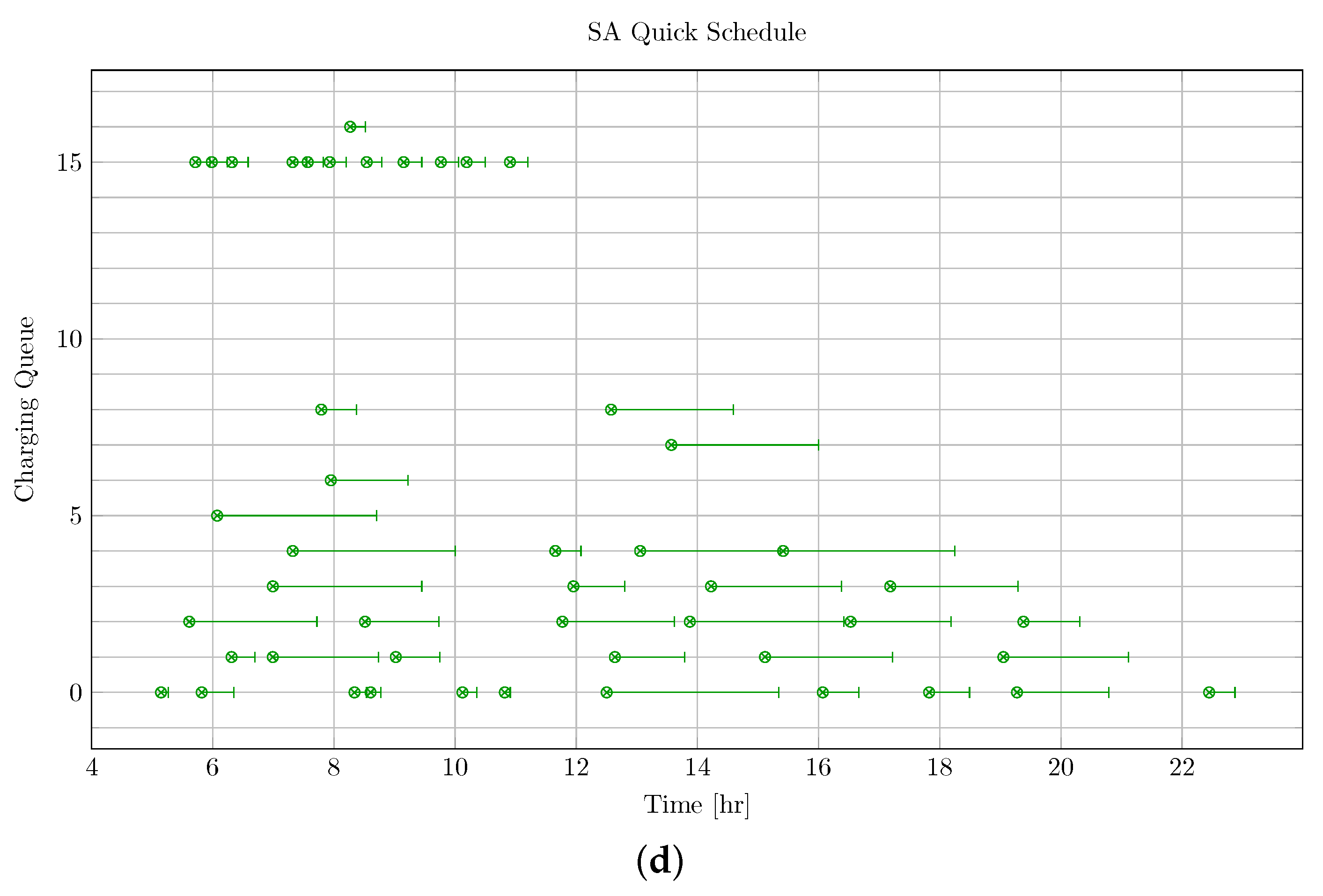
An example of the SA PAP algorithm was presented and compared against the BPAP, which acted as a baseline for the other schedule. Another threshold-based strategy called the Qin-Modified technique was also introduced as a means of comparing the schedules. The SA PAP was run utilizing two different neighborhood searching techniques named the “quick” and “heuristic” techniques, respectively. The quick SA’s objective was to randomly search a wide neighborhood while the heuristic technique was designed to incrementally search a neighborhood by randomly selecting a fast or slow charging queue and then stepping through the queues one at a time. The execution time compounds as the number of iterations in the cooling function increases as shown by the respective quick and heuristic execution times: 1532.8 s and 1916 s. The Qin-Modified strategy favored the use of fast chargers due to its inability to identify when demanding routes were on the horizon, whereas the other methods used fast charges sparingly. Particularly, the SA techniques favored higher number of slow chargers with longer charge durations in comparison to the BPAP.

Both of the SA techniques were unable to keep the SOC above the 25% SOC threshold, with SOC falling to 23.5% for the heuristic SA and 24.4% for the quick SA. Due to the minimum charge threshold being a soft constraint for the SA, the algorithm found other actions to be more favorable at the expense of moderately breaching the threshold. The Qin-Modified, on the other hand, had the SOC of one BEB fall to 0% SOC. The schedule that consumed the least amount of energy is the BPAP (4237.2 kWh) followed by the heuristic SA (4295.6 kWh). The difference between the two was about 8532.8 kWh. The quick SA energy consumption came in at a close third at 4428.7 kWh. Both the quick and SA techniques were able to significantly reduce the peak power demand, having peaks below 1200 kW. The BPAP and Qin both had peak power demands above 1800 kW. The best scoring schedule was the quick SA due to its significant reduction in demand cost, similar energy consumption as the heuristic SA and BPAP, and its small minimum SOC threshold deficit.

Future areas of interest are to introduce real-time capabilities to allow dynamic adaptation to the schedule. Furthermore, nonlinear battery dynamics are of interest to increase the fidelity of the charging model. In addition, methods to include uncertainty to the model, such as “fuzzifying” the initial and final charge times, are of interest to allow flexibility in the arrival and departure times.

References

1. Khan, S.; Maoh, H. Investigating attitudes towards fleet electrification—An exploratory analysis approach. Transp. Res. Part A Policy Pract. 2022, 162, 188–205. [Google Scholar] [CrossRef]
2. Li, J.Q. Battery-Electric Transit Bus Developments and Operations: A Review. Int. J. Sustain. Transp. 2016, 10, 157–169. [Google Scholar] [CrossRef]
3. Guida, U.; Abdulah, A. ZeEUS eBus Report# 2—An Updated Overview of Electric Buses in Europe; Technical Report 2; International Association of Public Transport (UITP): Brussels, Belgium, 2017. [Google Scholar]
4. Xylia, M.; Silveira, S. The Role of Charging Technologies in Upscaling the Use of Electric Buses in Public Transport: Experiences From Demonstration Projects. Transp. Res. Part A Policy Pract. 2018, 118, 399–415. [Google Scholar] [CrossRef]
5. Lutsey, N.; Nicholas, M. Update on Electric Vehicle Costs in the United States Through 2030. Int. Counc. Clean Transp. 2019, 12, 1–12. [Google Scholar]
6. Edge, J.S.; O’Kane, S.; Prosser, R.; Kirkaldy, N.D.; Patel, A.N.; Hales, A.; Ghosh, A.; Ai, W.; Chen, J.; Yang, J.; et al. Lithium ion battery degradation: What you need to know. Phys. Chem. Chem. Phys. 2021, 23, 8200–8221. [Google Scholar] [CrossRef] [PubMed]
7. Millner, A. Modeling Lithium Ion battery degradation in electric vehicles. In Proceedings of the 2010 IEEE Conference on Innovative Technologies for an Efficient and Reliable Electricity Supply, Waltham, MA, USA, 27–29 September 2010. [Google Scholar] [CrossRef]
8. Zhang, L.; Wang, S.; Qu, X. Optimal Electric Bus Fleet Scheduling Considering Battery Degradation and Non-Linear Charging Profile. Transp. Res. Part E Logist. Transp. Rev. 2021, 154, 102445. [Google Scholar] [CrossRef]
9. Duan, M.; Qi, G.; Guan, W.; Lu, C.; Gong, C. Reforming Mixed Operation Schedule for Electric Buses and Traditional Fuel Buses By an Optimal Framework. IET Intell. Transp. Syst. 2021, 15, 1287–1303. [Google Scholar] [CrossRef]
10. Rinaldi, M.; Picarelli, E.; D’Ariano, A.; Viti, F. Mixed-Fleet Single-Terminal Bus Scheduling Problem: Modelling, Solution Scheme and Potential Applications. Omega 2020, 96, 102070. [Google Scholar] [CrossRef]
11. Tang, X.; Lin, X.; He, F. Robust Scheduling Strategies of Electric Buses Under Stochastic Traffic Conditions. Transp. Res. Part C Emerg. Technol. 2019, 105, 163–182. [Google Scholar] [CrossRef]
12. Li, J.Q. Transit Bus Scheduling with Limited Energy. Transp. Sci. 2014, 48, 521–539. [Google Scholar] [CrossRef]
13. He, Y.; Liu, Z.; Song, Z. Optimal Charging Scheduling and Management for a Fast-Charging Battery Electric Bus System. Transp. Res. Part E Logist. Transp. Rev. 2020, 142, 102056. [Google Scholar] [CrossRef]
14. Wei, R.; Liu, X.; Ou, Y.; Fayyaz, S.K. Optimizing the Spatio-Temporal Deployment of Battery Electric Bus System. J. Transp. Geogr. 2018, 68, 160–168. [Google Scholar] [CrossRef]
15. Whitaker, J.; Droge, G.; Hansen, M.; Mortensen, D.; Gunther, J. A Network Flow Approach to Battery Electric Bus Scheduling. IEEE Trans. Intell. Transp. Syst. 2023, 24, 9098–9109. [Google Scholar] [CrossRef]
16. Mortensen, D.; Gunther, J.; Droge, G.; Whitaker, J. Cost Minimization for Charging Electric Bus Fleets. World Electr. Veh. J. 2023, 14, 351. [Google Scholar] [CrossRef]
17. Brown, A.; Droge, G.; Gunther, J. A Position Allocation Approach to the Scheduling of Battery-Electric Bus Charging. arXiv 2024, arXiv:2405.11365. [Google Scholar]
18. Zhou, Y.; Liu, X.C.; Wei, R.; Golub, A. Bi-Objective Optimization for Battery Electric Bus Deployment Considering Cost and Environmental Equity. IEEE Trans. Intell. Transp. Syst. 2020, 22, 2487–2497. [Google Scholar] [CrossRef]
19. Wang, X.; Yuen, C.; Hassan, N.U.; An, N.; Wu, W. Electric Vehicle Charging Station Placement for Urban Public Bus Systems. IEEE Trans. Intell. Transp. Syst. 2017, 18, 128–139. [Google Scholar] [CrossRef]
20. Yang, C.; Lou, W.; Yao, J.; Xie, S. On Charging Scheduling Optimization for a Wirelessly Charged Electric Bus System. IEEE Trans. Intell. Transp. Syst. 2018, 19, 1814–1826. [Google Scholar] [CrossRef]
21. Bie, Y.; Ji, J.; Wang, X.; Qu, X. Optimization of Electric Bus Scheduling Considering Stochastic Volatilities in Trip Travel Time and Energy Consumption. Comput.-Aided Civ. Infrastruct. Eng. 2021, 36, 1530–1548. [Google Scholar] [CrossRef]
22. Liu, T.; (Avi) Ceder, A. Battery-Electric Transit Vehicle Scheduling with Optimal Number of Stationary Chargers. Transp. Res. Part C Emerg. Technol. 2020, 114, 118–139. [Google Scholar] [CrossRef]
23. Qin, N.; Gusrialdi, A.; Paul Brooker, R.; T-Raissi, A. Numerical Analysis of Electric Bus Fast Charging Strategies for Demand Charge Reduction. Transp. Res. Part A Policy Pract. 2016, 94, 386–396. [Google Scholar] [CrossRef]
24. Jahic, A.; Eskander, M.; Schulz, D. Preemptive vs. non-preemptive charging schedule for large-scale electric bus depots. In Proceedings of the 2019 IEEE PES Innovative Smart Grid Technologies Europe (ISGT-Europe), Bucharest, Romania, 29 September–2 October 2019. [Google Scholar] [CrossRef]
25. Frendo, O.; Gaertner, N.; Stuckenschmidt, H. Open Source Algorithm for Smart Charging of Electric Vehicle Fleets. IEEE Trans. Ind. Inform. 2021, 17, 6014–6022. [Google Scholar] [CrossRef]
26. Zhou, G.J.; Xie, D.F.; Zhao, X.M.; Lu, C. Collaborative Optimization of Vehicle and Charging Scheduling for a Bus Fleet Mixed with Electric and Traditional Buses. IEEE Access 2020, 8, 8056–8072. [Google Scholar] [CrossRef]
27. Wang, Y.; Huang, Y.; Xu, J.; Barclay, N. Optimal Recharging Scheduling for Urban Electric Buses: A Case Study in Davis. Transp. Res. Part E Logist. Transp. Rev. 2017, 100, 115–132. [Google Scholar] [CrossRef]
28. Sebastiani, M.T.; Lüders, R.; Fonseca, K.V.O. Evaluating Electric Bus Operation for a Real-World Brt Public Transportation Using Simulation Optimization. IEEE Trans. Intell. Transp. Syst. 2016, 17, 2777–2786. [Google Scholar] [CrossRef]
29. Power, R.M. Large General Service. 2021. Available online: https://www.rockymountainpower.net/content/dam/pcorp/documents/en/rockymountainpower/rates-regulation/utah/rates/008_Large_General_Service_1_000_kW_and_Over_Distribution_Voltage.pdf (accessed on 3 April 2024).
30. Gendreau, M.; Potvin, J.Y. (Eds.) Handbook of Metaheuristics, 3rd ed.; Internationalseries in Operation Research & Management Science; Springer International Publishing: Berlin/Heidelberg, Germany, 2018. [Google Scholar] [CrossRef]
31. Press, W.H.; Flannery, B.P.; Teukolsky, S.A.; Vetterling, W.T. Numerical Recipes in C Book Set: Numerical Recipes in C: The Art of Scientific Computing, 2nd ed.; Cambridge University Press: Cambridge, UK, 1992. [Google Scholar]
32. Henderson, D.; Jacobson, S.H.; Johnson, A.W. The Theory and Practice of Simulated Annealing. In International Series in Operations Research and Management Science; Kluwer Academic Publishers: Dordrecht, The Netherland, 1989; pp. 287–319. [Google Scholar] [CrossRef]
33. Keller, A.A. Multi-Objective Optimization in Theory and Practice II: Metaheuristic Algorithms; Bentham Science Publishers: Sharjah, United Arab Emirates, 2019. [Google Scholar] [CrossRef]
34. Rutenbar, R. Simulated Annealing Algorithms: An Overview. IEEE Circuits Devices Mag. 1989, 5, 19–26. [Google Scholar] [CrossRef]
35. Zhang, D.; Liu, Y.; M’Hallah, R.; Leung, S.C. A simulated annealing with a new neighborhood structure based algorithm for high school timetabling problems. Eur. J. Oper. Res. 2010, 203, 550–558. [Google Scholar] [CrossRef]
36. Zhao, X. Simulated annealing algorithm with adaptive neighborhood. Appl. Soft Comput. 2011, 11, 1827–1836. [Google Scholar] [CrossRef]
37. Gurobi Optimization, LLC. Gurobi Optimizer Reference Manual; Gurobi Optimization, LLC: Portland, OR, USA, 2021. [Google Scholar]
Figure 1. Examples of different methods of overlapping. Space overlap: q k 1 > q i + 1 ψ i k 1 = 1 . Time overlap u k 2 < u j + s j σ k 2 j = 0 . Similarly, σ k 3 i = 0 .
Futuretransp 04 00049 g001
Figure 2. Graphical representation of the queue–time space. The shaded rectangles labeled A–D represent an example spatiotemporal plot of four scheduled BEBs. The vertical dashed lines represent the arrivial time, intitar charge time, final charge time, and the departure time for BEB D.
Futuretransp 04 00049 g002
Figure 3. Various schedules generated by the different frameworks. Panel (a) is the Qin-Modified schedule, (b) is the BPAP schedule, (c) is the heuristic SA schedule, and (d) is the quick SA schedule. The horizontal lines stemming from the nodes ending with a vertical tick indicate the charge duration for that particular visit.
Futuretransp 04 00049 g003aFuturetransp 04 00049 g003b
Figure 4. Power demand for each schedule over the time horizon. Panel (a) plots the power demand for the Qin and BPAP schedules, and (b) plots the power demand for the quick and heuristic SA schedules.
Futuretransp 04 00049 g004
Figure 5. Total accumulated energy consumed by the Qin-Modified, BPAP, quick, and heuristic SA schedules throughout the time horizon.
Futuretransp 04 00049 g005
Figure 6. Number of slow and fast chargers utilized in parallel over the time horizon. Panel (c) plots the slow charger count for the BPAP and Qin schedules and (d) plots the slow charger count for the quick and heuristic SA schedules. Similarly, (a) plots the fast charger count for the BPAP and Qin schedules and (b) plots the fast charger count for the quick and heuristic SA schedules.
Futuretransp 04 00049 g006aFuturetransp 04 00049 g006b