

Frustrated-Laser-Induced Thermal Starting Plumes in Fresh and Salt Water
by
 , , , and
Johnathan Biebighauser
1,
Johan Dominguez Lopez
2,
Krys Strand
3,
Mark W. Gealy
2 and
Darin J. Ulness
1,*
1
Department of Chemistry, Concordia College, Moorhead, MN 56562, USA
2
Department of Physics, Concordia College, Moorhead, MN 56562, USA
3
Department of Biology, Concordia College, Moorhead, MN 56562, USA
*
Author to whom correspondence should be addressed.
Liquids 2024, 4(2), 332-351; https://doi.org/10.3390/liquids4020017
Submission received: 14 December 2023
/
Revised: 2 March 2024
/
Accepted: 27 March 2024
/
Published: 8 April 2024
(This article belongs to the Special Issue Energy Transfer in Liquids)
Abstract
:The results of a photothermal spectroscopy technique that effectively images convective and conductive heat flow in liquids via a thermal lensing effect are described. Pure water; sodium chloride solutions at salinities of approximately 5, 15, 25, and 35 g/kg; and an artificial seawater of 35 g/kg were studied across a range of temperatures. This system was studied because of the importance of thermal pluming in seawater. ‘Frustrated’ thermal starting plumes were observed near the temperature of maximum density. The physical characteristics of these thermal starting plumes are reported.
1. Introduction
The current work employs a photothermal imaging technique recently developed by the authors [1]. This procedure is particularly useful for detecting convective heat flow in liquids arising from localized heating by a laser beam. In particular, thermal starting plumes in pure water and salt water were imaged and characterized in spite of the well-known fact that water is considered the worst of the common liquids for thermal lensing methodologies [2,3]. Thermal starting plumes are the initial part of the formation of a thermal plume originating from a heat source [4].
Of particular interest is the behavior of thermal starting plumes near the temperature of maximum density. Under these conditions, the buoyant force nearly matches the weight force. While there is potential for thermal pluming due to local heating, a plumehead does not rise rapidly or at all. It may, in fact, descend. These cases will be referred to here as ‘frustrated’ thermal starting plumes.
The temperature of maximum density in both pure and salt water has a critical effect on the coefficient of thermal expansion. In pure water, this temperature occurs near 4 °C. At this specific temperature, water molecules are arranged in a manner that maximizes their packing efficiency, resulting in the highest density achievable under normal atmospheric pressure. As the temperature decreases below 4 °C, the water molecules form a more ordered structure because of hydrogen bonding, resulting in a decrease in density.
One motivation for this work is to contribute to the understanding of temperature-driven convection near the temperature of maximum density in fresh water lakes during fall and spring turnover [5]. In temperate lakes, the phenomena of fall and spring turnover play a pivotal role in the maintenance of aquatic ecosystems. As the air temperature decreases in fall, the surface water cools, increases in density, and begins to descend, initiating a mixing process, which continues until the water column reaches a uniform temperature of approximately 4 °C. In the spring, the ice that formed on the surface over winter begins to melt, mirroring the thorough mixing that occurred in the fall. These seasonal turnovers are critical for redistributing oxygen from the surface to the lake’s depths, essential for the survival of various aquatic organisms, and for cycling nutrients from the bottom to the surface.
An additional motivation for this work is the importance of thermal plumes, both natural and human-made, in oceans and other bodies of water [6,7,8,9,10,11]. Understanding thermal plumes is crucial for comprehending various oceanic processes, including ocean circulation, heat transport, and their impact on climate systems [12]. Specific to pluming, mid-ocean ridges are a source of heat in the form of line plumes [12]. They also spawn volcanoes and hydrothermal vents. These offer places of distinctive chemical and biological activity [13]. To that end, the simulated seawater Instant Ocean® was included in the study in addition to sodium chloride solutions.
In the case of salt water, the presence of dissolved ions, primarily sodium (Na+) and chloride (Cl−) ions, alters the temperature of maximum density. This change occurs because the presence of salt disrupts the hydrogen-bonding network among water molecules, preventing them from forming the same dense structure observed in pure water. The temperature of maximum density is a linearly decreasing function of salinity, S, whose slope is greater in magnitude (more negative) than that for the melting point, which is also a decreasing function of salinity [14]. The temperature of maximum density reaches the melting point at a salinity of about [14] (the salinity units reported throughout this paper are grams of salt per kilogram of solution). For a recent thorough discussion of the importance of the effects and fluid mechanical treatment related to the frustrated thermal starting plumes discussed in the current paper, see the 2022 Ph.D. Thesis of Grace [15].
Following this Introduction, the various physical principles that underlie both the technique used in this work and the behavior of pure and salt water under the conditions of the reported experiments are discussed along with a semi-empirical model. This is followed by a description of the materials and methods. The results are then presented and discussed. The paper culminates with a conclusion and prospectus on future work.
2. Physical Principles
The primary physical phenomenon reported here is of thermal starting plumes. Following some discussion, this is then connected with the key physical principles that explain how the imaging technique works. These include thermal lensing and overtone/combination band absorption.
2.1. Thermal Plumes
This study investigates the dynamics of thermal starting plumes generated through rapid laser-induced heating. Thermal plumes, often referred to as convective plumes, represent vertical fluid motions driven by temperature variations, encompassing both heat and mass transfer. The exploration of thermal plumes dates back to the middle 1950s and early 1960s [16,17] with laser-induced thermal plumes being observed shortly thereafter [18]. The definitions employed in this paper for thermal plumes align with Turner’s seminal work on buoyancy effects in fluids [4].
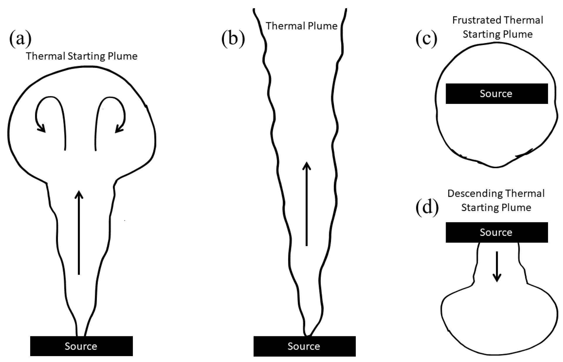
Thermal starting plumes are transient phenomena that occur at the onset of heating. A schematic representation of a thermal starting plume is presented in the leftmost caricature in Figure 1. When a fluid experiences initial heating, it generates localized buoyant forces, which propel a plume upwards. These starting plumes are known for their rapid formation and the initial momentum they acquire from the heat source, a laser beam in this case. As the heated fluid ascends from its sustained source, it gives rise to a well-defined plumehead and a columnar structure termed the conduit. Collectively, the thermal starting plume is distinguishable from its surroundings due to a sharp spatial temperature gradient. The structure of a thermal starting plume is illustrated in Figure 2. Thermal starting plumes play a pivotal role in initiating the convection process, setting the stage for the subsequent formation of more sustained and steady-state thermal plumes [4,19,20,21].
As long as the heat source persists, the thermal starting plume ultimately becomes a thermal plume, as depicted in the middle caricature of Figure 1. These are steady-state structures characterized by sustained upward motion due to continuous heating from below. The present analysis primarily focuses on the transient phase of thermal starting plumes, and the steady-state case falls outside the scope of this study. If the heat source is not sustained, but rather, persists for only a short time, thermals are produced. These are isolated, buoyant parcels of fluid that rise due to heating from a localized source. Unlike continuous thermal plumes, thermals are intermittent and can be thought of as ‘puffs’ of heated fluid that detach and ascend independently. While they are not the focus of this work, they are related to the time when the laser source is shut off. These will be referred to here as “thermal ending plumes”.
In this study, special emphasis is placed on investigating the behavior of thermal starting plumes that occur near the temperature of maximum density. At such a temperature, the net force of buoyancy and weight acting on the fluid is greatly diminished, approaching zero. While the potential for thermal pluming due to localized heating still exists, the behavior of these plumes takes on a distinct nature. Instead of rising rapidly, as typically observed in conventional thermal starting plumes, these plumes are frustrated in their ascent, and sometimes, they do not ascend at all. In fact, they may stall completely or even exhibit a downward motion. These frustrated thermal starting plumes are represented in caricature on the right of Figure 1. The frustrated thermal starting plume dynamics is distinct from the case of highly viscous liquids, such as glycerol or silicone oil. In those cases, the viscosity prevents convection in the form of a thermal starting plume. Heat is dissipated symmetrically via conduction. Such a comparison will be discussed in the Section 4.
Entrainment
Entrainment is a central process in the dynamics of all thermal plumes, including thermal starting plumes, involving the drawing of fluid layers adjacent to the conduit’s layers into the plume through frictional forces [22]. Entrainment plays a critical role in determining the growth, shape, and eventual transition of the thermal starting plume into a steady-state thermal plume [4]. The velocity differential at the boundary layer generates eddies, facilitating the mixing of ambient fluid into the plume. As the plume entrains more surrounding fluid, its mass increases, potentially slowing its ascent. However, the additional entrained fluid also brings added buoyancy, further promoting upward plume movement. The balance between these factors represents a key aspect of the dynamics of thermal starting plumes. Modeling entrainment in thermal starting plumes often involves a combination of buoyancy-driven flow equations and turbulence modeling. One commonly employed framework is the Boussinesq approximation, which simplifies the Navier–Stokes equations for buoyancy-driven flows. In this model, fluid density is assumed to be constant except where it appears in buoyancy terms, allowing linearization of density variations due to temperature. In terms of equations that yield to analysis, the prevailing theory is that of Morton, Taylor, and Turner called MTT theory [4,16,17,19]. This is still the one used today [23,24,25,26] and has recently been extended by Wise and Hunt for wall and (more related to the current work) line plumes [27]. However, because of the additional entrainment into the laser region itself, the current authors suspect that the conditions of the photothermal method used in this work do not completely align with the assumptions of MTT theory. A full computational fluid dynamics investigation could be fruitful, but is beyond the scope of this paper.
2.2. Thermal Lensing
Photothermal spectroscopies, encompassing a range of non-destructive analytical methods, utilize the conversion of light energy, typically emanating from laser sources, into thermal energy within a sample [28,29,30,31,32]. Localized laser-induced heating gives rise to spatial gradients and temporal temperature variations within the sample. Detection of these gradients can be achieved indirectly through various means, such as monitoring changes in the refractive index, thermal expansion, or the generation of acoustic waves, depending on the specific photothermal method utilized. The principal branches of these methods encompass photoacoustic spectroscopy, thermal lensing, and photothermal deflection spectroscopy. The method used in the current work is a combination of thermal lensing and photothermal deflection.
Thermal lensing, originating in the mid-1960s with pioneering work by Gordon et al. [33], and further developments in the early 1970s, revolves around the creation of a thermal lens within the sample due to uneven heating induced by a focused laser beam [28,31,32,34,35,36,37]. This phenomenon arises from a change in the refractive index of the medium, which can be detected using a probe beam. The exceptional sensitivity of this method makes it particularly effective for analyzing transparent liquids. Photothermal deflection spectroscopy, also known as the mirage effect, involves the use of an excitation beam to heat a sample, generating a temperature gradient that modifies the refractive index of the surrounding medium [38,39]. The resulting deflection of a probe beam is measured to assess the sample’s absorption.
The approach discussed here integrates elements of both thermal lensing and photothermal deflection in a novel manner. In these experiments, the excitation beam remains collimated as it passes through the sample cuvette, instead of being focused to create a cylindrical lens. Consequently, the probe beam encounters a cylindrical region perpendicular to its propagation direction. Because the refractive index within the heated cylindrical region is lower, the light diverges. This leads to a relative increase in light intensity at the edges of the cylinder compared to the background, while the central cross-section of the cylinder experiences a relative decrease in light intensity. Consequently, both the rising plumehead and the plume source cast ‘shadows’ with well-defined bright outlines. The divergent nature of the probe beam allows for the illumination of the entire length of the excitation beam within the sample, as well as a region several mm above and below, enabling the observation of the convective flow from the excitation beam. This methodology shares similarities with the approach taken by Longaker and Litvik in their 1969 publication, where they employed a similar excitation-perpendicular-to-probe beam arrangement with a corresponding camera setup [40].
Decades ago, Lee and Albrecht introduced a valuable classification scheme for spectroscopic methods, focusing on the nature of the interaction between light and matter [41]. In this context, spectroscopic techniques that involve light–matter interactions that survive cycle-averaged energy transfer are categorized as active spectroscopies. Conversely, those techniques in which the light–matter interaction does not persist through cycle averaging are labeled as passive spectroscopies. While this classification scheme is particularly advantageous for organizing nonlinear spectroscopies, it also finds relevance in understanding linear processes. In the context of this work, refraction is an example of a passive process, while (linear) absorption is an example of an active process.
In many cases, the interaction of visible or near-infrared light with clear molecular liquids is considered passive. This is because the process is predominantly governed by refractive behavior, which is controlled by the refractive index of the specific liquid. However, in photothermal methods like traditional thermal lensing, and the one employed in this study, there exist both active and passive components. While only a relatively small fraction of the incident light is absorbed, such absorption plays a crucial role in generating localized heating within the sample. The passive component of photothermal techniques involves exploiting the refractive index gradients that arise as a consequence of this localized heating. Consequently, the strength of the observed photothermal signal, denoted as , is directly proportional to the absorptivity (), the temperature-dependent refractive index change (), and the power of the excitation laser (), as expressed by the equation:
A significant portion of the existing research on photothermal phenomena has primarily concentrated on thermal conduction. However, more recent investigations led by research groups including Goswami et al. [42,43,44,45,46] and Khabibullin and Wang [47,48] have studied the role of thermal convection in the context of thermal lensing. This recent body of work expands upon prior research, including the earlier contributions made by Buffett and Morris [49].
2.2.1. Overtone/Combination Band Absorption
In the mid-1970s, Long and colleagues explored the phenomenon of absorption in thermal lensing within the framework of a vibrational local mode model [37]. This conceptual foundation was further developed in the early 1980s by Swafford et al., who explored the details of energy absorption from the excitation beam by molecular liquids [32,50,51]. Their investigations revealed that a portion of the excitation beam’s energy is absorbed into vibrational overtone bands or combination bands that involve overtone bands along with other local or normal modes.
The crucial insight gleaned from these findings is that the behavior of local modes plays a pivotal role in determining the extent of light absorption and, consequently, the degree of local heating. This fundamental principle underpins photothermal techniques as valuable tools in chemical analysis. Of relevance to the current study is how this manifests in water, which has only O–H stretches and bends. The particular excitation beam used in this work is primarily absorbed by the third harmonic of the O–H stretches. Work by Tran et al. shows a broad absorption peak for pure water near 970 nm with a gradual shoulder extending well past the 1030 nm used in this study [52]. For this work, the absorption coefficient for this mode is small and, in conjunction with other properties of water, particularly its relatively large thermal conductivity and its relatively small rate of change of index of refraction with temperature, leads to rather weak signals.
3. Materials and Methods
In this section, the experimental setup is detailed, the sample preparation is described, and the data analysis procedure is outlined.
3.1. Experimental Setup
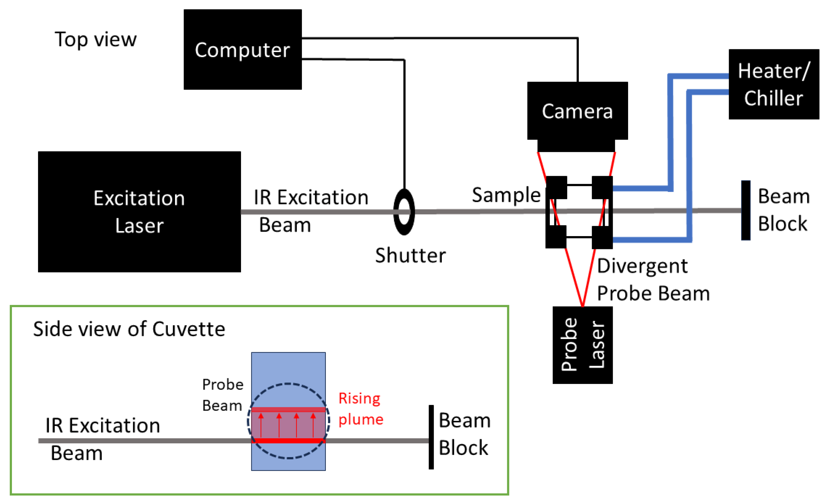
The experimental setup, as illustrated in Figure 3, includes an excitation laser, the QSL103A Q-Switched Picosecond Microchip Laser System by Thorlabs, Newton, NJ, USA emitting light at a 1030 nm wavelength. This laser generates pulses approximately 500 ps long at a repetition rate of approximately 9 kHz, and its beam predominantly follows a Gaussian spatial distribution. Note that, given the timescales involved in the photothermal processes (on the order of seconds), the laser’s operation resembles that of a continuous wave source.
The power reaching the sample, which was largely unabsorbed, was measured using the PM100D Digital Optical Power and Energy Meter from Thorlabs, equipped with an S140C powerhead. This meter has an uncertainty of about 7% at 1030 nm, as specified in the product datasheet. Additionally, it was observed that approximately 7% of the laser’s power was reflected off the front surface of the cuvette. Therefore, the power values reported in the subsequent Section 4 were adjusted to account for 93% of the initial measurements directly from the laser. A computer-controlled solenoid-actuated shutter enabled the recording of the background (shutter closed), active (shutter open), and recovery (shutter closed) phases during the experiment.
The probe beam was generated by a low-power diode laser from HiLetgo, operating at a 650 nm wavelength. This laser was placed within a passive aluminum heat sink and connected to a potentiometer, allowing for the adjustable irradiation of the sample. While the emitted powers had minimal impact on the sample, this adjustability was crucial for fine-tuning the camera’s exposure settings.
The imaging system utilized an Arducam Camera equipped with a 5-megapixel Omnivision OV5647 sensor. Although capable of operating at a resolution of 1080 p, the camera was configured to function at pixels to achieve a higher frame rate, which was advantageous for capturing dynamic processes in the experiment with greater temporal resolution. The recorded video was encoded in raw .h264 format. Because this format lacks timestamp information in individual frames, time calibration was obtained by recording ten, 10.0 s videos and averaging the total number of frames collected. This process established a time calibration of seconds between successive frames. Monitoring the software’s timing of the shutter opening revealed an estimated timing jitter of fewer than 2 frames. Space calibration of the video data was achieved by introducing a 1.25 mm obstruction at the sample’s position, creating a shadow visible to the camera. Due to the inherent diffraction effects, a subjective assessment was made to identify which pixels corresponded to the obstruction’s edges. The spatial calibration value was 3.54 µm per pixel.
A Raspberry Pi 4 microcomputer was responsible for coordinating the operation of the shutter mechanism and acquiring data from the camera. The Raspberry Pi 4 ran custom-designed software tailored specifically for this experiment (https://github.com/ulnessd (accessed on 14 December 2023)).
3.2. Sample Preparation
The sample was placed in a 1 cm × 1 cm fluorimeter cell, which was set into a brass jacket built in-house. Ethylene glycol flowing through the jacket was heated/cooled using an FTS model RS33AL10 heater/chiller. Sample temperatures compared to reservoir temperatures were calibrated from 0 °C to 70 °C. The heating/chilling was regulated to ±0.5 °C. For temperatures below 10 °C, argon flowed over the cuvette to prevent condensation.
The water used in this work was obtained from an in-house reverse-osmosis system. The sodium chloride was obtained from Fisher Scientific and used without further purification to prepare salinity values of , , , and . Instant Ocean® is a fairly complete seawater substitute used to house marine animals. The composition of Instant Ocean® is listed in Table 2 of Reference [53]. There is considerable agreement with the ion concentrations compared to actual seawater reported in Table I of Wiesenburg and Little [14]. In particular, the top six ions by composition are chloride, sodium, sulfate, magnesium, calcium, and potassium, and they are represented in Instant Ocean® within 1–2% of that for seawater. These six ions constitute 99.35% of the ions in real ocean water. Missing from Instant Ocean® are the many trace elements found in the oceans (see Table II of Reference [14]. Instant Ocean® was prepared at .
3.3. Data Collection
For each sample and temperature, 20 runs were recorded sequentially with either a 30 s (≥20 °C) or 90 s (≤15 °C) rest interval between runs, i.e., a given run began its background phase of 30 s or 90 s after the recovery phase of the previous run. During data analysis, careful observation for systematic trends across the 20-run set was made to ensure that the sample was not starting each run at a warmer temperature than the previous.
3.4. Data Analysis
The data analysis in this experiment was conducted using a set of custom-written programs https://github.com/ulnessd (accessed on 14 December 2023). The data processing involved three main steps. First, the video data were processed. Second, dynamic information related to the starting plumes was extracted and combined with relevant physical data from the existing literature. Finally, the dynamic and physical information were plotted and interpreted.
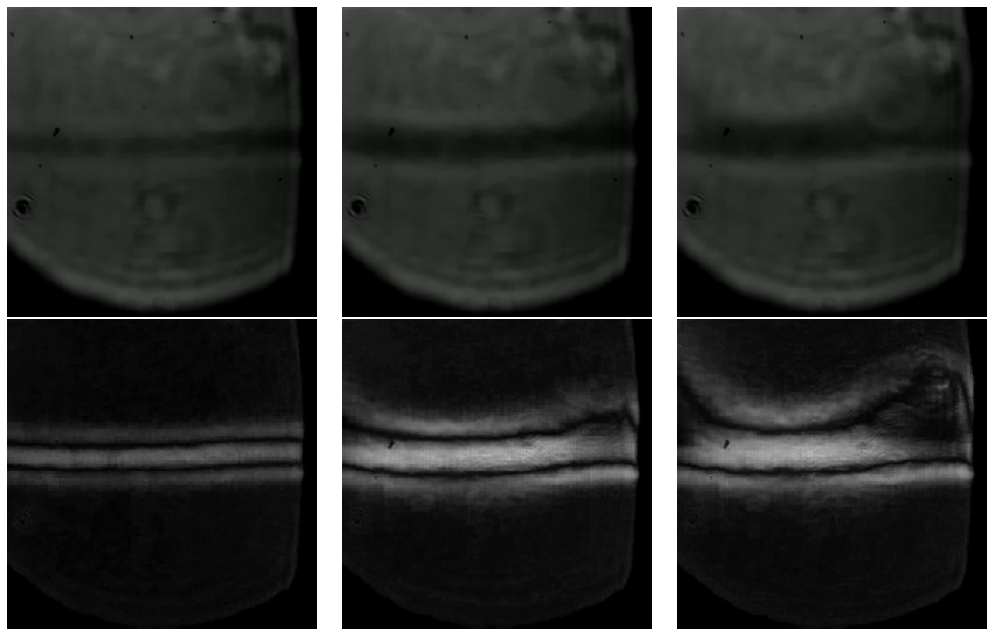
The video-processing phase followed a structured procedure. Initially, the 20 individual .h264 files were averaged and converted into a single .avi file, which is referred to as the raw sample video and serves as the initial data for the given sample liquid. The top row of Figure 4 shows an example of this for water at °C. There, single frames are shown at times s, s, and s. During the first 2 s, the laser was blocked by the shutter; therefore, the images show the raw visual field at s, s, and s after the light first reached the sample. In the image, the laser position is about half-way up the frame and appears as a dark horizontal region. It is dark relative to the spatial background because the heated volume had a lower index of refraction, causing light to diverge from this region. Although somewhat difficult to see, there are two regions that are slightly brighter than the spatial background directly above and below the heated region. Finally, the curved structure at the bottom of the frame is the edge of the probe beam and is of no physical relevance.
Subsequently, a new .avi video was generated by averaging the first 120 frames (equivalent to 1.23 s) of the temporal background from the raw sample video and subtracting this averaged background from all frames in the raw sample video file. The absolute value of the subtracted difference then becomes an individual frame in this second video file referred to as the background-subtracted video. The bottom row of Figure 4 shows the precise frame in the subtracted video as its corresponding raw video. This process enhances the visualization of both the transient and stationary components of the material’s response. Specifically, the transient feature corresponds to the thermal starting plume, while the stationary component represents the region where the laser interacts with the sample, referred to as the plume source.
For static visualization of the video data in the form of a single figure, the averaged background-subtracted video was compressed into a heatmap. The heatmap image was created by integrating each row in a given frame to produce one individual column in the heatmap. The presentation and analysis of the heatmap representations make up the bulk of the Section 4. All the video files can be found at https://www.darinulness.com/research/data/frustrated (accessed on 14 December 2023).
3.5. Artificial Intelligence
It is appropriate to acknowledge the extensive use of OpenAI’s ChatGPT 4.0 in assisting with the development of the programs to acquire and analyze the data [54]. Use in writing was minimal and limited to paraphrasing previous writings from the authors and producing references in the correct format. Sundry use as background and/or support of the authors included collecting and organizing the papers both used and not used based on the AI’s understanding of the abstracts.
4. Results and Discussion
Results for pure water, an artificial seawater, and several salinities of salt water at a variety of temperatures are presented and discussed.
4.1. Pure Water
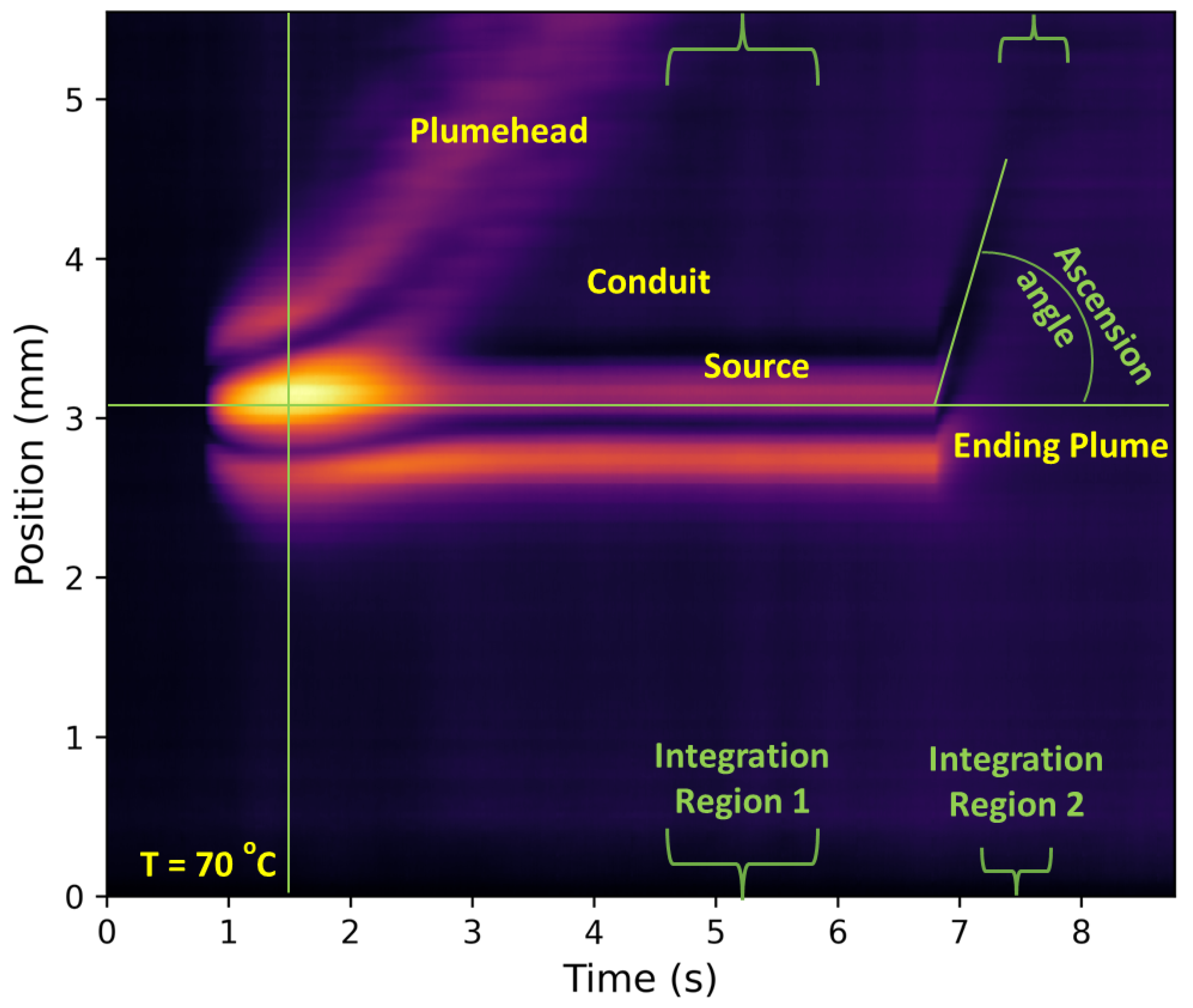
As mentioned at the end of the previous section, the results are compressed into heatmaps. By way of example, the heatmap for pure water at 70 °C is shown in Figure 5. This example offers an illustrative representation of thermal plume dynamics within which several distinct features are apparent. Notably, there is a visually pronounced rising plumehead and source, which manifest as prominent regions of elevated temperature. In contrast, the conduit is less discernible, primarily due to a less abrupt temperature gradient when compared to the leading edge of the plumehead and the laser-heated region. The excitation laser is positioned along the horizontal green line. This line serves as the reference for kinetics traces in subsequent analyses. Beneath this, one observes a significant feature resulting from the thermal lens effect, causing light to bend outward from the cylindrical region. Furthermore, the vertical green line indicates the point of plumehead formation, or the time to form the plumehead, . Upon shutter closure, the heated fluid within the laser region rapidly ascends, marking the initiation of a thermal ending plume. The ascension angle, , is denoted by an angled green line, while curly brackets delineate integration regions encompassing asymmetry arising from convection effects. This heatmap provides valuable insights into the complex dynamics of thermal plumes under the specified conditions.
4.1.1. Heatmap Representation of Thermal Starting Plumes
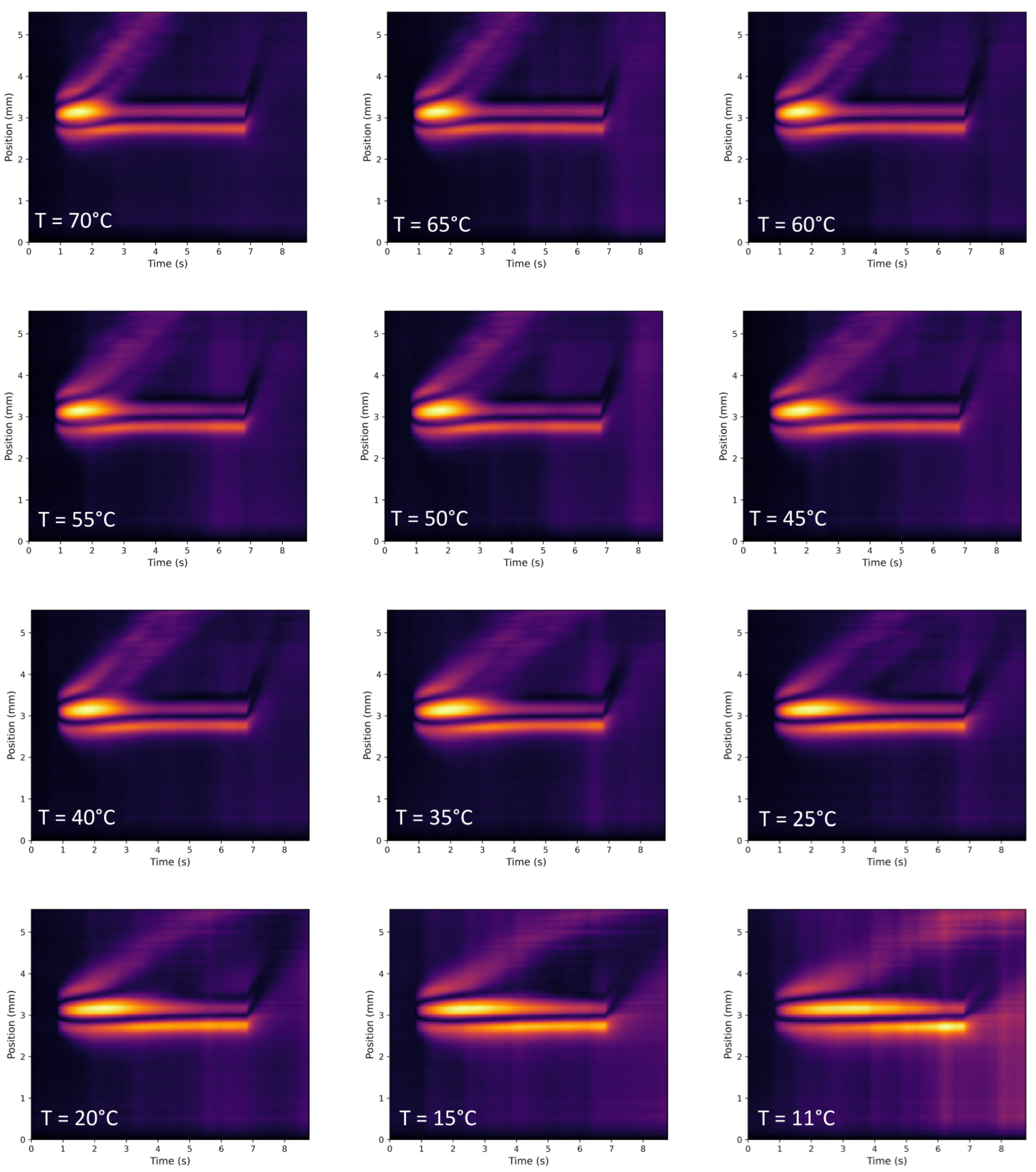
Figure 6 shows heatmaps for pure water at varying temperatures ranging from 11 °C to 70 °C. In this examination of the heatmaps, distinct temperature-dependent features become apparent. As illustrated in Figure 6, the thermal plume dynamics exhibit notable variations with changing temperature. A key observation is the diminishing time required for plumehead formation and the accelerated ascent of the plumehead as the temperature increases. While the signal-to-noise ratio exhibits a decline at lower temperatures, it remains clearly perceptible above the background level.
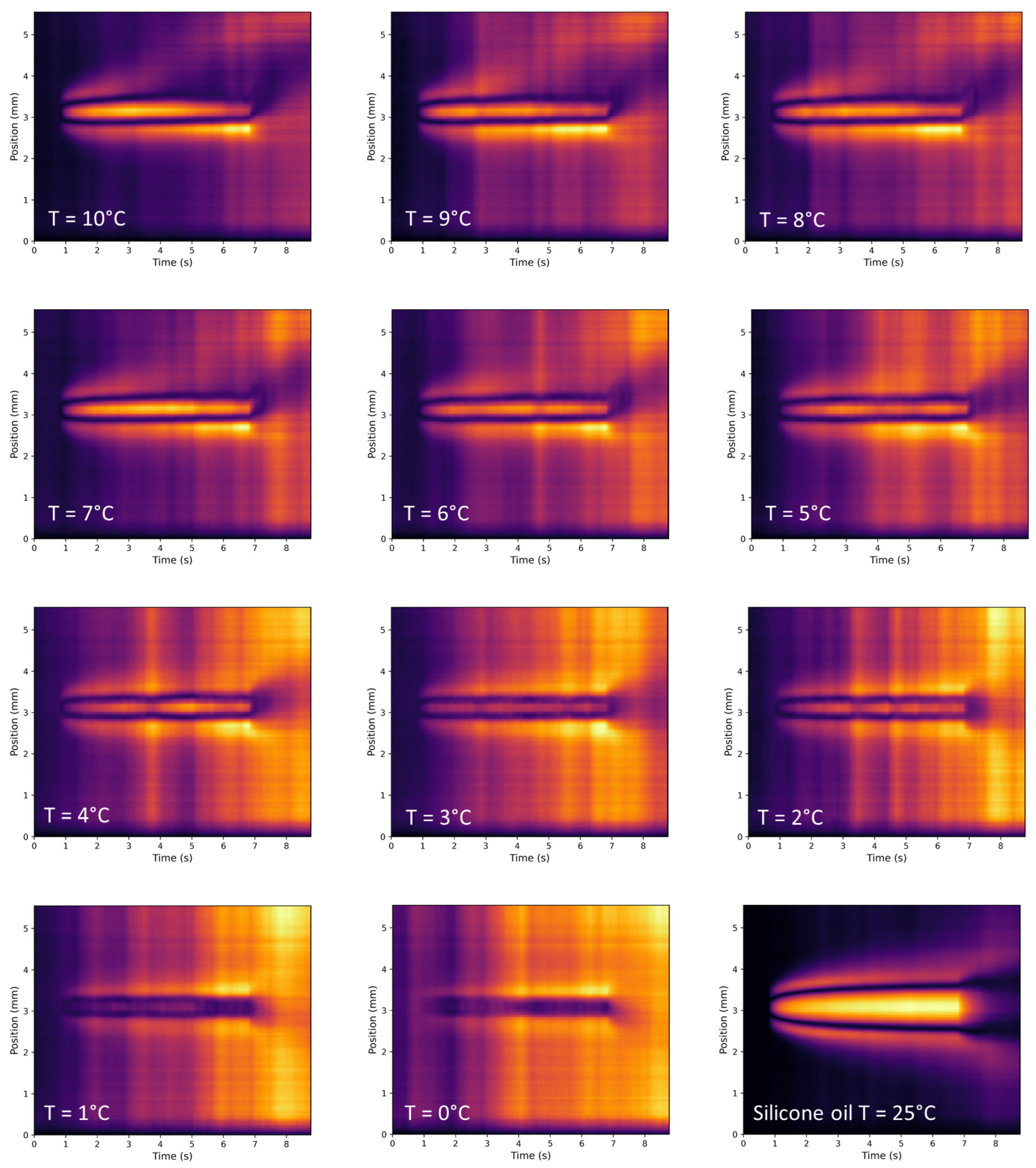
In contrast, the investigation of the heatmaps for temperatures ranging from 0 °C to 10 °C reveals a more rapidly changing set of characteristics (Figure 7). At these lower temperatures, the signal-to-noise ratio exhibits significant degradation, leading to reduced clarity in the observed phenomena. Figure 8 shows a plot of the total integrated signal for each of the temperatures studied.
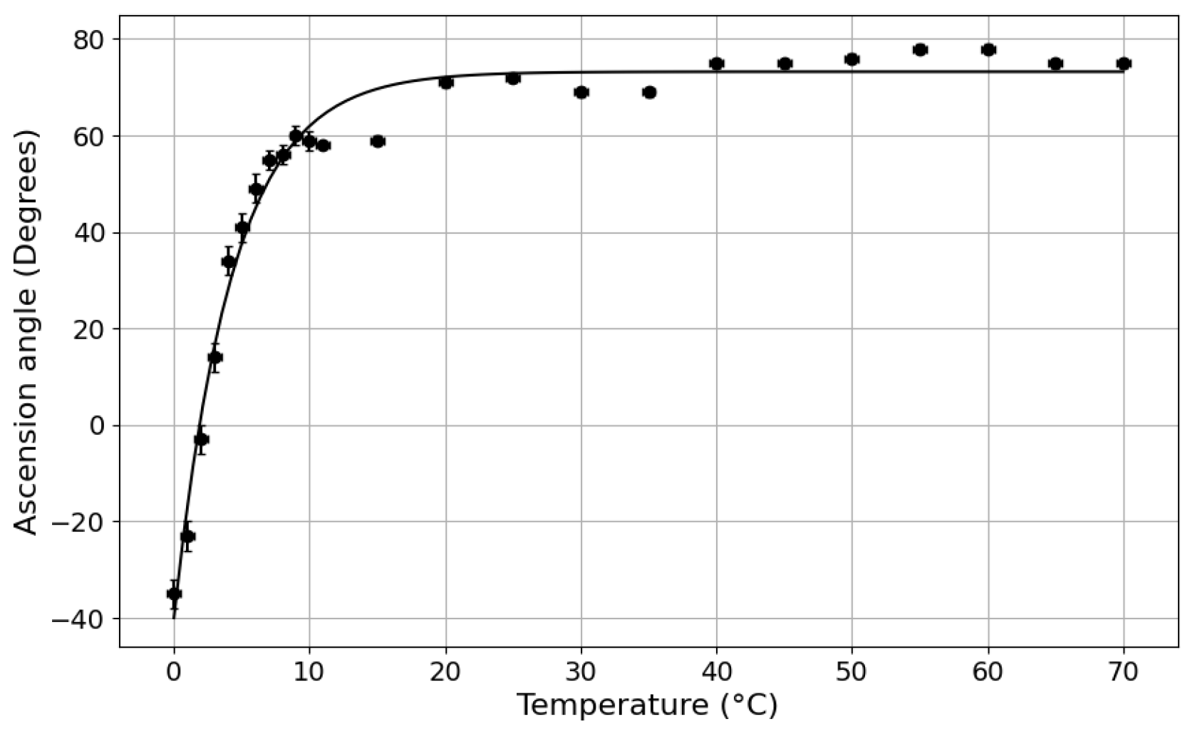
Despite the challenging noise conditions at low temperatures, certain features remain discernible. In particular, a rising plumehead is evident, persisting down to 7 °C. A central observation to the main theme of this paper is the rapid decrease in the ascension angle of the thermal ending plume in contrast to the nearly constant ascension angle observed in the higher temperature range depicted in Figure 6 (the ascension angle is plotted in Figure 9). Furthermore, indirect evidence of the transition from ascending frustrated starting thermal plumes to descending frustrated thermal starting plumes is discernible through an assessment of the relative intensities of light accumulation above and below the laser position, as observed in Figure 6.
Serving as a counterexample, the heatmap for silicone oil is shown in the bottom right panel of Figure 7. One sees here a similar case to the fully frustrated thermal starting plume of water at about 2 °C, albeit a much stronger signal. Convection via thermal pluming also does not appear for silicone oil, but for a different physical reason. The silicone oil is indeed heated in the laser region, and that region is indeed less dense than the ambient fluid. However, because of the very high viscosity of silicone oil, nearly 10,000-times that of water, the viscous drag force effectively stops ascension. For the frustrated thermal starting plumes of water, there is the potential for thermal starting plumes in terms of viscosity, but because the buoyant force matches the weight force, there is no net movement regardless of viscosity.
The transition observed at low temperatures, characterized by a shift from a bright central line (representing the laser position) to a dark central line, warrants the following discussion. A comparison between the heatmaps for 6 °C and 0 °C highlights this transition. This phenomenon arises due to the nature of the heatmaps, which depict the absolute difference from the background. For low temperatures, the thermal lens effect causes the deviation of light from the laser path, resulting in reduced light intensity within the laser region. Given that the background signal is heavily averaged (over 120 frames), its contribution to noise in the heatmap is relatively diminished compared to the individual frames from which it is subtracted. Consequently, noise fluctuations in the laser region exhibit a lower magnitude in comparison to the rest of the visual field, manifesting as a darker central line. Conversely, noise becomes more pronounced in the regions directly above and below the laser position, resulting in brighter lines in the heatmap.
4.1.2. Semi-Empirical Model
The total signal strength as a function of temperature and Equation (1) can be viewed in the context of a very simplified chemical equilibrium model (dots representing hydrogen bonding):
Using the local mode/combination band model discussed above, the signal strength is determined by the density of ‘free’ (not involved in a hydrogen bond) O–H, [55], where Y is the percent population of free O–H. Unfortunately, while in principle, it is possible to construct a chemical equilibrium model to obtain thermodynamic information, in practice, these thermodynamic values as fit parameters carry too much variance, rendering them useless. Instead, one must settle for a semi-empirical model that fits the lensing-corrected signal strength (), discussed below, to the Hill equation [56]. These data reveal the ultimate effect of extended water structures on heat transport. Studies of the extended network of water near and below freezing have been performed by Magazú et al. in the late 1980s through the mid-1990s [57,58,59] and are relevant to the free OH model of Fang and Swofford [50].
Reconsidering Equation (1), and hiding the constant laser power, but exposing the source of the absorption, one expresses
where is the molar absorptivity of free O–H and the constant laser power has been absorbed in the proportionality. Rearranging gives
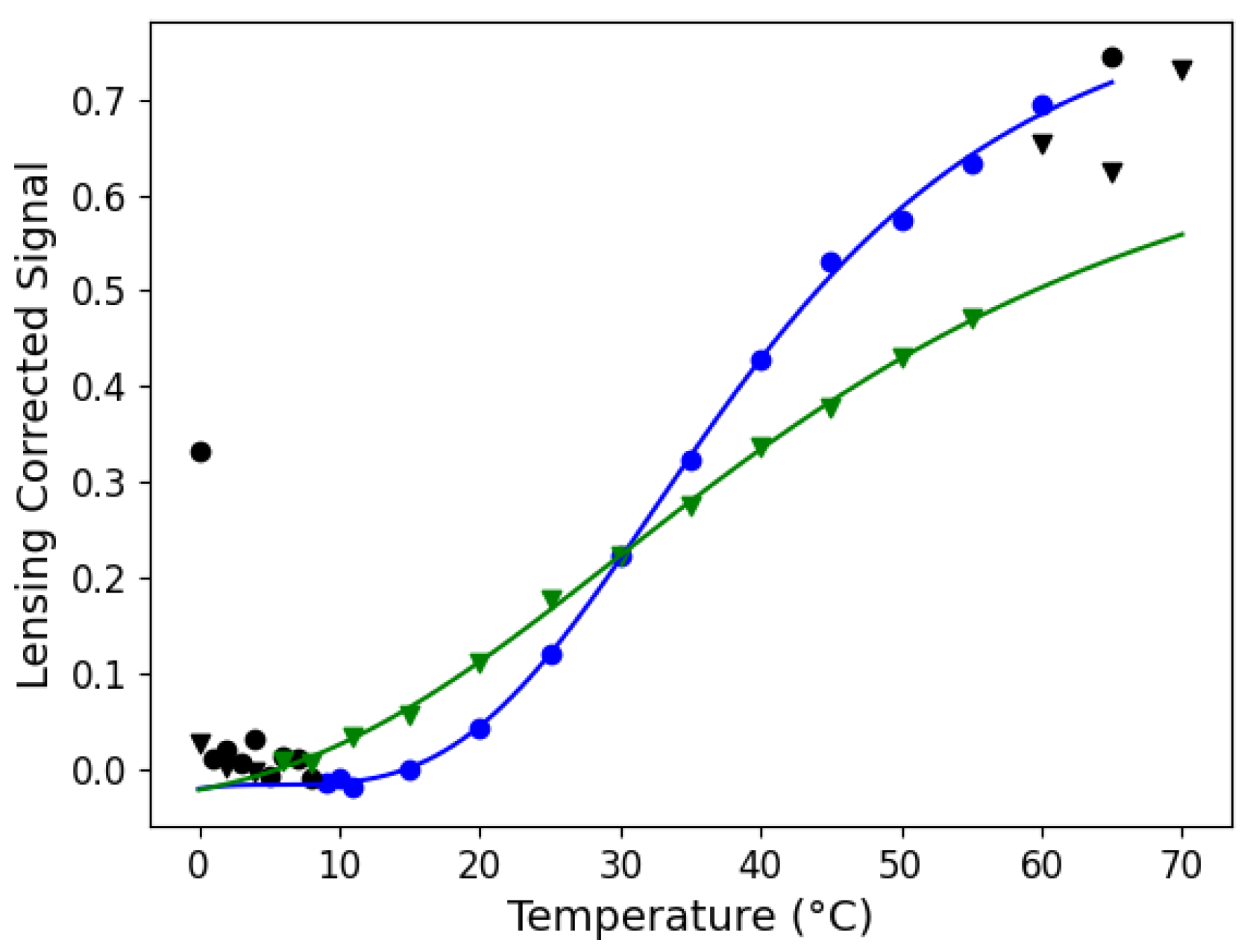
The measured data for are collected in Figure 8. As discussed in Section 3.4, Data Analysis, each datum represents a 20-run average. Individual error bars are not generated because the lens-corrected total integrated signal was determined from the averaged data set. However, the relative standard deviation is estimated at 2.25% based on an approximate 10% standard deviation of the individual runs, and thus scaled by a factor of . These data are fit to the Hill equation with Hill coefficient :
The Hill coefficient is an empirical measure of cooperativity/anti-cooperativity with representing cooperativity and representing anti-cooperativity ( recovers a neutral Langmuir behavior). The visual quality of the fit is reasonable for values of between and , but appeared to be the best. The blue and green curves in Figure 8 show the fits of for pure water and Instant Ocean®, respectively. It is also important to note that one must not read too much into the actual values of the parameters as the Hill equation is purely empirical [56]. This fact, combined with the chemical model above, is the rationale for calling the model semi-empirical.
Although the Hill equation is used to fit cooperative ligand binding systems, the analogy here is that the ligand concentration is replaced with temperature. Temperature is serving as a surrogate for bound and unbound waters per Equation (2).
The ‘cooperativity’ stems from the various states of hydrogen bonding that water can be in as indicated in the simplified chemical reaction of Equation (2). At low temperatures, the equilibrium shifts to the right, quenching the signal, because the O–H stretch is both diminished and shifted [55]. Conversely, at high temperatures, the equilibrium shifts to the left, liberating O–H bonds and, thus, enhancing the signal. This behavior is readily apparent upon inspection of Figure 6 and Figure 7.
4.1.3. Asymmetry in Steady-State and Thermal Ending Plumes
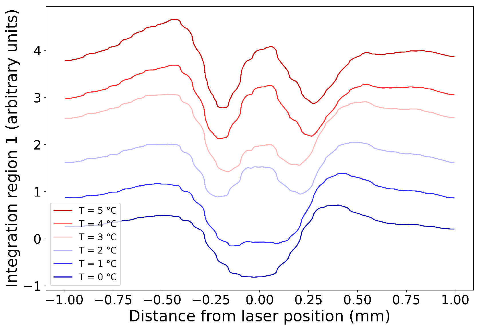
There is a visually apparent asymmetry as one views integration region 1 from Figure 5. For ascending thermal starting plumes, there is a brighter streak below the central streak of the laser region. The converse is true for descending plumes in which the streak above the laser line is brighter. The reason for this is that the conduit in either case acts to reduce the spatial temperature gradient, thereby diminishing the thermal lensing effect.
There is a way to better discern the asymmetry, which is by plotting the integrated signal strength within integration region 1 from Figure 5. The graphs for these values for temperatures near the temperature of maximum density are collected in Figure 10. The graph of Figure 10 shows a comparison between temperatures of 0 °C and 5 °C. At 0 °C, the peak on the positive side of zero (the laser position) exceeds that on the negative side. Visual scrutiny of the asymmetry observed in the peaks on the left and right sides suggests the occurrence of the fully frustrated thermal starting plume to transpire between 1 °C and 2 °C. The authors estimate the fully frustrated plume occurs at °C.
Advantageously, this allows for an estimate of the laser-induced temperature increase. By utilizing the empirical formula of reference [14] and solving for the temperature in the laser region, , and subtracting the temperature of the bulk, , give °C.
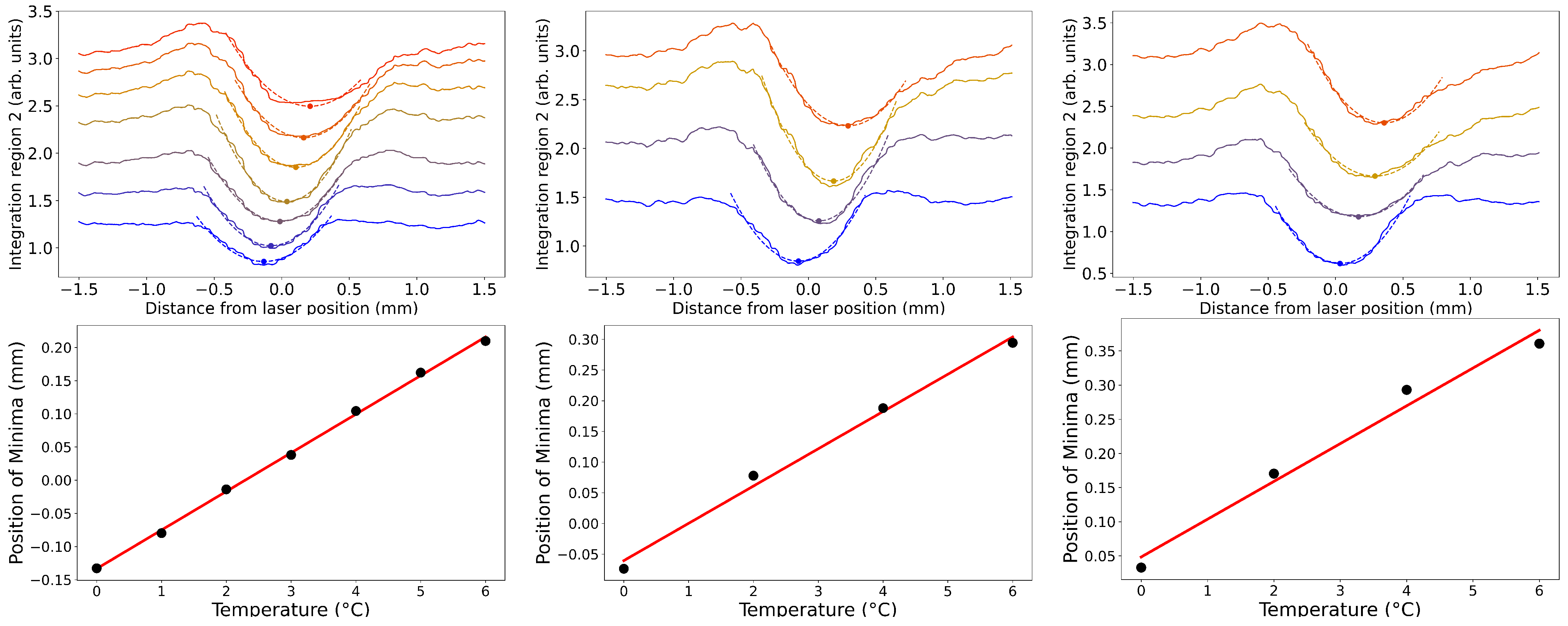
The left panel of Figure 11 illustrates the thermal ending plumes across a temperature range from °C to °C. The observations reveal a transition from an ascending frustrated thermal starting plume at °C to a fully frustrated thermal starting plume occurring near °C, followed by a descending frustrated thermal starting plume at °C. To quantify these observations, quadratic functions were fit to the troughs within a narrow range near their minima. The minima extracted from these fits were then plotted against temperature, as shown in the right-hand graph. The trend is remarkably linear, giving insight into the temperature-dependent behavior of thermal starting plumes near the temperature of maximum density.
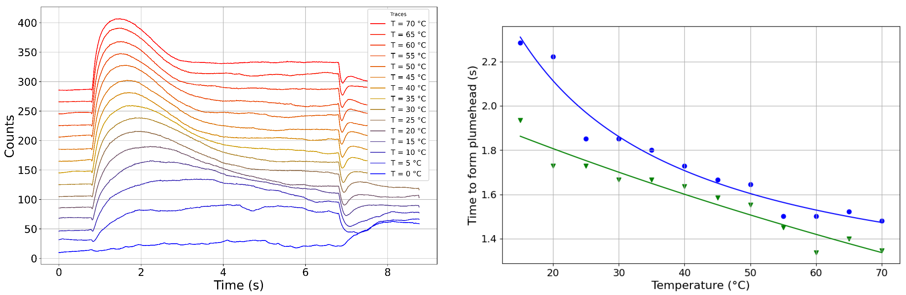
The kinetics traces at the position of the laser (green horizontal line in Figure 5) are shown for water in the left graph of Figure 12. As temperature is reduced, the peak in the traces grows smaller and wider and occurs later. This is consistent with the reduced signal due to increasing hydrogen bonding, as well as an increase in viscosity as temperature decreases. The time of the peak is the time to form the plumehead [21].
The time to form the plumehead is plotted for both water (blue) and Instant Ocean® (green) in the right graph of Figure 12. Notably, water follows what appears to be a behavior, whereas Instant Ocean® appears more linear with temperature. This is a result of the softening of the effects of hydrogen bonding with temperature for the high salt condition. This follows from the semi-empirical model discussed above and Figure 8.
4.2. Salt Water
As noted in the Introduction, water is a poor liquid for thermal-lens-based methods due to its low magnitude of and its high thermal conductivity [2,3]. As discussed in Section 2.2.1, hydrogen bonding inordinately quenches absorption into overtone bands of O–H stretching and presumably shifts them out the laser excitation energy as well. The addition of salt can lead to a decrease in hydrogen bonding. This is the case for sodium chloride with a salinity-dependent enhancement [3], evident in Figure 8, where the Hill equation fit shows a significantly softer sigmoidal curve with lower amplitude than for water.
The salinity study was primarily focused on temperatures near that of maximum density. For all salinities, data were collected at temperatures of , 10, 8, 6, 4, 2, and 0 °C. Additionally, °C was used for all samples, except pure water and . The Instant Ocean® data were recorded in descending steps of 5 °C from 70 °C to 10 °C in addition to the temperatures mentioned above. Finally, temperatures of 25 °C and 30 °C were used for the and samples.
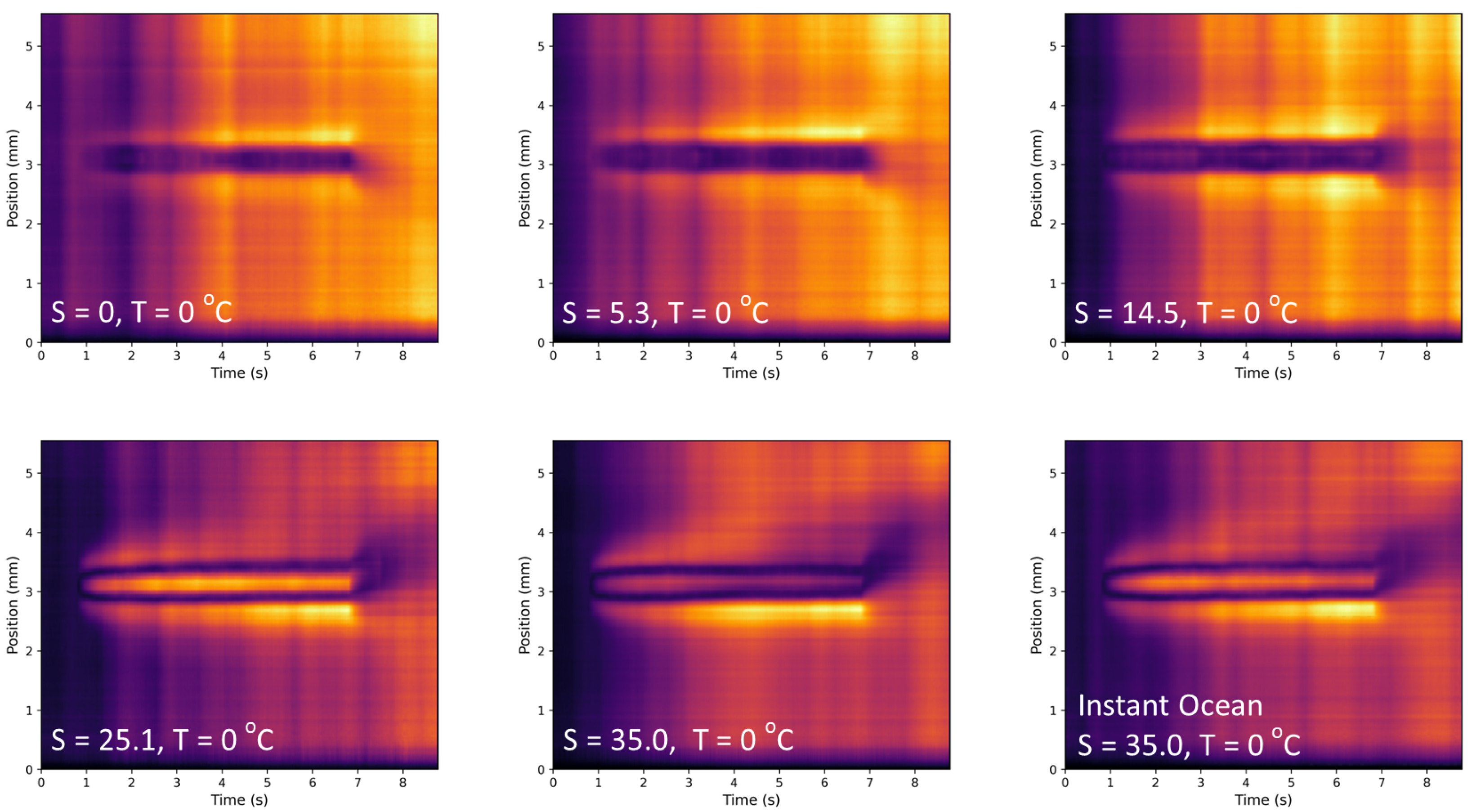
In the analysis of the heatmaps for a temperature of 0 °C across the range of salinities investigated, one sees the expected behavior of the thermal starting plumes. Specifically, one sees both a descending thermal ending plume for pure water and and a fully frustrated thermal ending plume for . Ascending thermal ending plumes are seen for , , and Instant Ocean®. Moreover, asymmetry in integration region 1 changes from stronger above the laser region to stronger below it with increasing salinity. These observations are presented in Figure 13.
For salinities below 23, the temperature of maximum density surpasses the melting point. This characteristic gives rise to a unique behavior in the thermal plumes [14]. Specifically, when salinity is set at 0 and 5, descending frustrated thermal starting plumes become evident. Figure 11 shows that, for , fully frustrated thermal starting plumes occur at °C, and for , they occur at °C. Conversely, the scenario changes for a salinity level of 14.5, where the system exhibits a fully frustrated thermal starting plume. These values suggest laser-induced heating of for and for .
In contrast, for salinities of 25.1 and 35.0 and Instant Ocean® (), ascending frustrated thermal starting plumes dominate the observed behavior. Under these conditions, all thermal starting plumes are less dense than the ambient fluid.
5. Conclusions
The findings presented in this study provide insight into the nature of thermal plume dynamics, particularly for pure and saltwater systems near their respective temperatures of maximum density. Analysis employing the photothermal imaging technique has revealed critical insights into the behavior of frustrated thermal starting plumes. These plumes, characterized by their almost equivalent buoyant and weight forces near the temperature of maximum density, exhibit unique patterns of movement, ranging from stagnation to descending motion, a stark contrast to the typical ascending thermal plumes seen in all other common liquids.
In pure water, the occurrence of maximum density at approximately 4 °C plays a unique role in thermal starting plume dynamics compared to other molecular liquids. This study has demonstrated that the transition from ascending to descending convection, as seen at about 2.3 °C, exemplifies the more complex interplay of temperature, density, and buoyancy in pure water compared to other molecular liquids. The saltwater scenarios add another layer of complexity. The presence of Na+ and Cl− ions disrupts the hydrogen bonding among water molecules, leading to a shift in the temperature of maximum density. For low salinities, there remains a significant-enough gap between the melting point and the temperature of maximum density. Ascending, descending, and fully frustrated thermal starting plumes were observed. For higher values of salinity, only ascending thermal starting plumes can occur. This understanding has potential implications for the study of natural and human-made thermal plumes in various water bodies.
In the future, investigators could (i) consider more extreme temperature and pressure situations, (ii) study the effect of dissolved organic matter, in particular relatively stronger absorbers such as alcohols and amines, (iii) study plumes in nonhomogeneous fluids such as layered salt solutions, (iv) develop protocols such as producing a thermal followed by a thermal starting plume [60], and (v) employ computational fluid dynamics simulations.
Author Contributions
Conceptualization, D.J.U.; methodology, D.J.U.; software, D.J.U.; validation, D.J.U., J.B., K.S., J.D.L. and M.W.G.; formal analysis, D.J.U., J.B., K.S., J.D.L. and M.W.G.; investigation, D.J.U., J.B., K.S. and J.D.L.; resources, D.J.U. and K.S.; data curation, D.J.U., K.S. and M.W.G.; writing—original draft preparation, D.J.U.; writing—review and editing, D.J.U., J.B., K.S., J.D.L. and M.W.G.; visualization, D.J.U., J.B,. K.S., J.D.L. and M.W.G.; supervision, D.J.U. and K.S.; project administration, D.J.U.; funding acquisition, D.J.U. and K.S. All authors have read and agreed to the published version of the manuscript.
Funding
This research received no external funding.
Data Availability Statement
The raw and processed data sets are available at www.darinulness.com/research/data/frustrated (accessed on 14 December 2023). The code for the data-acquisition program and data analysis programs can be found at https://github.com/ulnessd/ThermalLensing/ (accessed on 14 December 2023).
Acknowledgments
The authors acknowledge Jahan Dawlaty and Daniel Turner for valuable discussions. Internal funding for this work was provided by the Office of Undergraduate Research, Scholarship, and Creative Activity (URSCA) at Concordia College, the Concordia College Strategic Initiative Fund, and the Chemistry Department Endowed Research Fund.
Conflicts of Interest
The authors declare no conflicts of interest. The funders had no role in the design of the study; in the collection, analyses, or interpretation of the data; in the writing of the manuscript; nor in the decision to publish the results.
References
- Dominguez Lopez, J.; Gealy, M.W.; Ulness, D.J. Photothermal Imaging of Transient and Steady State Convection Dynamics in Primary Alkanes. Liquids 2023, 3, 371–384. [Google Scholar] [CrossRef]
- Franko, M.; Tran, C.D. Water as a Unique Medium for Thermal Lens Measurements. Anal. Chem. 1989, 61, 1660–1666. [Google Scholar] [CrossRef]
- Franko, M.; Tran, C.D. Thermal Lens Effect in Electrolyte and Surfactant Media. J. Phys. Chem. 1991, 95, 6688–6696. [Google Scholar] [CrossRef]
- Turner, J.S. Buoyancy Effects in Fluids; Cambridge University Press: Cambridge, UK, 1973. [Google Scholar]
- Raven, P.H.; Johnson, G.B.; Mason, K.A.; Losos, J.B.; Singer, S.R. Biology, 9th ed.; McGraw-Hill: New York, NY, USA, 2011. [Google Scholar]
- Speer, K.G.; Rothery, D.A. Thermocline Penetration by Buoyant Plumes. Philos. Trans. Math. Phys. Eng. Sci. 1997, 355, 443–458. [Google Scholar] [CrossRef]
- Thomson, R.E.; Delaney, J.R. Evidence for a Weakly Stratified Europan Ocean Sustained by Seafloor Heat Flux. J. Geophys. Res. 2001, 106, 12355–12365. [Google Scholar] [CrossRef]
- Di Iorio, D.; Lavelle, J.W.; Rona, P.; Bemis, K.; Xu, G.; Germanovich, L.; Lowell, R.; Genc, G. Measurements and Models of Heat Flux and Plumes from Hydrothermal Discharges Near the Deep Seafloor. Oceanography 2012, 25, 168–179. [Google Scholar] [CrossRef]
- Faulkner, A.; Bulgin, C.E.; Merchant, C.J. Coastal Tidal Effects on Industrial Thermal Plumes in Satellite Imagery. Remote Sens. 2019, 11, 2132. [Google Scholar] [CrossRef]
- Faulkner, A.; Bulgin, C.E.; Merchant, C.J. Characterizing Industrial Thermal Plumes in Coastal Regions Using 3-D Numerical Simulations. Environ. Res. Commun. 2021, 3, 045003. [Google Scholar] [CrossRef]
- Wei, J.; Feng, L.; Tong, Y.; Xu, Y.; Shi, K. Long-Term Observation of Global Nuclear Power Plants Thermal Plumes Using Landsat Images and Deep Learning. Remote Sens. Environ. 2023, 295, 113707. [Google Scholar] [CrossRef]
- Woods, A.W. Turbulent Plumes in Nature. Annu. Rev. Fluid Mech. 2010, 42, 391–412. [Google Scholar] [CrossRef]
- Stanley, S.M. Earth System History, 2nd ed.; W.H. Freeman: New York, NY, USA, 2005. [Google Scholar]
- Wiesenburg, D.A.; Little, B.J. A Synopsis of the Chemical/Physical Properties of Seawater. Ocean Phys. Eng. 1987, 12, 127–165. [Google Scholar]
- Grace, A. Numerical Simulations of Convection and Gravity Currents near the Temperature of Maximum Density. Ph.D. Thesis, University of Waterloo, Waterloo, ON, Canada, 2022. [Google Scholar]
- Morton, B.R.; Taylor, G.; Turner, J.S. Turbulent Gravitational Convection from Maintained and Instantaneous Sources. Proc. R. Soc. Lond. Ser. A Math. Phys. Sci. 1956, 234, 1–23. [Google Scholar]
- Turner, J.S. The ‘Starting Plume’ in Neutral Surroundings. J. Fluid Mech. 1962, 13, 356–368. [Google Scholar] [CrossRef]
- Whinnery, J.R.; Miller, D.T.; Dabby, F. Thermal Convection and Spherical Aberration Distortion of Laser Beams in Low-Loss Liquids. IEEE Quantum Electron. 1967, 3, 382–383. [Google Scholar] [CrossRef]
- Hunt, G.R.; Van Den Bremer, T.S. Classical Plume Theory: 1937–2010 and Beyond. IMA J. Appl. Math. 2011, 76, 424–448. [Google Scholar] [CrossRef]
- Moses, E.; Zocchi, G.; Procaccia, I.; Libchaber, A. The Dynamics and Interaction of Laminar Thermal Plumes. Europhys. Lett. 1991, 14, 55–60. [Google Scholar] [CrossRef]
- Davaille, A.; Limare, A.; Touitou, F.; Kumagai, I.; Vatteville, J. Anatomy of a Laminar Starting Thermal Plume at High Prandtl Number. Exp. Fluids 2011, 50, 285–300. [Google Scholar] [CrossRef]
- Kundu, P.K.; Cohen, I.M. Fluid Mechanics, 3rd ed.; Elsevier: Amsterdam, The Netherlands, 2004. [Google Scholar]
- Richards, M.K.; Coker, O.E.; Florido, J.; Nicholls, R.A.M.; Ross, A.N.; Rooney, G.G. On the Near-Field Interaction of Vertically Offset Turbulent Plumes. J. Fluid Mech. 2023, 966, A24. [Google Scholar] [CrossRef]
- Zhao, W.; Chen, S.; Yang, J.; Zhou, W. Assessment of RANS Turbulence Models in Prediction of the Hydrothermal Plume in the Longqi Hydrothermal Field. Appl. Sci. 2023, 13, 7496. [Google Scholar] [CrossRef]
- Wang, K.; Han, X.; Wang, Y.; Cai, Y.; Qiu, Z.; Zheng, X. Numerical Simulation-Based Analysis of Seafloor Hydrothermal Plumes: A Case Study of the Wocan-1 Hydrothermal Field, Carlsberg Ridge, Northwest Indian Ocean. J. Mar. Sci. Eng. 2023, 11, 1070. [Google Scholar] [CrossRef]
- Papanicolaou, P.N. Entrainment in Buoyant Jets and Fountains Revisited. Environ. Fluid Mech. 2023, 1–24. [Google Scholar] [CrossRef]
- Wise, N.H.; Hunt, G.R. General Solutions of the Plume Equations: Towards Synthetic Plumes and Fountains. J. Fluid Mech. 2023, 973, R2. [Google Scholar] [CrossRef]
- Bialkowski, S.E.; Astrath, N.G.C.; Proskurnin, M.A. Photothermal Spectroscopy Methods, 2nd ed.; Wiley: Hoboken, NJ, USA, 2019. [Google Scholar]
- Liu, M.; Franko, M. Thermal Lens Spectrometry: Still a Technique on the Horizon? Int. J. Thermophys. 2016, 37, 67. [Google Scholar] [CrossRef]
- Bertolotti, M.; Li Voti, R. A Note on the History of Photoacoustic, Thermal Lensing, and Photothermal Deflection Techniques. J. Appl. Phys. 2020, 128, 230901. [Google Scholar] [CrossRef]
- Proskurnin, M.A.; Khabibullin, V.R.; Usoltseva, L.O.; Vyrko, E.A.; Mikheev, I.V.; Volkov, D.S. Photothermal and optoacoustic spectroscopy: State of the art and prospects. Phys. Uspekhi 2022, 65, 270–312. [Google Scholar] [CrossRef]
- Fang, H.L.; Swofford, R.L. The Thermal Lens in Absorption Spectroscopy. In Ultrasensitive Laser Spectroscopy; Kliger, D.S., Ed.; Academic Press: New York, NY, USA, 1983. [Google Scholar]
- Gordon, J.P.; Leite, R.C.C.; Moore, R.S.; Porto, S.P.S.; Whinnery, J.R. Long-Transient Effects in Lasers with Inserted Liquid Samples. J. Appl. Phys. 1965, 36, 3–8. [Google Scholar] [CrossRef]
- Carman, R.I.; Kelley, P.I. Time dependence in the thermal blooming of laser beams. Appl Phys. Lett. 1968, 12, 241–243. [Google Scholar] [CrossRef]
- O’Neil, R.W.; Kleiman, H.; Lowder, J.E. Observation of hydrodynamic effects on thermal blooming. Appl. Phys. Lett. 1972, 24, 118–120. [Google Scholar] [CrossRef]
- Hayes, J.N. Thermal Blooming of Laser Beams in Fluids. Appl. Opt. 1972, 11, 455–461. [Google Scholar] [CrossRef]
- Long, M.E.; Swofford, R.L.; Albrecht, A.C. Thermal Lens Technique: A New Method of Absorption Spectroscopy. Science 1976, 191, 183–185. [Google Scholar] [CrossRef]
- Boccara, A.C.; Fournier, D.; Jackson, W.; Amer, N.S. Sensitive photothermal deflection technique for measuring absorption in optically thin media. Opt. Lett. 1980, 5, 377–379. [Google Scholar] [CrossRef] [PubMed]
- Jackson, W.B.; Amer, N.M.; Boccara, A.C.; Fournier, D. Photothermal deflection spectroscopy and detection. Appl. Opt. 1981, 20, 1333–1344. [Google Scholar] [CrossRef]
- Longaker, P.R.; Litvak, M.M. Perturbation of the refractive index of absorbing media by a pulsed laser beam. J. Appl. Phys. 1969, 40, 4033–4041. [Google Scholar] [CrossRef]
- Lee, D.; Albrecht, A.C. On global energy conservation in nonlinear light—Matter interaction: The nonlinear spectroscopies, active and passive. In Advances in Chemical Physics; Prigogine, I., Rice, S.A., Eds.; John Wiley & Sons: Hoboken, NJ, USA, 1993; Volume 83, pp. 43–87. [Google Scholar]
- Singhal, S.; Goswami, D. Thermal Lens Study of NIR Femtosecond Laser-Induced Convection in Alcohols. ACS Omega 2019, 4, 1889–1896. [Google Scholar] [CrossRef]
- Kumar Rawat, A.; Chakraborty, S.; Kumar Mishra, A.; Goswami, D. Achieving Molecular Distinction in Alcohols with Femtosecond Thermal Lens Spectroscopy. Chem. Phys. 2022, 561, 111596. [Google Scholar] [CrossRef]
- Goswami, D. Intense Femtosecond Optical Pulse Shaping Approaches to Spatiotemporal Control. Front. Chem. 2023, 10, 1006637. [Google Scholar] [CrossRef]
- Rawat, A.K.; Chakraborty, S.; Mishra, A.K.; Goswami, D. Unraveling Molecular Interactions in Binary Liquid Mixtures with Time-Resolved Thermal-Lens-Spectroscopy. J. Mol. Liq. 2021, 336, 116322. [Google Scholar] [CrossRef]
- Singhal, S.; Goswami, D. Unraveling the Molecular Dependence of Femtosecond Laser-Induced Thermal Lens Spectroscopy in Fluids. Analyst 2020, 145, 929–938. [Google Scholar] [CrossRef]
- Khabibullin, V.R.; Usoltseva, L.O.; Galkina, P.A.; Galimova, V.R.; Volkov, D.S.; Mikheev, I.V.; Proskurnin, M.A. Measurement Precision and Thermal and Absorption Properties of Nanostructures in Aqueous Solutions by Transient and Steady-State Thermal-Lens Spectrometry. Physchem 2023, 3, 156–197. [Google Scholar] [CrossRef]
- Wang, Z.; Li, S.; Chen, R.; Zhu, X.; Liao, Q. Simulation on the Dynamic Flow and Heat and Mass Transfer of a Liquid Column Induced by the IR Laser Photothermal Effect Actuated Evaporation in a Microchannel. Int. J. Heat Mass Transf. 2017, 113, 975–983. [Google Scholar] [CrossRef]
- Buffett, C.E.; Morris, M.D. Convective Effects in Thermal Lens Spectroscopy. Appl. Spectrosc. 1983, 37, 455–458. [Google Scholar] [CrossRef]
- Fang, H.L.; Swofford, R.L. Highly Excited Vibrational States of Molecules by Thermal Lensing Spectroscopy and the Local Mode Model. II. Normal, Branched, and Cycloalkanes. J. Phys. Chem. 1980, 73, 2607–2617. [Google Scholar] [CrossRef]
- Fang, H.L.; Meister, D.M.; Swofford, R.L. Overtone Spectroscopy of Nonequivalent Methyl C-H Oscillators. Influence of Conformation on Vibrational Overtone Energies. J. Phys. Chem. 1984, 88, 410–416. [Google Scholar] [CrossRef]
- Tran, C.D.; Grishko, V.I.; Baptista, M.S. Nondestructive and Nonintrusive Determination of Chemical and Isotopic Purity of Solvents by Near-Infrared Thermal Lens Spectrometry. Appl. Spectrosc. 1994, 48, 833–842. [Google Scholar] [CrossRef]
- Holder, E.L.; Conmy, R.N.; Venosa, A.D. Comparative Laboratory-Scale Testing of Dispersant Effectiveness of 23 Crude Oils Using Four Different Testing Protocols. J. Environ. Prot. 2015, 6, 628–639. [Google Scholar] [CrossRef]
- ChatGPT 4.0. Available online: http://openai.com (accessed on 15 May 2023).
- Péron, J.-J.; Bourdéron, C.; Sandorfy, C. On the Existence of Free OH Groups in Liquid Water. Can. J. Chem. 1971, 49, 3901–3903. [Google Scholar] [CrossRef]
- Cornish-Bowden, A. Fundamentals of Enzyme Kinetics; Butterworths: Boston, MA, USA, 1979. [Google Scholar]
- Magazu, S.; Maisano, G.; Majolino, D.; Mallamace, F.; Migliardo, P.; Aliotta, F.; Vasi, C. Relaxation process in deeply supercooled water by Mandelstam-Brillouin scattering. J. Phys. Chem. 1989, 93, 942–947. [Google Scholar] [CrossRef]
- Magazu, S.; Maisano, G.; Mallamace, F.; Micali, N. Growth of fractal aggregates in water solutions of macromolecules by light scattering. Phys. Rev. A 1989, 39, 4195. [Google Scholar] [CrossRef] [PubMed]
- Crupi, V.; Jannelli, M.P.; Magazu, S.; Maisano, G.; Majolino, D.; Migliardo, P.; Sirna, D. Rayleigh wing and Fourier transform infrared studies of intermolecular and intramolecular hydrogen bonds in liquid ethylene glycol. Mol. Phys. 1995, 84, 645–652. [Google Scholar] [CrossRef]
- Wang, N.; Xu, Y.; Zhang, W.; Zhou, X. Study on the Development of a Laminar Buoyant Starting Plume Following a Thermal. Int. J. Therm. Sci. 2023, 192, 108442. [Google Scholar] [CrossRef]
Figure 1.
Caricatures of the thermal buoyancy effects following Turner’s definitions [4]. Thermal starting plumes (a) represent transient states consisting of a rising plumehead connected to a constant heat source via a conduit (see Figure 2). This process ultimately reaches the steady-state form of the thermal plume (b). Under conditions near the temperature of maximum density, the buoyant force is very small and positive, indicating an ascending frustrated thermal plume, or zero, indicating a fully frustrated thermal starting plume (c), or very small and negative, indicating a descending frustrated thermal starting plume (d). Arrows indicate direction of fluid flow.

Figure 2.
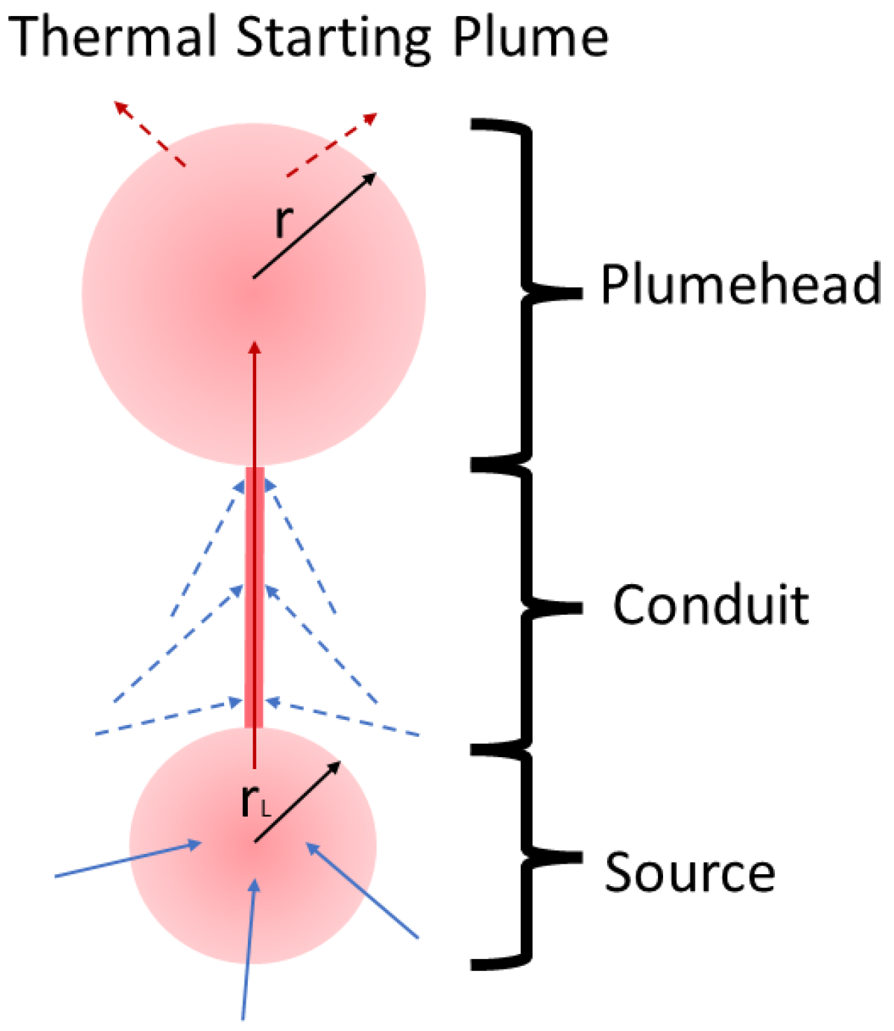
Key features of a typical thermal starting plume. The anatomy of a thermal starting plume consists of a heat source (in this study, the IR excitation laser), a plumehead, and a conduit. Mass is entrained through the conduit as indicated by the blue dashed arrows. Additionally, it is suggested here that mass is also entrained by entering the laser-heated region, as shown by the solid blue arrows. The dashed red arrows represent heat loss across the sharp temperature boundary of the plumehead. Upon heating with the IR laser, a plumehead begins to form and, due to its lower density resulting from laser heating, starts to ascend. This ascent draws in mass through entrainment, causing the plumehead to expand as it rises. The is the radius of the laser beam and r is the radius of the plumehead.
Figure 2.
Key features of a typical thermal starting plume. The anatomy of a thermal starting plume consists of a heat source (in this study, the IR excitation laser), a plumehead, and a conduit. Mass is entrained through the conduit as indicated by the blue dashed arrows. Additionally, it is suggested here that mass is also entrained by entering the laser-heated region, as shown by the solid blue arrows. The dashed red arrows represent heat loss across the sharp temperature boundary of the plumehead. Upon heating with the IR laser, a plumehead begins to form and, due to its lower density resulting from laser heating, starts to ascend. This ascent draws in mass through entrainment, causing the plumehead to expand as it rises. The is the radius of the laser beam and r is the radius of the plumehead.

Figure 3.
Schematic of the experimental setup. The excitation beam is from a QSL103A—1030 nm Q-Switched Picosecond Microchip Laser System (Thorlabs). The probe laser is from a 5 V 650 nm laser diode (HiLetgo, Huanqiu Wuliu Zhongxin, HuaNanCheng, PingHu, LongGang, Shenzhen, Guangdong, China). The shutter is driven by a solenoid controlled by the computer (Raspberry Pi 4, Pencoed, Wales). The Arducam Camera (Kowloon, Hong Kong) is equipped with a 5-megapixel Omnivision (Santa Clara, CA, USA) OV5647 sensor and controlled by the computer. The heater/chiller is an FTS (Howell, MI, USA) model RS33AL10 running ethylene glycol and offering a ±0.5 °C stability over the course of the data acquisition.

Figure 4.
Still frames from the raw (top row) and background-subtracted (bottom row) data video files for a 20-run average of pure water at 70 °C. The left column is approximately 2.16 s into the run, or 0.16 s after the laser first enters the sample. The middle column is approximately 2.47 s into the run (0.47 s after the laser). The right column is approximately 3.19 s into the run (1.19 s after the laser).

Figure 5.
Example of a heatmap representation of the video data shown in Figure 4. The heatmap for pure water at 70 °C shows a visually pronounced rising plumehead and source. Reading from left-to-right across the heatmap, one would first see in the raw video file (Figure 4) the constant background. At about 0.8 s, evidence of the thermal lens would appear at the position of the laser. Progressing further to the right on the heatmap would correspond to seeing the plumehead start to rise. Between 3 and 4 s, the plumehead would be exiting the frame. The conduit is barely visible because the temperature gradient is not as abrupt as for the leading edge of the plumehead and the laser heating region. The laser lies along the horizontal green line and appears as a visually pronounced horizontal streak. It is this green line over which the kinetics traces will be taken in subsequent analysis. The pronounced feature below this is the effect of the thermal lens bending light to the outside of the cylinder. The vertical green line indicates the point of plumehead formation. When the shutter closes, the heated fluid in the laser region quickly rises in a thermal ending plume. The ascension angle, , is marked with an angled green line. The curly brackets indicate the integration regions (referred to as region 1 and region 2) over which the signal is averaged. region 1 is used to obtain a more quantitative representation of the steady-state regime. region 2 is used to capture the behavior of the thermal ending plume.

Figure 6.
Heatmaps for pure water for temperatures 11 °C to 70 °C. The features of the heatmaps as depicted in Figure 5 are evident. A shortening of the time to form the plumehead and a quickening of the rise of the plumehead with increasing temperature is evident. While it is visually clear that the signal-to-noise ratio is decreasing with temperature, all signals are clearly evident above the background.

Figure 7.
Heatmaps for pure water for temperatures 0 °C to 10 °C. At these temperatures, the signal-to-noise ratio is becoming poor. A rising plumehead is evident down to at least 7 °C. The ascension angle of the thermal ending plume is rapidly decreasing, in contrast to what is evident in Figure 6, where it remains nearly constant. Ascension angles are plotted in Figure 9. Indirect evidence of transition from ascending to descending frustrated thermal starting plumes is seen by assessing the relative strengths of the light accumulation above and below the laser position.

Figure 8.
Lensing-corrected total integrated signal, , for pure water (solid circles) and Instant Ocean® (solid inverted triangles). Because the high salt concentration reduces the effectiveness of hydrogen bonding, the Instant Ocean® data follow a curve that is less steep than that for water. Both sets of data are fit to Equation (3). Data points in black were not included in their respective fits (blue for water and green for Instant Ocean®). The fit parameters for water are , °C, °C, and . The fit parameters for Instant Ocean® are , °C, °C, and . The curves cross at 30.4 °C. Because the lens-corrected total integrated signal is determined from the averaged data set, individual error bars are not generated. However, it is estimated that, for the fit data (blue and green points), the relative standard deviation is approximately 2.25%.

Figure 9.
Ascension angles, , for thermal ending plumes in pure water. The data appear to follow a function of the form . Fit parameters are °C, °C−1, and °C.
Figure 9.
Ascension angles, , for thermal ending plumes in pure water. The data appear to follow a function of the form . Fit parameters are °C, °C−1, and °C.

Figure 10.
Spatial profiles for integration region 1 (left curly brackets shown in Figure 5). Here, the spatial position is shifted to center on the position of the laser. The graph compares temperatures 0 °C through 5 °C. Visual inspection of the asymmetry of the left and right peaks suggests the fully frustrated thermal starting plume occurs between 2 °C and 3 °C.

Figure 11.
(top row) Characterization of the thermal ending plumes for the cases of °C through °C for pure water (left panel), salinity S = 5.3 (middle panel), and salinity S = 14.5 (right panel). For the water case, the temperature increases by 1 °C through the bottom-to-top progression of the graphs (blue corresponding to and red corresponding to ). For the salt waters cases, the temperature increases by 2 °C (same color scheme). These curves are the results for the figure integrated region 2 in Figure 5. A vertical offset was added to each curve for visual clarity. Further, the abscissa is zeroed at the point of the laser (green horizontal line in Figure 5). The troughs were fit to a quadratic function for a small range near their minima. (bottom row) The minima of the fit curves are plotted versus temperature (fit parameters: water mm−1 and ; salinity , mm−1 and ; salinity , mm−1 and ). The x intercepts of the fit lines give the temperature of the fully frustrated thermal starting plume. These are °C (water), °C (salinity ), and °C (salinity ).

Figure 12.
Kinetics traces for pure water. The time behavior along the horizontal green line in Figure 5 is shown in the panel on the left. The various temperature graphs are given independent vertical offset for visual clarity. A diminishing and delaying of the time to form the plumehead (vertical green line in Figure 5) upon cooling are evident. The plot on the right shows the time to form the plumehead, , (from the peaks of the kinetics traces) versus temperature for water (blue) and Instant Ocean® (green; kinetics traces not shown). The data are fit to . The fit parameters are s·°C, °C, and s for water and s·°C, °C, and s for Instant Ocean®.

Figure 13.
Heatmaps for °C for the various salinities used in this study. For , the temperature of maximum density is greater than the melting point. Descending frustrated thermal starting plumes are seen for and . The case of exhibits a fully frustrated thermal starting plume. Finally, ascending frustrated thermal starting plumes are seen for , , and Instant Ocean® prepared to .

Disclaimer/Publisher’s Note: The statements, opinions and data contained in all publications are solely those of the individual author(s) and contributor(s) and not of MDPI and/or the editor(s). MDPI and/or the editor(s) disclaim responsibility for any injury to people or property resulting from any ideas, methods, instructions or products referred to in the content. |
© 2024 by the authors. Licensee MDPI, Basel, Switzerland. This article is an open access article distributed under the terms and conditions of the Creative Commons Attribution (CC BY) license (https://creativecommons.org/licenses/by/4.0/).
Share and Cite
MDPI and ACS Style
Biebighauser, J.; Dominguez Lopez, J.; Strand, K.; Gealy, M.W.; Ulness, D.J. Frustrated-Laser-Induced Thermal Starting Plumes in Fresh and Salt Water. Liquids 2024, 4, 332-351. https://doi.org/10.3390/liquids4020017
AMA Style
Biebighauser J, Dominguez Lopez J, Strand K, Gealy MW, Ulness DJ. Frustrated-Laser-Induced Thermal Starting Plumes in Fresh and Salt Water. Liquids. 2024; 4(2):332-351. https://doi.org/10.3390/liquids4020017
Chicago/Turabian StyleBiebighauser, Johnathan, Johan Dominguez Lopez, Krys Strand, Mark W. Gealy, and Darin J. Ulness. 2024. "Frustrated-Laser-Induced Thermal Starting Plumes in Fresh and Salt Water" Liquids 4, no. 2: 332-351. https://doi.org/10.3390/liquids4020017