Real-Time Optimization of Social Distancing to Mitigate COVID-19 Pandemic Using Quantized Extremum Seeking

Abstract

The application of extremum seeking control is investigated to mitigate the spread of the COVID-19 pandemic, maximizing social distancing while limiting the number of infections. The procedure does not rely on the accurate knowledge of an epidemiological model and takes realistic constraints into account, such as hospital capacities, the observation horizon of the pandemic evolution and the quantized government sanitary policy decisions. Based on the bifurcation analysis of a SEIARD compartmental model providing two possible types of equilibria, numerical simulation reveals the transient behaviour of the extremum of the constrained cost function, which, if rapidly caught by the algorithm, slowly drifts to the steady-state optimum. Specific features are easily incorporated in the real-time optimization procedure, such as quantized sanitary condition levels and long actuation (decision) periods (usually several weeks), requiring processing of the discrete control signal saturation and quantization. The performance of the proposed method is numerically assessed, considering the convergence rate and accuracy (quantization bias).

1. Introduction

Since January 2020, human society has been deeply impacted by the COVID-19 pandemic. In this context, mathematical modeling and numerical simulation of the virus spread as a function of several factors, including social distancing, testing and quarantining, mobility restrictions and vaccination, have been playing a key role in the decision policy of many governments worldwide [1]. The most popular dynamic model finds its origin in the work of [2], who proposed a compartmental representation, categorizing people in several possible states such as susceptible (S), symptomatic Infected (I) or Removed/Recovered (R). The so-called SIR models provide predictions based on historical data and can be used to develop hypothetical control strategies. For instance, Ref. [3] proposes an optimal SEIAR model-based open-loop control approach (adding the Exposed and Asymptomatic compartments) and suggests that on-off policies alternating between strict social distancing and relaxing can be effective at flattening the infection curve. Furthermore, Ref. [4] investigates open-loop optimal control as well as model predictive control (MPC) with online adaptation of the social policy constraint, and robust MPC using interval state estimation to take account of uncertainties in the model and measurements. In the same spirit, Ref. [5] develops an MPC control strategy taking account of time-dependent specifications and logical relations between model variables, and multiple predefined discrete levels of governmental interventions (control input quantization). As all the model variables are not accessible to measurements, it is necessary to develop state estimators in order to apply full-state feedback, which poses additional challenges. In [4], an interval observer is developed, whereas an observer for Linear Parameter Varying (LPV) systems is designed in [5].

Data-driven control methods have also attracted interest, with different optimal formulations, such as in [6], showing that the cost of eradicating the disease may be significantly higher than the cost of managing the pandemic by hospital saturation limitations, which is claimed to be the policy adopted by several US local administrations. Ref. [7] also recommend deep-learning-based strategies to mitigate the pandemic, assimilating a high number of data samples to approach hyper parameters (effective reproduction number of the virus over time, hospitalization rate, etc).

As stressed in [8], one can of course question the validity of the dynamic prediction models, and several recent research papers have proposed real-time optimization (RTO) strategies to take model uncertainties into account either by considering robust-to-mismatch or, more radically, model-free techniques. In one of our recent publications [9], discrete model-free extremum seeking (ES) has been been applied for the first time to the control of social distancing while avoiding hospital saturation. This contrasts with the first MPC-based studies of [3,4], which only aim at limiting the infectious cases in a conservative way.

Another emerging research stream aims at assessing the risk of several alternative control policies including the consideration of vaccination strategies guided by socio-demographic and health factors [10] as well as the possible withdrawal of the vaccination passport to grant more freedom [11].

In this connection, more elaborate objective/cost functions are considered, such as [12], who proposes a concomitant optimization objective with the concern of providing advanced solutions considering people psychological health. In the same stream of studies, Ref. [13] develops an original sliding-mode-based RTO design, adapted to a SIRDQ model with the objective of reducing the quarantine period while guaranteeing an effective regulation of the reproduction number to a desired value. Several numerical validations are proposed using first-order sliding-mode and second-order super-twisting methods.

The objective of the present study is to investigate the application of model-free quantized discrete extremum seeking control (QESC) to achieve the optimization of social distancing while mitigating the pandemic and limiting the number of infection cases. Extremum seeking control (ESC) is an RTO method achieving a direct input adaptation [14] to reach a steady-state map extremum, either by tracking an uncertain model-based trajectory [15] or by relying on the existence of a measurable convex objective function without any a priori knowledge about the process model [16]. The latter is also denominated as model-free perturbation-based ES and aims at estimating the objective function gradient and forcing its estimate to zero while persistently exciting the input using a periodic dither signal. Several review papers highlight the potential of the ES methods to solve RTO problems in different scientific fields (see, for instance, [17,18], for reviews of ESC developments over the last few decades).

As underlined in [9], discrete ESC presents some operating challenges such as the condition of persistency of excitation [19], which prevents the output signal from reaching a true steady-state (the latter is only achieved on average [16]), the convergence dependency on the dither signal frequency which should be adapted to the process operating conditions and time constants [20], and the nature of the actuator, which is not assumed to present saturation or quantized levels. The latter issue has recently been tackled by [21], based on the work of [22], who lay the foundations of the anti-windup ESC providing stability and convergence proofs. However, actuator saturation and quantization studies in the framework of ESC are limited to two-level situations and, in this work, an extension to multiple quantized levels is proposed, which corresponds to the various social distancing levels that could be imposed in a governmental policy.

The motivation of this work is therefore to extend our preliminary results [9] in order to include a rigorous treatment of saturation and quantization of the control signal (i.e., social distancing in the context of the pandemic) using the results of [21]. To sum up, the objectives are to design (i) a procedure focusing on psychological health and the reduction of social distancing since hospitals should be less and less likely to overpass their bed capacities thanks to the vaccination, (ii) a realistic discrete software tool supporting decision policies without requiring significant computational loads (in contrast with, for instance, deep-learning based methods) and (iii) the first validation of a QESC strategy in the framework of the COVID-19 pandemic.

The next section presents the epidemiological model used in [3] as an emulator of the population behavior to test the ESC approaches. Section 2.2 computes the equilibrium points of the model and demonstrates a bifurcation behavior depending on the level of social distancing. In Section 2.3, a measurable cost function is proposed, which will use the concept of barrier functions, and serves as basis for ESC, which is further discussed in Section 3. The numerical application is detailed in Section 4, where the two time scales of the convergence are highlighted and the issue of quantization of the measures is introduced. The final section is dedicated to conclusions and research perspectives.

2. COVID-19 Outbreak Modeling

2.1. SIR Modeling

Compartmental population modeling [2] is, by far, the most common formalism to model epidemics and describe the transitions between susceptible $S\left(t\right)$, infected $I\left(t\right)$ and removed/recovered $R\left(t\right)$ states. In [9], the compartmental SEAIR model of [3] describing the COVID-19 outbreak is considered, which also accounts for the asymptomatic population $A\left(t\right)$ (this class of individuals gathers cases which are not detected due to asymptomatic conditions, or due to the lack of testing) as well as the exposed population $E\left(t\right)$. This model also includes mortality, with a perished population $P\left(t\right)$, but no natality. The resulting dynamics of the several compartmental variables are represented by an ordinary differential equation system as follows:

$$\begin{array}{cc}\hfill \frac{dS}{dt}& =\frac{-{\alpha }_a\left(t\right)S\left(t\right)A\left(t\right)-{\alpha }_i\left(t\right)S\left(t\right)I\left(t\right)}{N}+\gamma R\left(t\right),\hfill \end{array}$$

(1a)

$$\begin{array}{cc}\hfill \frac{dE}{dt}& =\frac{{\alpha }_a\left(t\right)S\left(t\right)A\left(t\right)+{\alpha }_i\left(t\right)S\left(t\right)I\left(t\right)}{N}-lE\left(t\right),\hfill \end{array}$$

(1b)

$$\begin{array}{cc}\hfill \frac{dA}{dt}& =lE\left(t\right)-\kappa \left(t\right)A\left(t\right)-\rho A\left(t\right),\hfill \end{array}$$

(1c)

$$\begin{array}{cc}\hfill \frac{dI}{dt}& =\kappa \left(t\right)A\left(t\right)-\beta I\left(t\right)-\mu I\left(t\right),\hfill \end{array}$$

(1d)

$$\begin{array}{cc}\hfill \frac{dR}{dt}& =\rho A\left(t\right)+\beta I\left(t\right)-\gamma R\left(t\right),\hfill \end{array}$$

(1e)

$$\begin{array}{cc}\hfill \frac{dP}{dt}& =\mu I\left(t\right),\hfill \end{array}$$

(1f)

where N is the total population and S, E, A, I, R, and P are, respectively, the susceptible, exposed, unreported infected (asymptomatic or unconfirmed), reported/confirmed infected, removed/recovered and perished populations. The parameters ${\alpha }_a$ and ${\alpha }_i$ are the rates of exposure to the A and I populations, respectively. ${\alpha }_a$ characterizes, in a broad sense, social distancing and ${\alpha }_i$, quarantining, and can be considered as manipulated (control) inputs from a system and control perspective, as well as the screening/testing rate $\kappa$. Constant (at least in first approximation) parameters account for the (inverse of the) latent period of the virus l ($0.5$days${}^{-1}$), the infectious period of unconfirmed cases $\rho$ ($0.1$days${}^{-1}$) and the recovery rate $\beta$ ($0.025$days${}^{-1}$). These parameters represent the situation in the US in 2020 according to [3].

2.2. Bifurcation Analysis

Neglecting the death rate $\mu$, which is fortunately very low as compared to the recovery rate $\gamma$ (one to two orders of magnitude smaller) and considering a constant total population N in model (1), two equilibrium points can be obtained, which correspond either to the extinction of the infection (the steady-state susceptible population level is $S_{ss}=N$ and all other variables are 0) or to the stabilization of the epidemics, i.e., non-zero steady-state values of the several variables depending on the several rates defined in

Table 1. Parameter values in model (1).

N	${\mathit{\alpha }}_{\mathit{i}}$$\left[{\mathit{d}}^{-1}\right]$	$\mathit{\kappa }$$\left[{\mathit{d}}^{-1}\right]$	$\mathit{\beta }$$\left[{\mathit{d}}^{-1}\right]$	l$\left[{\mathit{d}}^{-1}\right]$	$\mathit{\rho }$$\left[\mathit{d}\right]$	$\mathit{\gamma }$$\left[{\mathit{d}}^{-1}\right]$
$1.1{10}^7$	$0.01$	$0.3$	$0.025$	$0.5$	$0.1$	$0.1$

. The interested reader may refer to [9] to find the detailed expressions and their derivation.

A local stability analysis based on the Jacobian of (1) around the equilibrium points show that the eigenvalues are (non-strictly) negative (one eigenvalue is always zero) over a social distancing range of ${\alpha }_a=\left[0.050.4\right]$, exhibiting a dynamic bifurcation at a critical value ${\alpha }_{a,c}$, a function of the chosen parametrization. The resulting eigenvalue trajectories therefore present two arcs, separating the range of ${\alpha }_a$ values in two categories, each of them leading to the epidemics extinction (${\alpha }_a<{\alpha }_{a,c}$) or stabilization (${\alpha }_a>{\alpha }_{a,c}$).

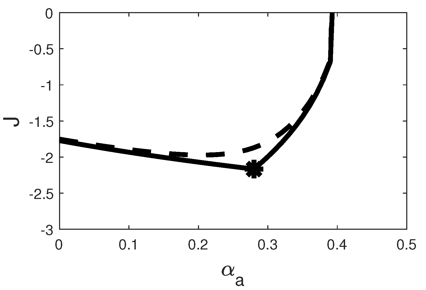
2.3. Constrained Objective

Most of the published studies of optimal control applications to the COVID-19 outbreak require the knowledge of a dynamic model in the form of Equations (1) and some robustness provision to account for parameter uncertainties. In contrast, we aim at proposing a model-free strategy allowing direct social distancing adaptation under realistic decision policies with long observation periods (e.g., several weeks) and long sampling periods. Indeed, the pandemic dynamics evolve with the vaccination rate and efficiency as well as the appearance of new mutant strains, challenging model-based strategies.

In most studies, the focus is put on the fatality or infected case limitations, whereas the objective of the present study is to apply an optimal control policy minimizing social distancing (maximizing ${\alpha }_a$) with the concern of psychological health [3,12,23], under constraints such as hospital bed capacity.

The objective function therefore reads:

$$J=-{\alpha }_a+\psi +\varphi$$

(2)

where $-{\alpha }_a$ represents social distancing while $\psi$ and $\varphi$ are respectively a logarithmic barrier on the infected cases and a penalty constraint on the comfort of social distancing:

$$\begin{array}{cc}\hfill \psi & =-{\eta }_{\psi }ln\left(\frac{I\left(t\right)-I_{ref}}{ϵ}\right),\hfill \end{array}$$

(3a)

$$\begin{array}{cc}\hfill \varphi & ={\eta }_{\varphi }max\left(0,{({\alpha }_{a,ref}-{\alpha }_a)}^3\right)\hfill \end{array}$$

(3b)

where ${\eta }_{\psi }$, ${\eta }_{\varphi }$ and $ϵ$ are design parameters. $I_{ref}$ represents the critical level of infections, corresponding to a number of infected people which might lead to an overflow of intensive care hospitalizations. ${\alpha }_{a,ref}$ is the penalty reference for social distancing, i.e., a level at which people will start feeling psychologically affected.

However, logarithmic barriers may sometimes induce numerical issues during transient phases, and, as recommended in [24], Equation (3a) is approximated by a combined barrier-penalty expression as in:

$${\psi }_B=\left\{\begin{array}{c}\psi ifI\left(t\right)-I_{ref}\ge ϵ\\ 0ifI\left(t\right)-I_{ref}<ϵ\end{array}\right.$$

(4)

which is active in the feasible region $I\left(t\right)-I_{ref}\ge ϵ$ and

$${\psi }_P=\left\{\begin{array}{c}0ifI\left(t\right)-I_{ref}\ge ϵ\\ {\eta }_P\left(I_{ref}-I\left(t\right)+ϵ\right)ifI\left(t\right)-I_{ref}<ϵ\end{array}\right.$$

(5)

which is active in the complementary region and where ${\eta }_P$ is a new design parameter.

Objective 2 is then rewritten as:

$$J=-{\alpha }_a+{\psi }_B+{\psi }_P+\varphi$$

(6)

The chosen parametrization is summarized in

Table 2. Parameter values of the objective function (6).

${\mathit{I}}_{\mathbf{ref}}$	${\mathit{\alpha }}_{\mathit{a},\mathbf{ref}}$$\left[{\mathit{d}}^{-1}\right]$	${\mathit{\eta }}_{\mathit{\psi }}$	${\mathit{\eta }}_{\mathit{\varphi }}$	${\mathit{\eta }}_{\mathit{P}}$	$\mathit{ϵ}$
2	$0.5$	1	1	200	$0.3$

and Figure 1 shows the evolution of (6) as a function of ${\alpha }_a$ after 200 days and once in steady-state.

To solve this minimization problem, a discrete extremum seeking strategy has been proposed in [9], resulting in a two-stage convergence rate, first, quickly catching the transient optimum and greedily tracking [25] its drift towards the steady-state optimum (highlighted by the star in Figure 1). Even if this application was successful, several practical shortcomings were highlighted, such as the inconsistent daily changes and the infinity of possible quantization levels (each of them assimilated to an adopted sanitary policy) of the social distancing variable. In this study, we therefore propose a new problem formulation including these important aspects to make the control policy applicable in a real epidemiological context.

3. Social Distancing Real-Time Optimization

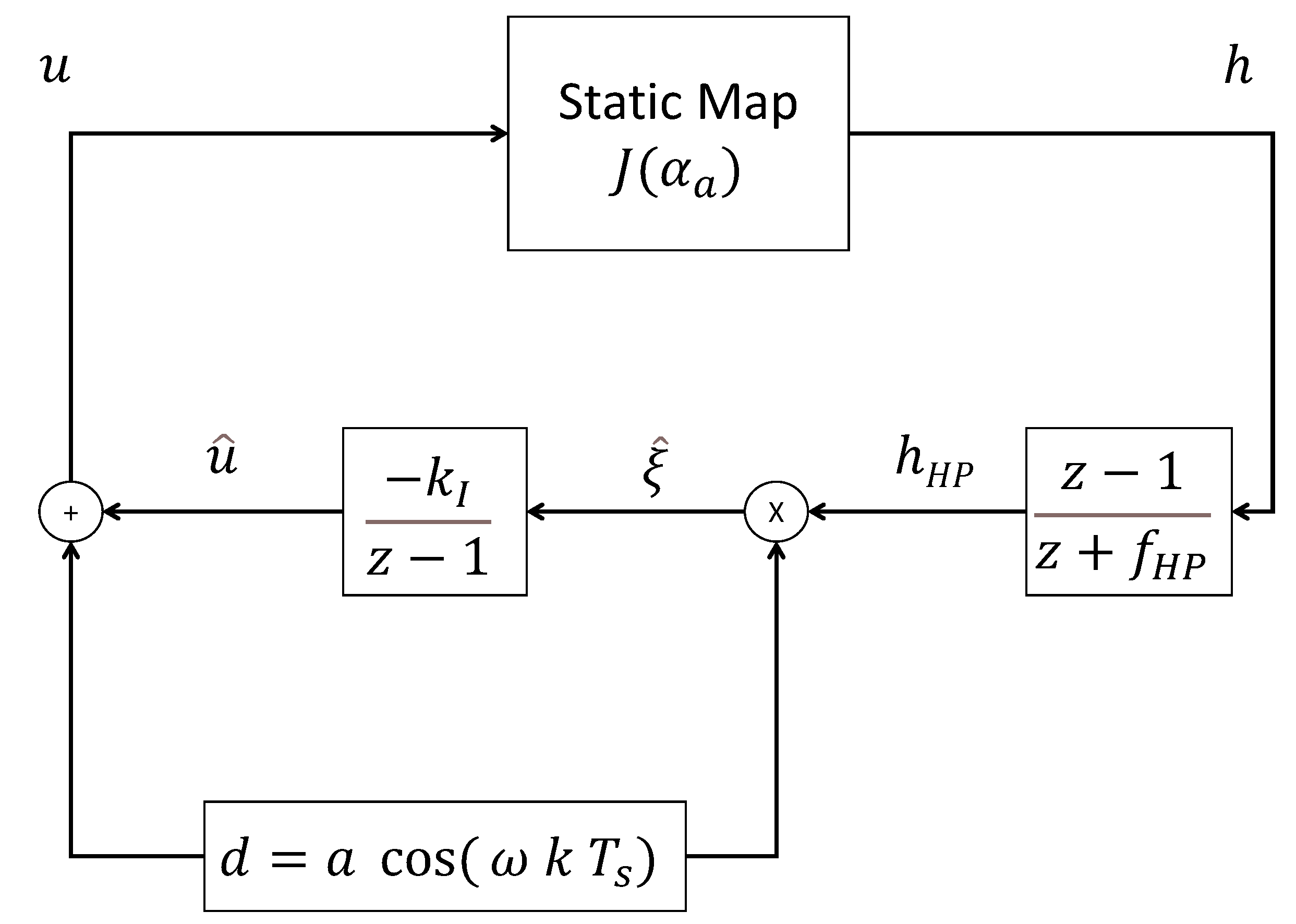
3.1. Classical Discrete-Time Extremum Seeking

Extremum seeking (ES) is a real-time optimization (RTO) strategy driving a system to optimal operating conditions corresponding to the extremum of a measurable convex objective function J [26]. To apply this approach, model 1 and objective function 6 are first cast under the following generic nonlinear state-space form:

$$\begin{array}{cc}\hfill \dot{x}& =f(x,u)\hfill \end{array}$$

(7a)

$$\begin{array}{cc}\hfill y& =Cx\hfill \end{array}$$

(7b)

$$\begin{array}{cc}\hfill J& =h\left(y\right(x),u)\hfill \end{array}$$

(7c)

where $x\in {\Re }^n$ is the state vector, $u\in {\Re }^r$ the input vector, $y\in {\Re }^m$ the output vector, C the $m\times n$ measurement matrix and J the cost function to be minimized.

The convergence of the extremum seeking algorithm is guaranteed if (i) there exists a unique couple of minimizers $x^{*}$ and $u^{*}$ under achievable steady-state conditions, and (ii) if the cost function is convex, fulfilling the necessary condition of optimality [16]. In the COVID-19 pandemic context, a daily reporting of the cases is delivered, and a discrete formulation of the perturbation-based ES is therefore recommended, based on the scheme represented in Figure 2.

The system input is excited by a periodic dither signal and the objective function measurement is high-pass filtered in order to recover the useful information at the dither frequency. The filtered signal, $h_{HP}$, is then demodulated with the same dither signal, providing the cost criterion gradient estimate $\widehat{\xi }=\widehat{\frac{\partial h}{\partial u}}$. Finally, the input signal is recovered from the integration of $\widehat{\xi }$.

The ES loop of Figure 2 is governed by the following equations:

$$\begin{array}{cc}\hfill h_{HP}\left(k\right)& =h\left(k\right)-h_{HP}(k-1)f_{HP},\hfill \end{array}$$

(8a)

$$\begin{array}{cc}\hfill u\left(k\right)& =-k_I\widehat{\xi }(k-1)+u(k-1),\hfill \end{array}$$

(8b)

$$\begin{array}{cc}\hfill \widehat{\xi }\left(k\right)& =acos\left(\omega k{T}_s\right)h_{HP},\hfill \end{array}$$

(8c)

where $f_{HP}$ is the high-pass filter cut-off frequency, $k_I$ the integrator gain, k is the discrete time variable and $T_s$ the sampling period. The reader may refer to [16,26] for additional elements about stability and convergence analyses of discrete ES. Moreover, Ref. [27] also propose further analysis considering state constraints, introducing barrier and penalty functions, such as Equation (3). In the next subsection, to solve the practical shortcomings discussed in Section 2.3 regarding social distancing management, the particular case involving quantization of the actuator level is presented, adapting the strategy of [21].

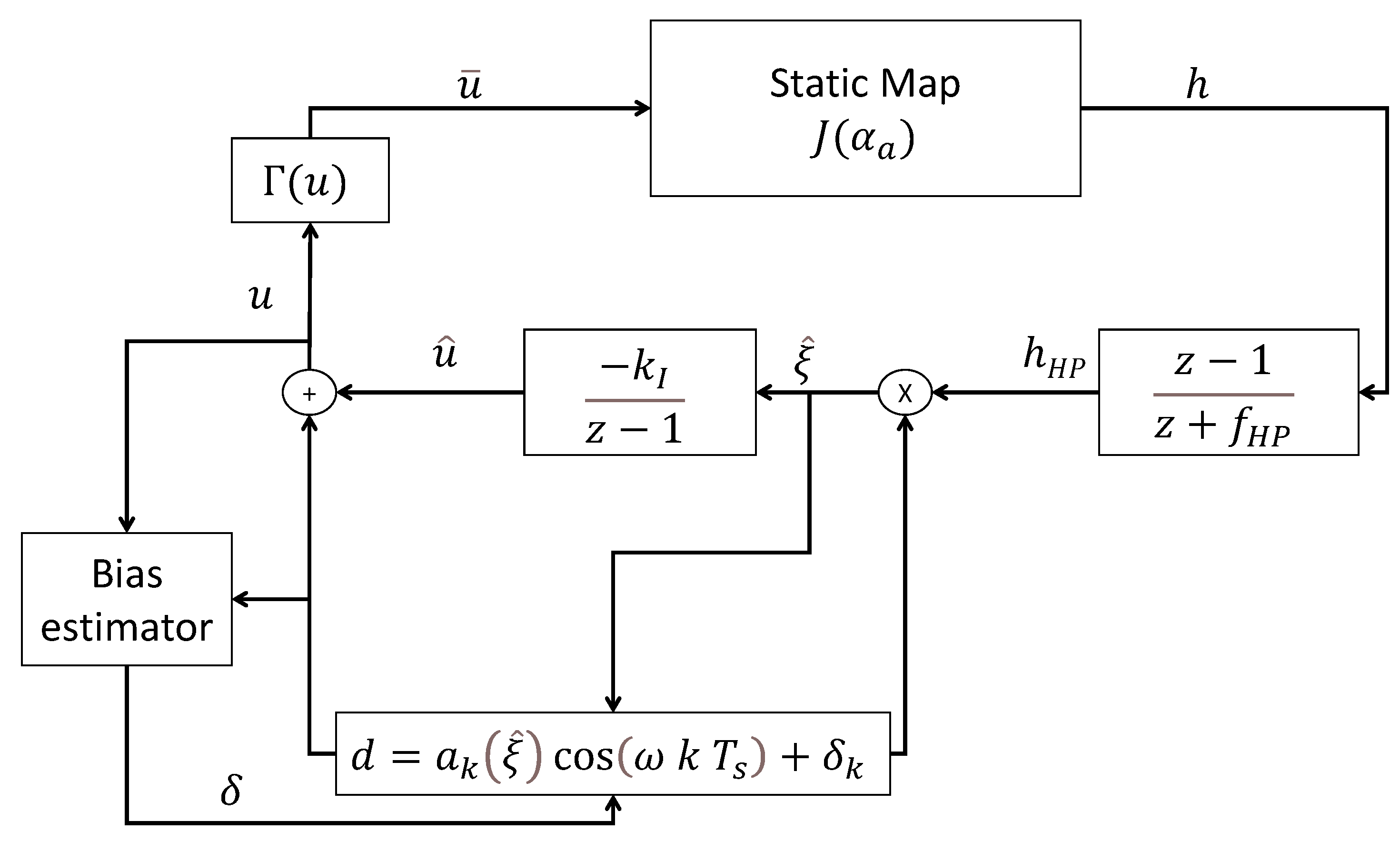
3.2. Discrete-Time Quantized Extremum Seeking

Under specific quantized setting of the actuator over n steps covering the range of admissible values $u_k$ ($k=0,1,\cdots ,n-1$) belonging to the set U, the input can be reformulated as follows:

$$\overline{u}=\Gamma \left(u\right)=\left\{\begin{array}{c}{u}_{-}\mathrm{if}u\le \frac{\left(u_k+u_{k-1}\right)}{2},\\ u_{+}\mathrm{if}u>\frac{\left(u_k+u_{k-1}\right)}{2},\end{array}\right.$$

(9)

where the chosen constant actuator quantum is $u_{+}-u_{-}$. The discrete perturbation-based ES equations become:

$$\begin{array}{cc}\hfill h_{HP}\left(k\right)& =h\left(k\right)-h_{HP}(k-1)f_{HP},\hfill \end{array}$$

(10a)

$$\begin{array}{cc}\hfill \overline{u}\left(k\right)& =\Gamma \left(-k_I\widehat{\xi }(k-1)+\overline{u}(k-1)+d\left(k\right)\right),\hfill \end{array}$$

(10b)

$$\begin{array}{cc}\hfill \widehat{\xi }\left(k\right)& =d\left(k\right)h_{HP}\left(k\right),\hfill \end{array}$$

(10c)

$$\begin{array}{cc}\hfill d\left(k\right)& =acos\left(\omega k{T}_s\right)+\delta \left(k\right)\hfill \end{array}$$

(10d)

and the ES scheme is updated by including the new quantizing blocks as shown in Figure 3.

The bias created by the quantization of the input is comparable to a saturation which should be compensated in order to avoid windup of the ES integral loop and loss of convergence. A signal ${\delta }_k$ is introduced by [21], accounting for the estimation bias in such a way that

$$\underset{\mathrm{k}\to \infty }{\lim }\frac{1}{N}\sum _{i=k}^{k+N-1}\Gamma \left({\widehat{u}}_i+d_i+{\delta }_i\right)=u_k,$$

(11)

where N denotes a horizon over which the input signal is averaged. Equation (11) highlights the role of variable $\delta$ which acts on the input to compensate asymptotically the saturation bias. This variable is updated as follows:

$${\delta }_{k+1}={\delta }_k-\lambda Y_k,$$

(12)

where $\lambda$ is an adaptation gain chosen so as to allow $\delta$ to reach a sufficient level with respect to the dither signal magnitude and

$$Y_k=\Gamma \left(\Gamma \left(-k_I\widehat{\xi }\left(k\right)\right)+d_k+{\delta }_k\right)-\Gamma \left(-k_I\widehat{\xi }\left(k\right)\right),$$

(13)

which measures the deviation between the quantization of the perturbed/compensated gradient (i.e., including the dither and the bias estimation) and its original quantized counterpart.

The magnitude of the dither signal a evolves in relation with the gradient estimate as suggested in [28], until a lower bound $a_{-}$ is reached. This allows the ES algorithm to reduce its oscillations (or even halt if $a_{-}\approx 0$) when reaching a sufficiently close neighborhood of the optimum. It also allows for increasing the dither magnitude if the gradient estimate suggests that a departure from the neighborhood has occurred (for instance, in the presence of external disturbances). It should be noticed that the adaptation of the dither magnitude assumes smoothness of the cost function in the optimum vicinity. Under persistence of excitation (PE), the ES algorithm converges in a close neighborhood of the optimum, function of the dither signal magnitude and frequency. This PE condition is fulfilled with:

$$a_{k+1}=max\left(a_{-},a_k+{\sigma }_a\left({\gamma }_a\frac{2}{\pi }ta{n}^{-1}\left(\left|\widehat{\xi }\right|\right)-a_k\right)\right),$$

(14)

where $\frac{2}{\pi }ta{n}^{-1}\left(\widehat{\xi }\right)$ forces the magnitude a to evolve with the gradient. ${\sigma }_a$ should be set taking into account that the larger the dither magnitude, the faster the ES converges and the smaller the dither magnitude, the more accurate the ES algorithm. The value of ${\gamma }_a$ should then be selected so that gradient variations can be taken into account even if convergence is under progress and the magnitude of the dither signal has already significantly decreased.

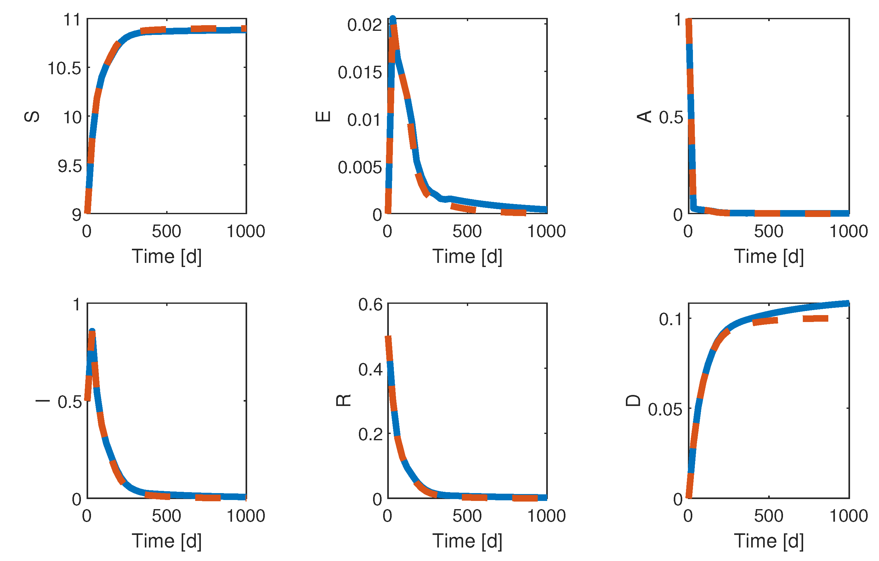
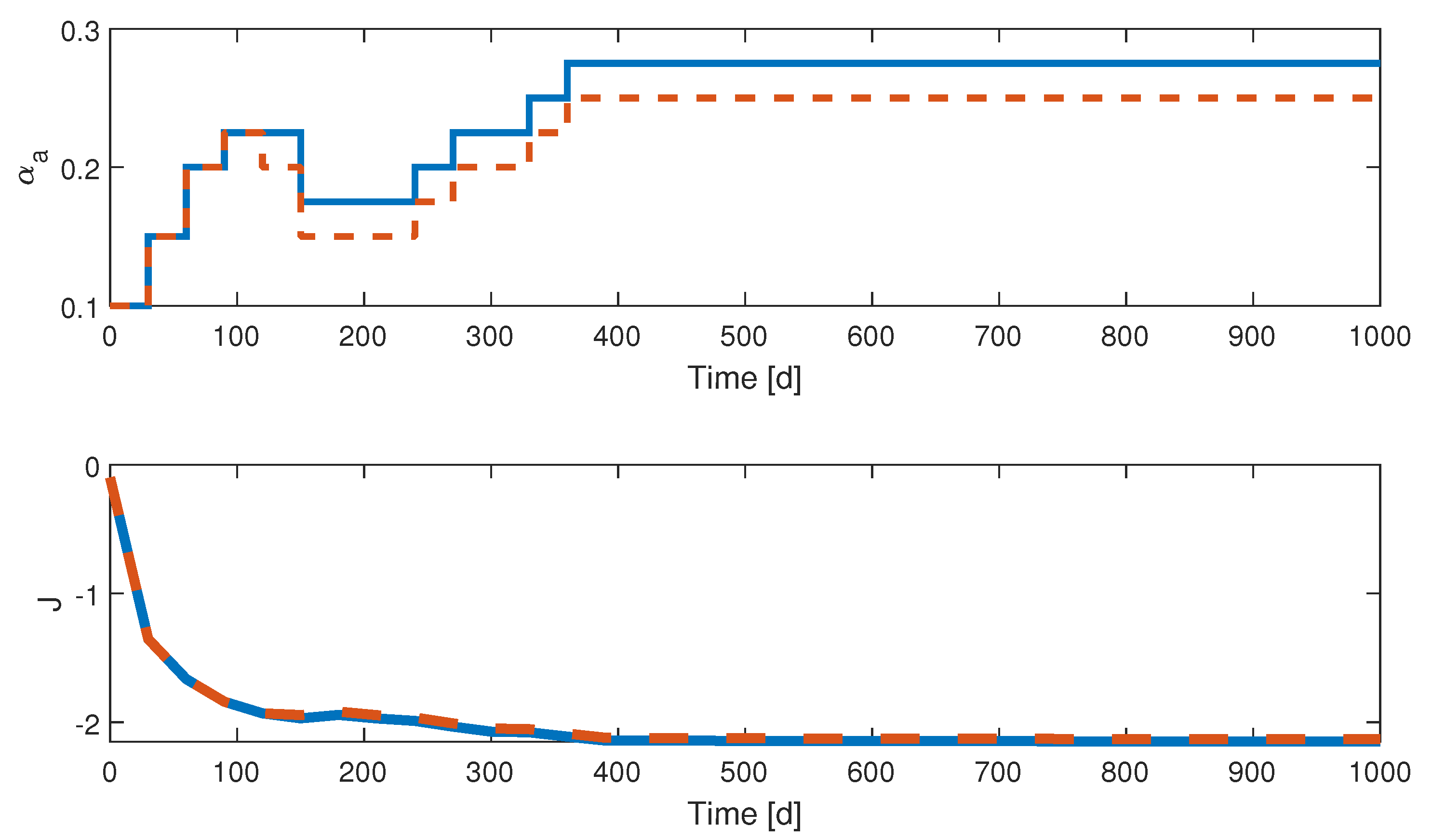
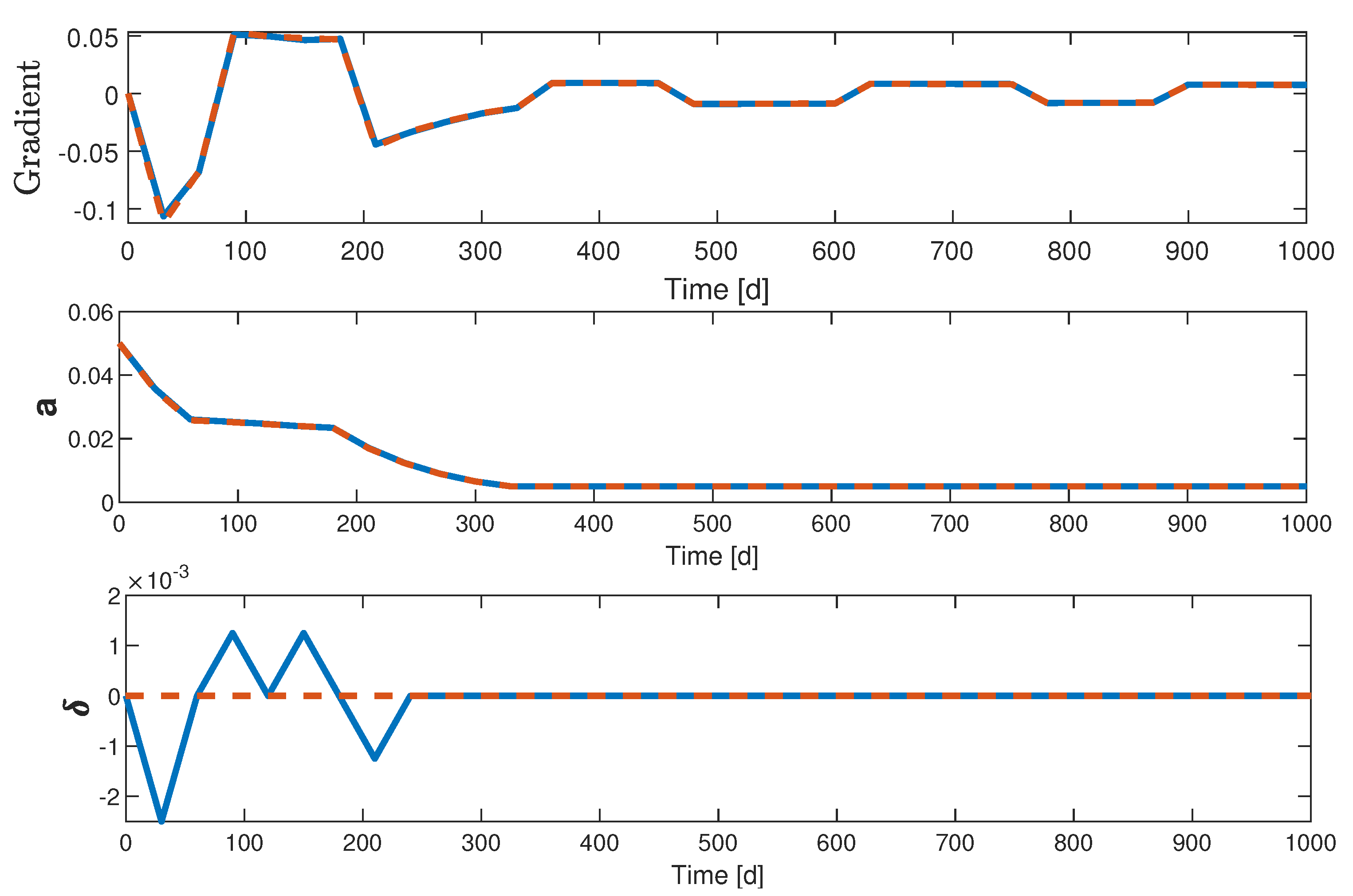
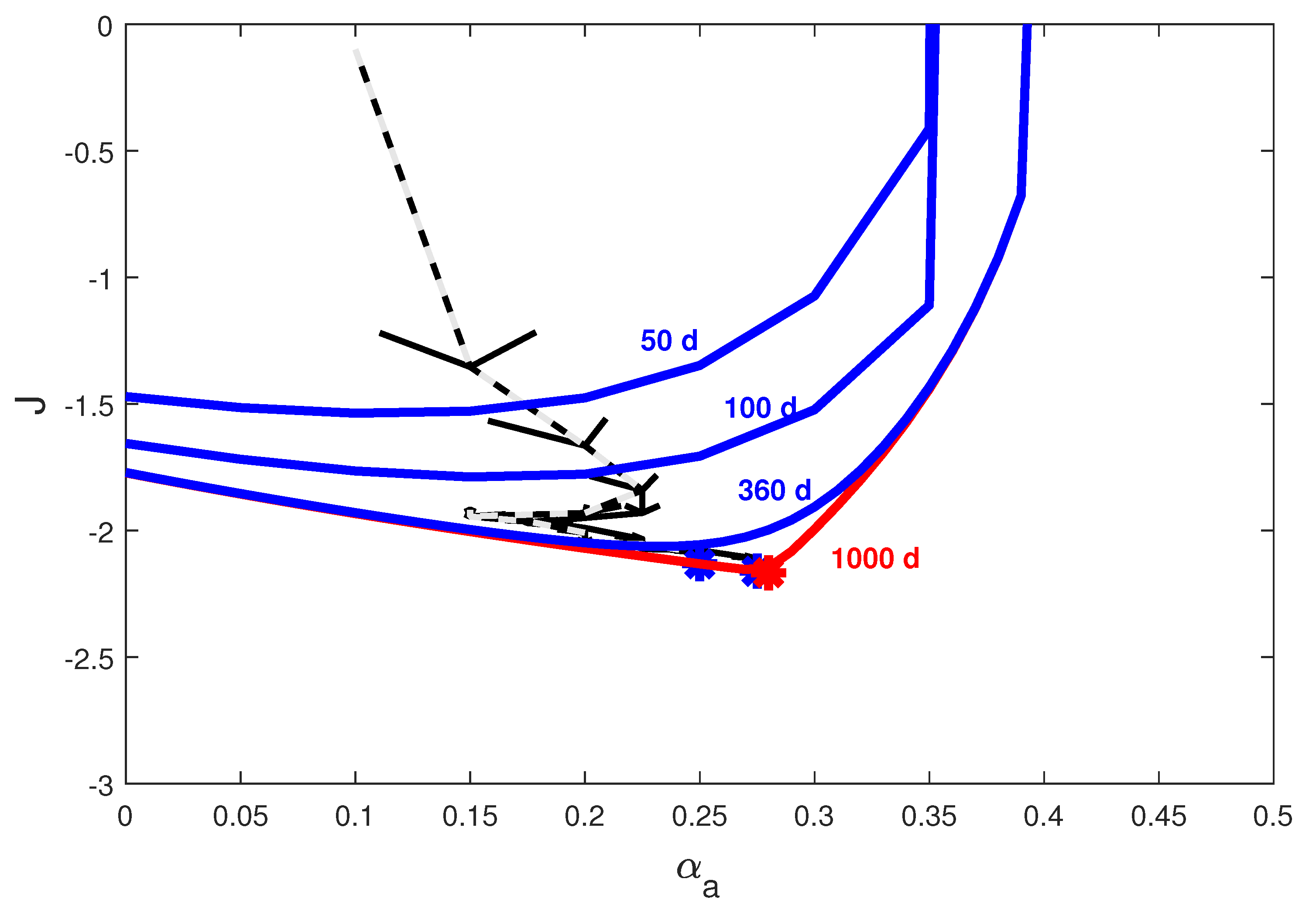
4. Quantized ESC Application to the SEAIR Model

Following the evolution of the sanitary policies in the years 2020–2021 applied by the governments, which have been periodically tighten and relaxed, a quantized ES strategy appears quite instinctive. The application of classical constrained discrete-time ESC to a SEIAR model considering objective function 6 reveals that convergence is achieved in about 100 days to a transient optimum which is drifting with time to a steady-state optimum. The ESC is able to track this optimum in a greedy way over hundreds of days. However, classical ESC considers a daily policy change, which is impractical. The quantized ESC together with a sufficiently long sampling period is a more appropriate approach. In the following, this update period is set to one month (30 days).

The QESC parametrization is based on the guidelines of [21,26,27], and is reported in

Table 3. Parameter values of the ES algorithm.

h$\left[{\mathit{d}}^{-1}\right]$	$\mathit{\omega }$$\left[{\mathit{d}}^{-1}\right]$	${\mathit{a}}_{-}$	${\mathit{a}}_0$	${\mathit{\sigma }}_{\mathit{a}}$	${\mathit{\gamma }}_{\mathit{a}}$	${\mathit{u}}_{+}-{\mathit{u}}_{-}$	${\mathit{k}}_{\mathit{I}}=\frac{1}{{\mathit{\tau }}_{\mathit{I}}}$
$0.99$	$\frac{2\pi }{205}$	$0.005$	$0.05$	$0.15$	$0.7$	$0.025$	$\frac{1}{7}$

.

The following numerical study considers two case studies, either with bias compensation or without (in the latter case, $\delta$ is simply set to zero and never updated). Figure 4, Figure 5, Figure 6 and Figure 7 show the results of the QESC application over 1000 days. In Figure 5, the input evolution in both cases is similar, even though an offset appears after 100 days. The objective function reaches a transient optimum after 100 days, as it was observed in [9], before drifting to the neighborhood of the steady-state optimum after 350 days (about 1 year). We can conclude that constraining the problem by input quantization and longer sampling periods does not deteriorate the convergence time of the ESC strategy and, furthermore, that the bias compensation allows approaching more accurately the steady-state optimum. The adaptation of the dither signal magnitude a behaves as expected since it stops decreasing between 100 and 200 days, when the gradient has, on average, not yet converged to 0. After 200 days, the exponential decrease restarts and, interestingly, the bias compensation variable $\delta$ also stops varying at the same time.

5. Conclusions

This study proposes an original application of quantized extremum seeking control (QESC) to solve the social distancing optimization problem in the framework of the COVID-19 pandemic. The problem formulation aims at minimizing social distancing, preserving population psychological health, while avoiding the number of infections from rising above a specific level defined, for instance, by hospital bed capacities. The proposed strategy does not rely on the a priori knowledge of an epidemiological model and only adapts social distancing on the basis of an objective function measurement. Considering a compartmental SEAIR model as digital simulator of a hypothetical sanitary situation, discrete ES is able to quickly converge to a transient optimum of the objective map which slowly drifts until reaching steady-state. The proposed QESC deals with practical shortcomings such as (i) the dither signal magnitude reduction/extinction when stabilizing at the optimum, (ii) the long observation period following the application of a sanitary policy and the corresponding long sampling period constraint, (iii) the quantization of the decision policy over a limited number of decision levels and (iv) the compensation of the saturation bias. The results show no deterioration of the convergence performance while improving the simplicity of decision-making. Future work includes the combination of quarantining, testing and vaccination as new inputs, requiring strategies like mutivariable ES [16], maximum-likelihood ES [29] or Newton-based ES [30].

References

1. McBryde, E.S.; Meehan, M.T.; Adegboye, O.A.; Adekunle, A.I.; Caldwell, J.M.; Pak, A.; Rojas, D.P.; Williams, B.; Trauer, J.M. Role of modelling in COVID-19 policy development. Paediatr. Respir. Rev. 2020, 35, 57–60. [Google Scholar] [CrossRef]
2. Kermack, W.O.; McKendrick, A.G. A contribution to the mathematical theory of epidemics. Proc. R. Soc. Lond. A 1927, 115, 700–721. [Google Scholar]
3. Tsay, C.; Lejarza, F.; Stadherr, M.; Baldea, M. Modeling, state estimation, and optimal control for the US COVID-19 outbreak. Sci. Rep. 2020, 10, 10711. [Google Scholar] [CrossRef] [PubMed]
4. Köhler, J.; Schwenkel, L.; Koch, A.; Berberich, J.; Pauli, P.; Allgöwer, F. Robust and optimal predictive control of the COVID-19 outbreak. Annu. Rev. Control 2020, 51, 525–539. [Google Scholar] [CrossRef] [PubMed]
5. Péni, T.; Csutak, B.; Szederkényl, G.; Röst, G. Nonlinear model predictive control with logic constraints for COVID-19 management. Nonlinear Dyn. 2020, 102, 1965–1986. [Google Scholar] [CrossRef] [PubMed]
6. Shirin, A.; Lin, Y.; Sorrentino, F. Data-driven optimized control of the COVID-19 epidemics. Sci. Rep. 2021, 11, 6525. [Google Scholar] [CrossRef]
7. Ghamizi, S.; Rwemalika, R.; Cordy, M.; Veiber, L.; Bissyandé, T.F.; Papadakis, M.; Klein, J.; Le Traon, Y. Data-driven Simulation and Optimization for COVID-19 Exit Strategies. In Proceedings of the KDD’20: Proceedings of the 26th ACM SIGKDD Conference on Knowledge Discovery &Data Mining, Virtual Event, CA, USA, 6–10 July 2020; pp. 3434–3442. [Google Scholar]
8. Eker, S. Validity and usefulness of COVID-19 models. Humanit. Soc. Sci. Commun. 2020, 7, 54. [Google Scholar] [CrossRef]
9. Dewasme, L.; Vande Wouwer, A. Fast transient optimization of social distancing during COVID-19 pandemics using extremum seeking. IFAC-PapersOnLine 2021, 54, 145–150. [Google Scholar] [CrossRef]
10. Markovič, R.; Šterk, M.; Marhl, M.; Perc, M.; Gosak, M. Socio-demographic and health factors drive the epidemic progression and should guide vaccination strategies for best COVID-19 containment. Results Phys. 2022, 26, 104433. [Google Scholar] [CrossRef] [PubMed]
11. Krueger, T.; Gogolewski, K.; Bodych, M.; Gambin, A.; Giordano, G.; Cuschieri, S.; Czypionka, T.; Perc, M.; Petelos, E.; Rosińska, M.; et al. Risk assessment of COVID-19 epidemic resurgence in relation to SARS-CoV-2 variants and vaccination passes. Commun. Med. 2022, 2, 23. [Google Scholar] [CrossRef]
12. Dias, S.; Queiroz, K.; Araujo, A. Controlling epidemic diseases based only on social distancing level: General case. ISA Trans. 2022, 124, 21–30. [Google Scholar] [CrossRef] [PubMed]
13. Marques Lopes Santos, D.; Hugo Pereira Rodrigues, V.; Roux Oliveira, T. Epidemiological Control of COVID-19 Through the Theory of Variable Structure and Sliding Mode Systems. J. Control Autom. Electr. Syst. 2021, 33, 63–77. [Google Scholar] [CrossRef]
14. Leblanc, M. Sur l’électrification des chemins de fer au moyen de courants alternatifs de fréquence élevée. Rev. Générale L’Électricité 1922, 12, 275–277. [Google Scholar]
15. Guay, M.; Zhang, T. Adaptive extremum seeking control of nonlinear dynamic systems with parametric uncertainties. Automatica 2003, 39, 1283–1293. [Google Scholar] [CrossRef]
16. Ariyur, K.B.; Krstic, M. Real-Time Optimization by Extremum-Seeking Control, wiley-interscience ed.; John Wiley & Sons, Inc.: Hoboken, NJ, USA, 2003. [Google Scholar]
17. Tan, Y.; Moase, W.; Manzie, C.; Nesic, D.; Mareels, I. Extremum Seeking from 1922 to 2010. In Proceedings of the 29th Chinese Control Conference, Beijing, China, 29–31 July 2010; pp. 14–26. [Google Scholar]
18. Dewasme, L.; Vande Wouwer, A. Model-Free Extremum Seeking Control of Bioprocesses: A Review with a Worked Example. Processes 2020, 8, 1209. [Google Scholar] [CrossRef]
19. Aström, K.J.; Wittenmark, B. Adaptive Control, 2nd ed.; Addison-Wesley Publishing Company, Inc.: Boston, MA, USA, 1995. [Google Scholar]
20. Dewasme, L.; Feudjio Letchindjio, C.G.; Zuniga, I.T.; Vande Wouwer, A. Micro-algae productivity optimization using extremum-seeking control. In Proceedings of the 2017 25th Mediterranean Conference on Control and Automation (MED), Valletta, Malta, 3–6 July 2017; IEEE: Manhattan, NY, USA, 2017; pp. 672–677. [Google Scholar]
21. Guay, M.; Burns, D. Extremum Seeking Control for Discrete-Time with Quantized and Saturated Actuators. Processes 2019, 7, 831. [Google Scholar] [CrossRef]
22. Tan, Y.; Li, Y.; Mareels, I.M.Y. Extremum Seeking for Constrained Inputs. IEEE Trans. Autom. Control 2013, 58, 2405–2410. [Google Scholar] [CrossRef]
23. Elie, R.; Hubert, E.; Turinici, G. Contact rate epidemic control of COVID-19: An equilibrium view. Math. Model. Nat. Phenom. 2020, 15, 35. [Google Scholar] [CrossRef]
24. Srinivasan, B.; Biegler, L.; Bonvin, D. Tracking the necessary conditions of optimality with changing set of active constraints using a barrier-penalty function. Comput. Chem. Eng. 2008, 32, 572–579. [Google Scholar] [CrossRef]
25. Trollberg, O.; Jacobsen, E. Greedy Extremum Seeking Control with Applications to Biochemical Processes. IFAC-PaperOnLine 2016, 49, 109–114. [Google Scholar] [CrossRef]
26. Choi, J.; Krstić, M.; Ariyur, K.; Lee, J. Extremum Seeking Control for Discrete-Time Systems. IEEE Trans. Autom. Control 2002, 47, 318–323. [Google Scholar] [CrossRef]
27. DeHaan, D.; Guay, M. Extremum-seeking control of state-constrained nonlinear systems. Automatica 2005, 41, 1567–1574. [Google Scholar] [CrossRef]
28. Atta, K.; Hostettler, R.; Birk, W.; Johansson, A. Phasor Extremum Seeking Control with Adaptive Perturbation Amplitude. In Proceedings of the 2016 IEEE 55th Conference on Decision and Control (CDC), Las Vegas, NV, USA, 12–14 December 2016; pp. 7069–7074. [Google Scholar]
29. Dewasme, L.; Vande Wouwer, A.; Feudjio Letchindjio, C.; Ahmad, A.; Engell, S. Maximum-likelihood extremum seeking control of microalgae cultures. IFAC-PapersOnLine 2021, 54, 336–341. [Google Scholar] [CrossRef]
30. Ghaffari, A.; Krstić, M.; Nesić, D. Multivariable Newton-based extremum seeking. J. Process Control 2012, 48, 1759–1767. [Google Scholar] [CrossRef]
Figure 1. Evolution of objective function (6) with respect to the input α a , describing the cost of pandemic mitigation with respect to the social distancing level. This figure highlights a unique optimum represented by the black star. Continuous line: steady-state values. Dashed line: transient values after 200 days.
Covid 02 00079 g001
Figure 2. Discrete perturbation-based extremum seeking [26]. The input u is modulated with the dither signal d perturbing the measured objective function h = J . The latter signal is then demodulated in two steps: first by removing the continuous component and low frequencies through a high-pass filter with cut-off frequency f H P , then by multiplying the filtered signal h H P by the dither signal to isolate the information on the gradient ξ ^ at ω . The integration of the gradient estimate provides the input estimate u ^ .
Covid 02 00079 g002
Figure 3. Quantized discrete perturbation-based extremum seeking (adapted from [21]). In comparison with Figure 2, this scheme allows for estimating the bias δ due to the input quantization (saturation) Γ ( u ) , and providing a correction (by addition to the dither signal).
Covid 02 00079 g003
Figure 4. Application of discrete QESC to system (1)—time evolution of the states. In blue: QESC with bias compensation—In dashed red: QESC without bias compensation. Even if the state variables present almost identical transient trajectories, the latter diverge after 200 days and end up in different steady-states. Non-intuitively, converging to a closer neighborhood of the cost objective optimum (i.e., optimizing social distancing) unfortunately leads to slightly higher casualties while still limiting the number of infections.
Covid 02 00079 g004
Figure 5. Application of discrete QESC to system (1): time evolution of the input u = α a and output y = J . Blue line: QESC with bias compensation. Dashed red line: QESC without bias compensation. The impact of bias compensation is highlighted by the faster decrease of the discrete social distancing level (as α a increases) after 200 days.
Covid 02 00079 g005
Figure 6. Application of discrete QESC to system (1): time evolution of the gradient ξ ^ , the dither magnitude a and the bias δ . Blue line: QESC with bias compensation. Dashed red line: QESC without bias compensation. This figure shows the small but important impact of the bias estimation during the transient period, which allows gaining one quantized level on α a as illustrated in Figure 5.
Covid 02 00079 g006
Figure 7. Application of discrete QESC to system (1)—evolution of the output y = J with respect to the input u = α a . Black arrows indicate the convergence direction. Continuous line: QESC with bias compensation. Dashed line: QESC without bias compensation. The blue lines indicate the transient cost functions in 50, 100 and 360 days, while the red line indicates the cost function steady-state after 1000 days. Blue stars show the ending state of the QESC algorithms while the red star indicates the numerical steady-state optimum y * = J * = 2.1665 and u * = α a * = 0.28 . This diagram confirms that, thanks to the bias estimation, the QESC is able to drive the system at the closest quantized level of the optimum J * ( α a * ) .
Covid 02 00079 g007