Comparing the Change in R0 for the COVID-19 Pandemic in Eight Countries Using an SIR Model for Specific Periods


Abstract
1. Introduction
- (1)
- The average length of the non-infectious incubation period: 1 day;
- (2)
- The average length of the infectious incubation period: 3 days;
- (3)
- The average length of the symptomatic period: 7 days;
- (4)
- The ascertainment rate: 0.8.
2. The SIR Model
3. SIR Modelling
- N: Population size;
- : Susceptible (the number of cases in the population who are without immunity against the infection);
- : Infected (the number of cases in the population who are infected);
- : Removed (the number of cases in the population who died or recovered from the infection, or vaccinated with immunity).
- is the transmission rate (the number of effective contacts per day made by an individual);
- is the removal rate (on average, an infected will recover or die in days after infection).
- Case 1: : the epidemic will go on with more and more infected;
- Case 2: : The epidemic will maintain its present condition, with number of infected = number of removed. However, will not stay at one during the course of the epidemic.
- Case 3: : the epidemic will be contained with fewer and fewer cases.
3.1. The R{eSIR} Package
3.2. The tvt.eSIR Method in the R{eSIR} Package
3.3. Initial Values and Hyper-Parameters Used in the tvt.eSIR Function
- (1)
- death_in_R = 0.02(death_in_R refers to the average of cumulative deaths in the removed compartments. When it was within Hubei, 0.4 was used. When it was outside Hubei, 0.02 was used).
- (2)
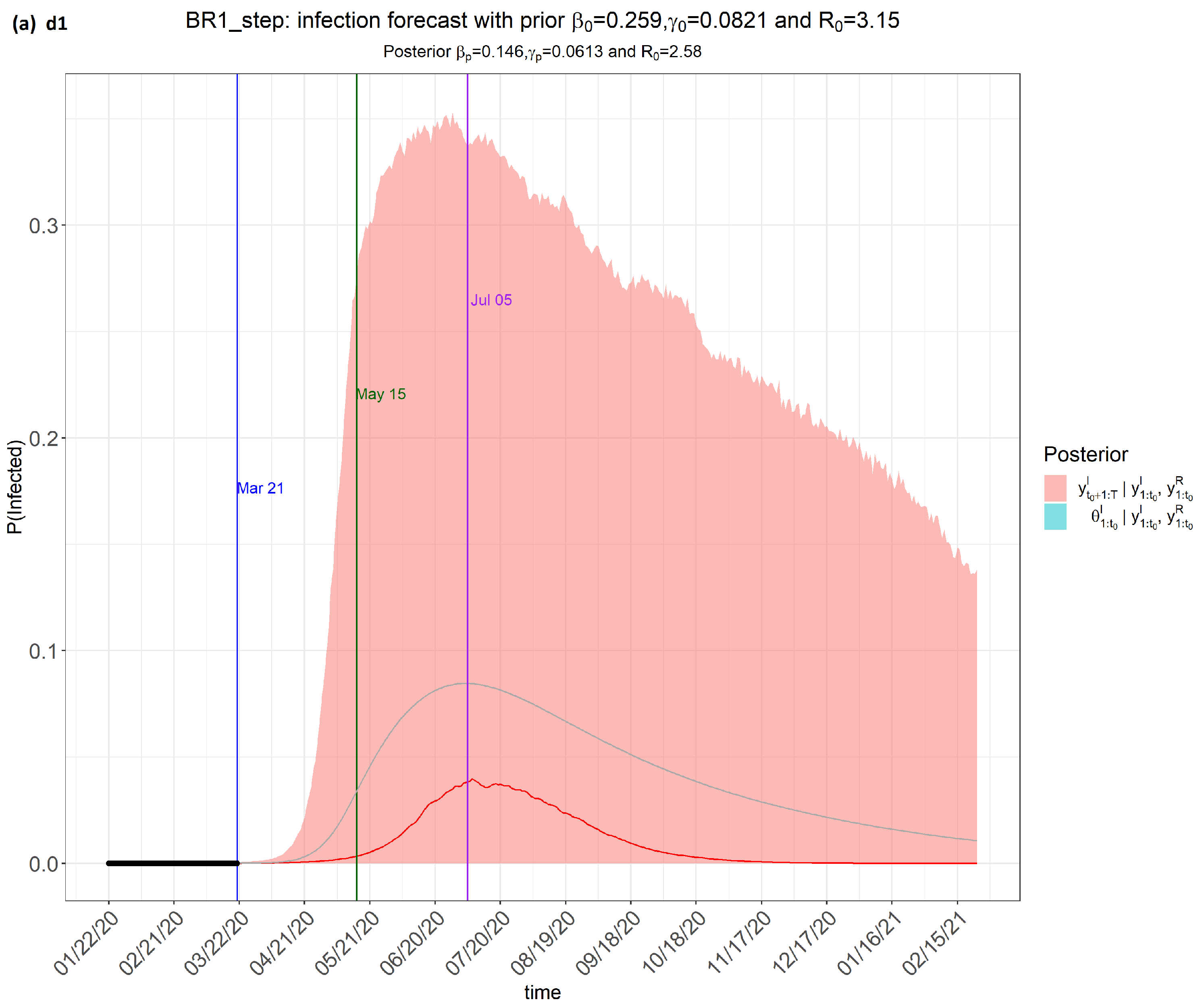
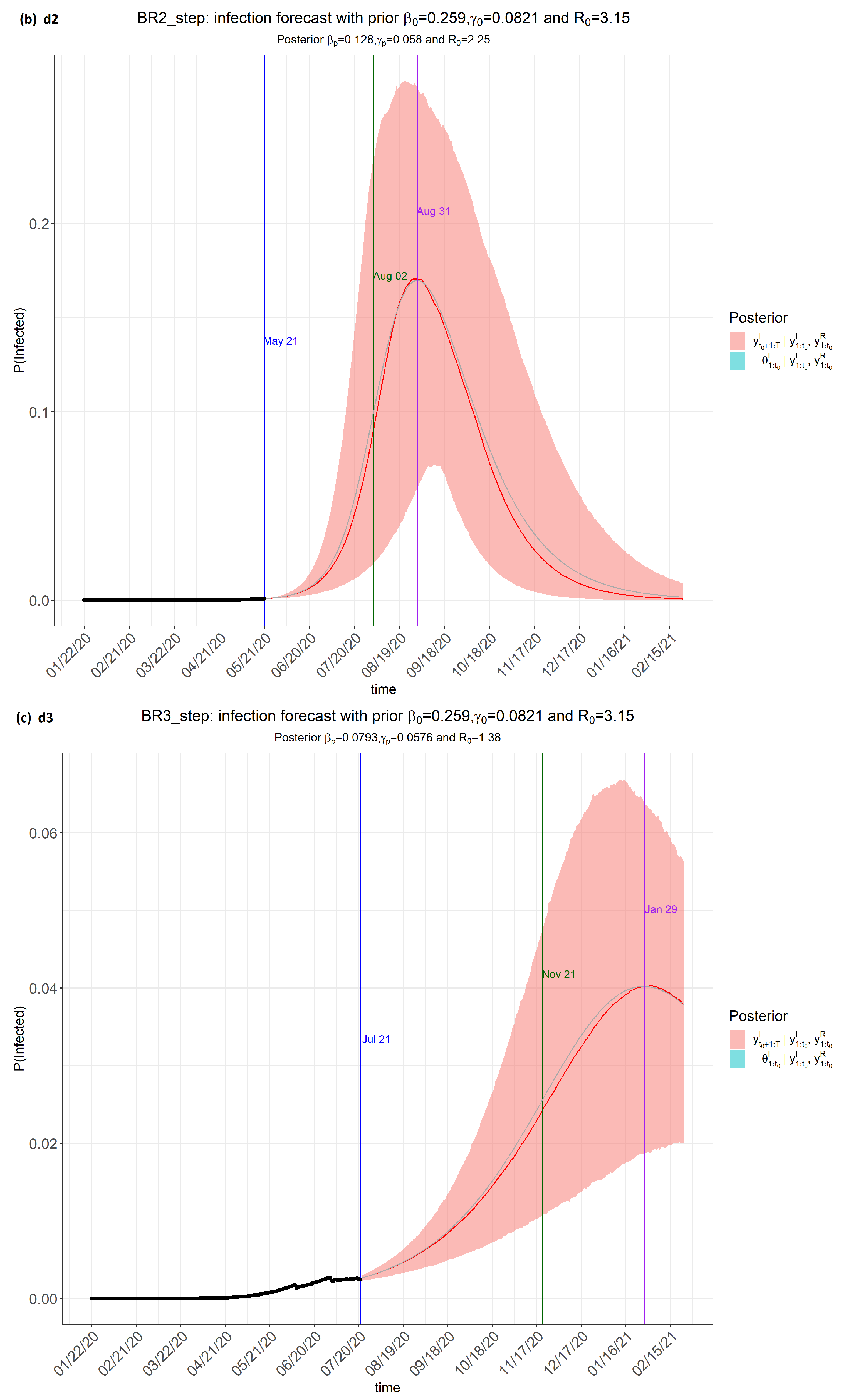
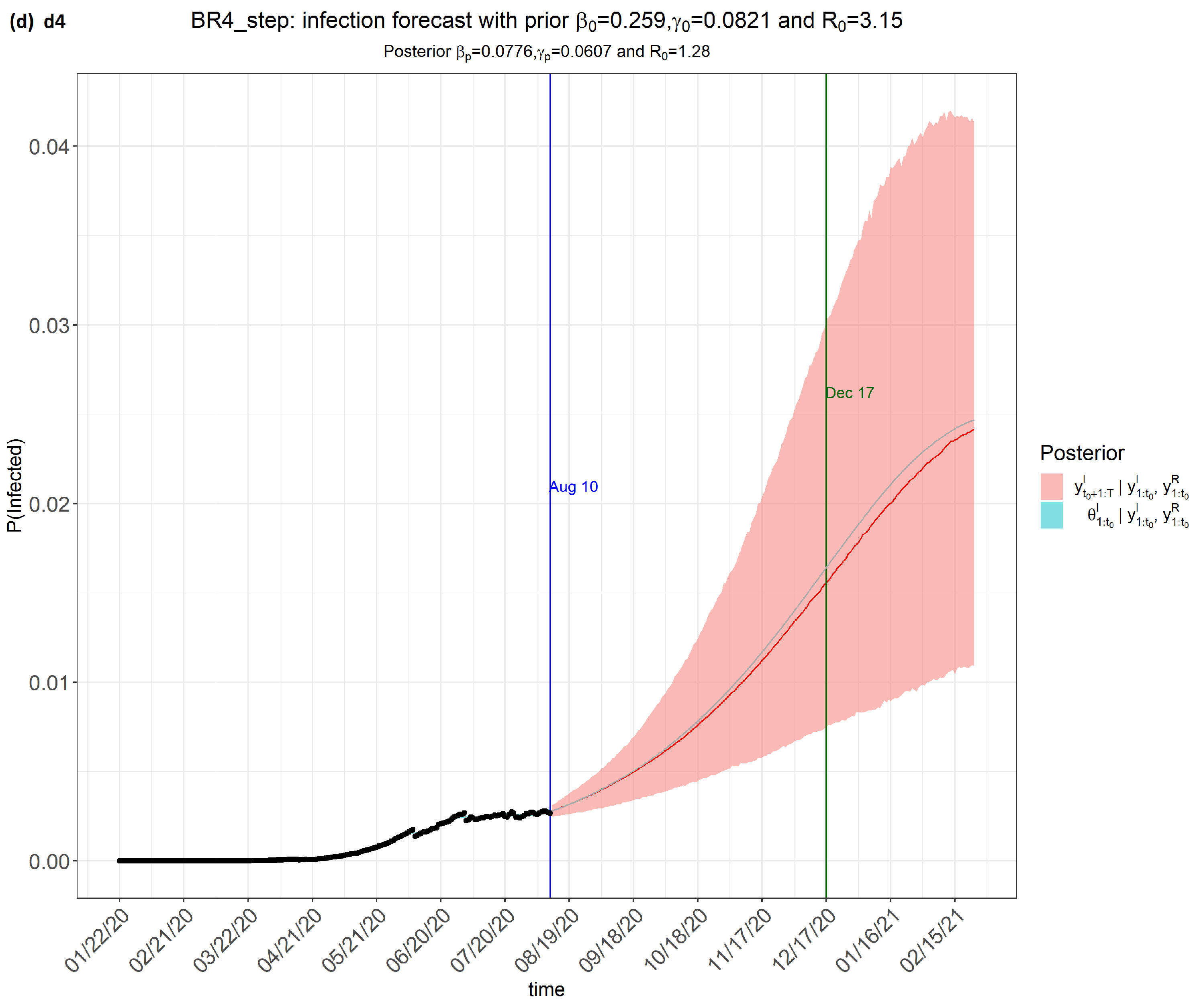
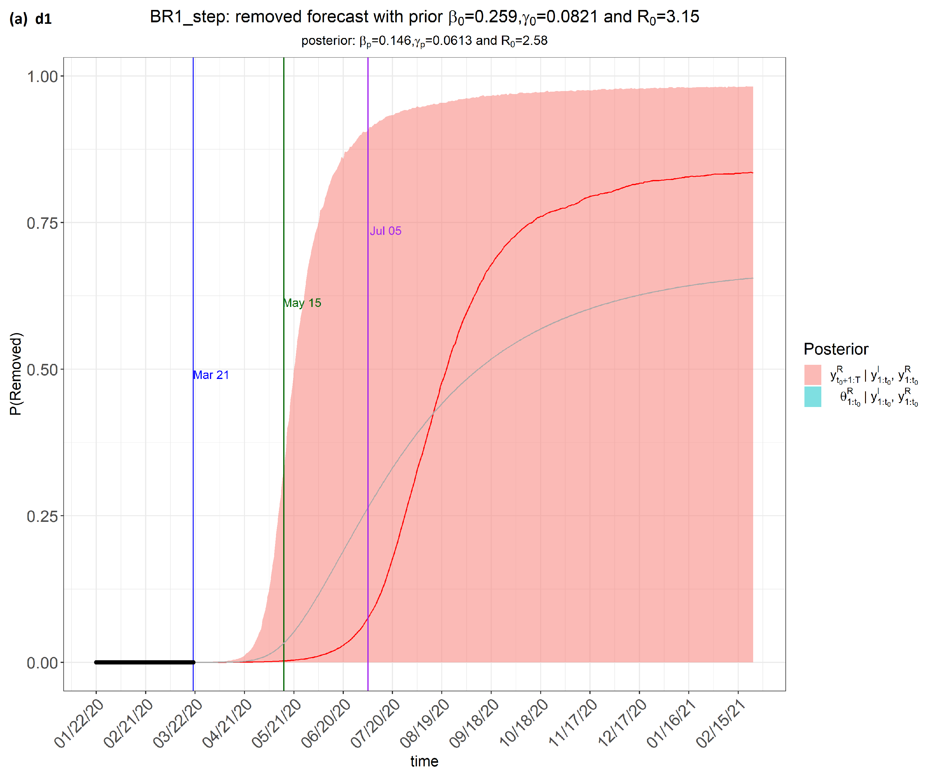
- beta0 = 0.2586(beta0 refers to , the average transmission rate. The value of 0.2586 was estimated from the SARS first-month outbreak [40].
- (3)
- gamma0 = 0.0821(gamma0 refers to , the average removed rate. The value 0.0821 was estimated from the SARS first-month outbreak).
- (4)
- R0 = beta0/gamma0(R0 refers to , the mean reproduction number. With this set of initial values for beta0 and gamma0, = 3.15).
- (5)
- gamma0_sd = 0.1(gamma0_sd refers to the standard deviation for the prior distribution of the removed rate . This value was chosen as a relatively large variance. This allowed more flexibility at the start so as to achieve an easier fit of the data. When more prior knowledge is available, a smaller value can be used for reaching more accurate estimates of parameters).
- (6)
- R0_sd = 1(R0_sd refers to the standard deviation for the prior distribution of . Similarly, this value was chosen as a relatively large variance).
- (7)
- eps = 1 ×(This is a non-zero controller so that all the input Y and R values would be bounded above 1 × .
- (8)
- time_unit = 1 day (It can be set to other values, e.g., 7 days for weekly data. But as the data used in this analysis were the daily numbers, the default of time_unit = 1 day was appropriate).
4. Source of Data
- (1)
- Worldmeter (https://www.worldmeters.info/world-population/population-by-country/(accessed on 22 June 2024));
- (2)
- World Health Organization (https://www.who.int/(accessed on 22 June 2024)); and
- (3)
- Wikipedia (https://www.wikipedia.org/(accessed on 22 June 2024)).
5. Method
- (i)
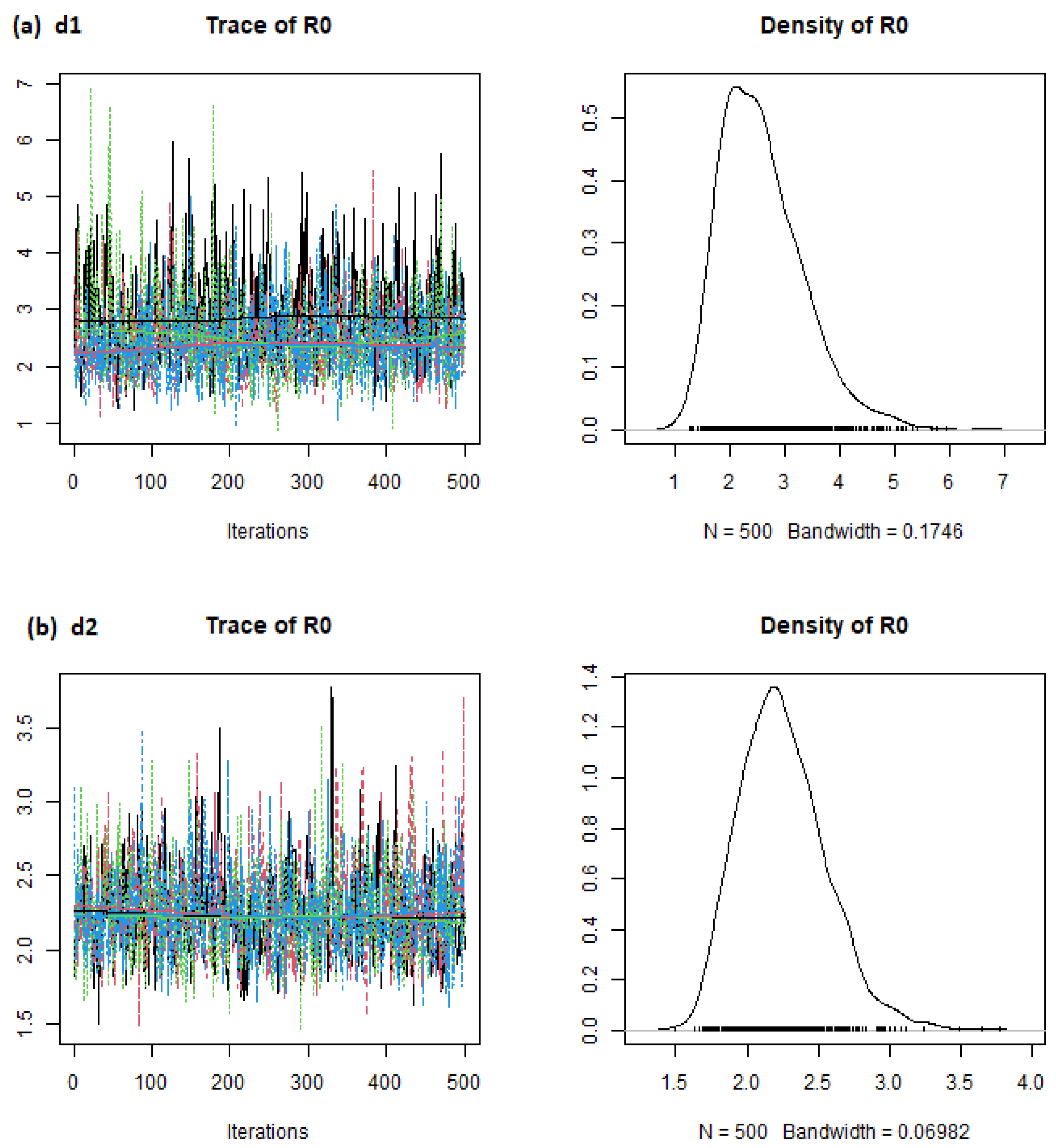
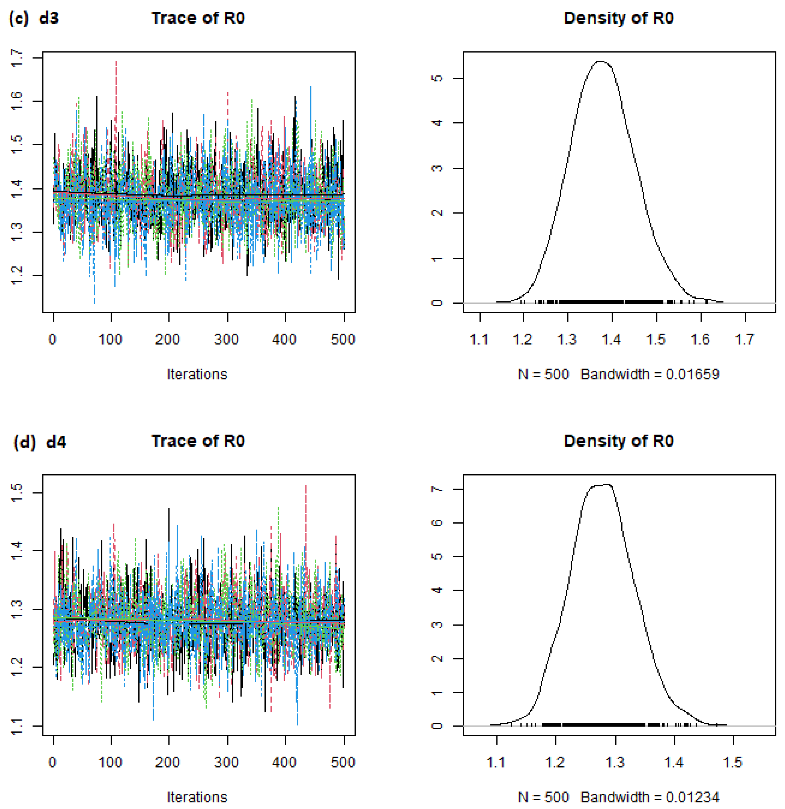
- Time frame 1 (dataset labelled as d1): from 22 January 2020 to 21 March 2020;
- (ii)
- Time frame 2 (dataset labelled as d2): from 22 January 2020 to 21 May 2020;
- (iii)
- Time frame 3 (dataset labelled as d3): from 22 January 2020 to 21 July 2020;
- (iv)
- Time frame 4 (dataset labelled as d4): from 22 January 2020 to 10 August 2020.
6. Results
7. Discussion
Supplementary Materials
Funding
Institutional Review Board Statement
Informed Consent Statement
Data Availability Statement
Conflicts of Interest
Appendix A
References
- Atkeson, A.; Kopecky, K.A.; Zha, T.A. Estimating and Forecasting Disease Scenarios for COVID-19 with an SIR Model; NBER Working Paper: Cambridge, MA, USA, 2020; p. w27335. [Google Scholar]
- Mizumoto, K.; Kagaya, K.; Zarebski, A.; Chowell, G. Estimating the asymptomatic proportion of coronavirus disease 2019 (COVID-19) cases on board the Diamond Princess cruise ship, Yokohama, Japan, 2020. Eur. Cent. Dis. Prev. Control Eurosurveillance 2020, 25, 2000180. [Google Scholar] [CrossRef]
- Donida, B.M. Report on the New Coronavirus COVID-19 Pandemic in Italy; JSciMed Central: Hyderabad, India, 2020. [Google Scholar]
- Zhan, C.; Chi, K.T.; Lai, Z.; Hao, T.; Su, J. Prediction of COVID-19 Spreading Profiles in South Korea, Italy and Iran by Data-Driven Coding; Cold Spring Harbor Laboratory Press: Cold Spring Harbor, NY, USA, 2020. [Google Scholar]
- Sardar, T.; Nadim, S.S.; Rana, S.; Chattopadhyay, J. Assessment of lockdown effect in some states and overall India: A predictive mathematical study on COVID-19 outbreak. Chaos Solitons Fractals 2020, 139, 110078. [Google Scholar] [CrossRef]
- Song, P.X.; Wang, L.; Zhou, Y.; He, J.; Zhu, B.; Wang, F.; Tang, L.; Eisenberg, M. An Epidemiological Forecast Model and Software Assessing Interventions on COVID-19 Epidemic in China; Cold Spring Harbor Laboratory Press: Cold Spring Harbor, NY, USA, 2020. [Google Scholar]
- Arifin, W.N.; Chan, W.H.; Amaran, S.; Musa, K.I. A Susceptible-Infected-Removed (SIR) Model of COVID-19 Epidemic Trend in Malaysia under Movement Control Order (MCO) Using a Data Fitting Approach; Cold Spring Harbor Laboratory Press: Cold Spring Harbor, NY, USA, 2020. [Google Scholar]
- Tolu, L.B.; Ezeh, A.; Feyissa, G.T. How Prepared Is Africa for the COVID-19 Pandemic Response? The Case of Ethiopia. Dove Press Risk Manag. Healthc. Policy 2020, 13, 771. [Google Scholar] [CrossRef] [PubMed]
- Dao, T.L.; Nguyen, T.D. Controlling the COVID-19 pandemic: Useful lessons from Vietnam. Travel Med. Infect. Dis. 2020, 37, 101822. [Google Scholar] [CrossRef] [PubMed]
- Al-Rousan, N.; Al-Najjar, H. Data Analysis of Coronavirus CoVID-19 Epidemic in South Korea Based on Recovered and Death Cases. J. Med. Virol. 2020, 92, 1603–1608. [Google Scholar] [CrossRef] [PubMed]
- Roser, M.; Ritchie, H.; Ortiz-Ospina, E.; Hasell, J. Coronavirus disease (COVID-19)–Statistics and research. Our World Data 2020, 4, 1–45. [Google Scholar]
- Boudrioua, M.S.; Boudrioua, A. Predicting the COVID-19 Epidemic in Algeria Using the SIR Model; Cold Spring Harbor Laboratory Press: Cold Spring Harbor, NY, USA, 2020. [Google Scholar]
- Deo, V.; Chetiya, A.R.; Deka, B.; Grover, G. Forecasting Transmission Dynamics of COVID-19 in India Under Containment Measures-A Time-Dependent State-Space SIR Approach. Stat. Appl. 2020, 18, 157–180. [Google Scholar]
- Juni, P.; Rothenbuhler, M.; Bobos, P.; Thorpe, K.E.; da Costa, B.R.; Fisman, D.N.; Slutsky, A.S.; Gesink, D. Impact of climate and public health interventions on the COVID-19 pandemic: A prospective cohort study. Can. Med. Assoc. J. 2020, 192, E566–E573. [Google Scholar] [CrossRef]
- Bagal, D.K.; Rath, A.; Barua, A.; Patnaik, D. Estimating the Parameters of SIR Model of COVID-19 Cases in India during Lock Down Periods; Cold Spring Harbor Laboratory Press: Cold Spring Harbor, NY, USA, 2020. [Google Scholar]
- Liu, Z.; Magal, P.; Seydi, O.; Webb, G. Understanding unreported cases in the COVID-19 epidemic outbreak in Wuhan, China, and the importance of major public health interventions. Biology 2020, 9, 50. [Google Scholar] [CrossRef]
- Liu, Z.; Magal, P.; Webb, G. Predicting the number of reported and unreported cases for the COVID-19 epidemics in China. arXiv 2020, arXiv:10:2020.04. [Google Scholar]
- Griette, Q.; Demongeot, J.; Magal, P. What can we learn from COVID-19 data by using epidemic models with unidentified infectious cases? medRxiv 2021. 2021-06. Available online: https://www.medrxiv.org/content/10.1101/2021.06.16.21259019v1 (accessed on 6 September 2023).
- Dietz, K.; Heesterbeek, J.A.P. Daniel Bernoulli’s epidemiological model revisited. Math. Biosci. 2002, 180, 1–21. [Google Scholar] [CrossRef] [PubMed]
- Sapna, S.; Tamilarasi, A.; Kumar, M.P. Backpropagation learning algorithm based on Levenberg Marquardt Algorithm. Comp. Sci. Inf. Technol. 2012, 2, 393–398. [Google Scholar]
- Griette, Q.; Demongeot, J.; Magal, P. A robust phenomenological approach to investigate COVID-19 data for France. medRxiv 2021. 2021-02. Available online: https://www.medrxiv.org/content/10.1101/2021.02.10.21251500v1.full (accessed on 6 September 2023). [CrossRef]
- Demongeot, J.; Magal, P. Data-Driven Mathematical Modeling Approaches for COVID-19: A survey. arXiv 2023, arXiv:2309.17087. [Google Scholar]
- Howard, W. The SIR Model and the Foundations of Public Health. 1887. Available online: https://mat.uab.cat/~matmat/ebook2013/V2013n03-ebook.pdf (accessed on 6 September 2023).
- Roberts, M.G.; Heesterbeek, J. Mathematical Models in Epidemiology; EOLSS: Abu Dhabi, United Arab Emirates, 2003. [Google Scholar]
- Brauer, F. Compartmental models in epidemiology. Math. Epidemiol. 2008, 1945, 19–79. [Google Scholar]
- Jiang, F.; Zhao, Z.; Shao, X. Time series analysis of COVID-19 infection curve: A change-point perspective. J. Econom. 2020, 232, 1–17. [Google Scholar] [CrossRef]
- Prasse, B.; Achterberg, M.A.; Ma, L.; Van, M.P. Network-inference-based prediction of the COVID-19 epidemic outbreak in the Chinese province Hubei. Appl. Netw. Sci. 2020, 5, 1–11. [Google Scholar] [CrossRef]
- Sahneh, F.D.; Vajdi, A.; Shakeri, H.; Fan, F.; Scoglio, C. GEMFsim: A stochastic simulator for the generalized epidemic modeling framework. J. Comput. Sci. 2017, 22, 36–44. [Google Scholar] [CrossRef]
- Ng, T.W.; Turinici, G.; Danchin, A. A double epidemic model for the SARS propagation. BMC Infect. Dis. 2003, 3, 19. [Google Scholar] [CrossRef]
- Schlickeiser, R.; Kröger, M. Mathematics of Epidemics: On the General Solution of SIRVD, SIRV, SIRD, and SIR Compartment Models. Mathematics 2024, 12, 941. [Google Scholar] [CrossRef]
- Kröger, M.; Schlickeiser, R. On the Analytical Solution of the SIRV-Model for the Temporal Evolution of Epidemics for General Time-Dependent Recovery, Infection and Vaccination Rates. Mathematics 2024, 12, 326. [Google Scholar] [CrossRef]
- Yang, W.; Zhang, D.; Peng, L.; Zhuge, C.; Hong, L. Rational evaluation of various epidemic models based on the COVID-19 data of China. Epidemics 2021, 37, 100501. [Google Scholar] [CrossRef]
- Meng, X.; Zhao, S.; Feng, T.; Zhang, T. Dynamics of a novel nonlinear stochastic SIS epidemic model with double epidemic hypothesis. J. Math. Anal. Appl. 2016, 433, 227–242. [Google Scholar] [CrossRef]
- Wangping, J.; Ke, H.; Yang, S.; Wenzhe, C.; Shengshu, W.; Shanshan, Y.; Yao, H. Extended SIR prediction of the epidemics trend of COVID-19 in Italy and compared with Hunan, China. Front. Front. Med. 2020, 7, 169. [Google Scholar]
- Lin, J. On the Dirichlet Distribution; Department of Mathematics and Statistics, Queens University: Kingston, ON, Canada, 2016. [Google Scholar]
- Manouchehri, N.; Bouguila, N. Multivariate Beta-Based Hierarchical Dirichlet Process Hidden Markov Models in Medical Applications. In Hidden Markov Models and Applications; Springer International Publishing: Cham, Switzerland, 2022; pp. 235–261. [Google Scholar]
- Rößler, A. Runge–Kutta methods for the strong approximation of solutions of stochastic differential equations. SIAM J. Numer. Anal. 2010, 48, 922–952. [Google Scholar] [CrossRef]
- Plummer, M. JAGS, Version 3.3; 0 User Manual; 2012. Available online: https://www.stat.cmu.edu/~brian/463-663/week10/articles (accessed on 6 September 2023).
- Chernozhukov, V.; Hong, H. An MCMC approach to classical estimation. J. Econom. 2003, 115, 293–346. [Google Scholar] [CrossRef]
- Riley, S.; Fraser, C.; Donnelly, C.A.; Ghani, A.C.; Abu-Raddad, L.J.; Hedley, A.J.; Anderson, R.M. Transmission dynamics of the etiological agent of SARS in Hong Kong: Impact of public health interventions. Science 2003, 300, 1961–1966. [Google Scholar] [CrossRef]
- Achaiah, N.C.; Subbarajasetty, S.B.; Shetty, R.M. R0 and re of COVID-19: Can we predict when the pandemic outbreak will be contained? Indian Soc. Crit. Care Med. Indian J. Crit. Care Med.-Peer-Rev. Off. Publ. Indian Soc. Crit. Care Med. 2020, 24, 1125. [Google Scholar] [CrossRef] [PubMed]
- de Souza, W.M.; Buss, L.F.; Candido, D.S.; Carrera, J.P.; Li, S.; Zarebski, A.E.; Pereira, R.H.M.; Prete, C.A., Jr.; de Souza-Santos, A.A.; Parag, K.V.; et al. Epidemiological and clinical characteristics of the COVID-19 epidemic in Brazil. Nat. Hum. Behav. 2020, 4, 856–865. [Google Scholar] [CrossRef] [PubMed]
- Liu, Y.; Gayle, A.A.; Wilder-Smith, A.; Rocklöv, J. The Reproductive Number of COVID-19 is Higher Compared to SARS Coronavirus; Oxford University Press (OUP): Oxford, UK, 2020. [Google Scholar]
- Shil, P.; Atre, N.M.; Patil, A.A.; Tandale, B.V.; Abraham, P. District-wise estimation of Basic reproduction number (R 0) for COVID-19 in India in the initial phase. Spat. Inf. Res. 2021, 30, 1–9. [Google Scholar] [CrossRef]
- Ke, R.; Romero-Severson, E.; Sanche, S.; Hengartner, N. Estimating the reproductive number R0 of SARS-CoV-2 in the United States and eight European countries and implications for vaccination. J. Theor. Biol. 2021, 517, 110621. [Google Scholar] [CrossRef] [PubMed]
- Tariq, A.; Lee, Y.; Roosa, K.; Blumberg, S.; Yan, P.; Ma, S.; Chowell, G. Real-time monitoring the transmission potential of COVID-19 in Singapore, March 2020. BioMed Cent. BMC Med. 2020, 18, 1–14. [Google Scholar] [CrossRef] [PubMed]
- Shim, E.; Tariq, A.; Choi, W.; Lee, Y.; Chowell, G. Transmission potential and severity of COVID-19 in South Korea. Int. J. Infect. Dis. 2020, 93, 339–344. [Google Scholar] [CrossRef]
- Delamater, P.L.; Street, E.J.; Leslie, T.F.; Yang, Y.T.; Jacobsen, K.H. Complexity of the basic reproduction number (R0). Centers Dis. Control Prev. Emerg. Infect. Dis. 2019, 25, 1. [Google Scholar] [CrossRef]


| Country | d1 Mean | d2 Mean | d3 Mean | d4 Mean |
|---|---|---|---|---|
| Brazil | 1.28 | 1.18 | 1.28 | 1.39 |
| China | 2.31 | 1.46 | 2.22 | 3.66 |
| India | 1.49 | 1.26 | 1.48 | 1.76 |
| Italy | 1.19 | 0.97 | 1.18 | 1.45 |
| Singapore | 1.53 | 1.15 | 1.52 | 1.99 |
| South Korea | 2.24 | 1.37 | 2.20 | 3.41 |
| United Kingdom | 3.70 | 2.59 | 3.62 | 5.28 |
| United States of America | 2.63 | 2.23 | 2.62 | 3.10 |
Disclaimer/Publisher’s Note: The statements, opinions and data contained in all publications are solely those of the individual author(s) and contributor(s) and not of MDPI and/or the editor(s). MDPI and/or the editor(s) disclaim responsibility for any injury to people or property resulting from any ideas, methods, instructions or products referred to in the content. |
© 2024 by the author. Licensee MDPI, Basel, Switzerland. This article is an open access article distributed under the terms and conditions of the Creative Commons Attribution (CC BY) license (https://creativecommons.org/licenses/by/4.0/).
Share and Cite
Leung, T.C. Comparing the Change in R0 for the COVID-19 Pandemic in Eight Countries Using an SIR Model for Specific Periods. COVID 2024, 4, 930-951. https://doi.org/10.3390/covid4070065
Leung TC. Comparing the Change in R0 for the COVID-19 Pandemic in Eight Countries Using an SIR Model for Specific Periods. COVID. 2024; 4(7):930-951. https://doi.org/10.3390/covid4070065
Chicago/Turabian StyleLeung, Tak Ching. 2024. "Comparing the Change in R0 for the COVID-19 Pandemic in Eight Countries Using an SIR Model for Specific Periods" COVID 4, no. 7: 930-951. https://doi.org/10.3390/covid4070065
APA StyleLeung, T. C. (2024). Comparing the Change in R0 for the COVID-19 Pandemic in Eight Countries Using an SIR Model for Specific Periods. COVID, 4(7), 930-951. https://doi.org/10.3390/covid4070065