The GUM Tree Calculator: A Python Package for Measurement Modelling and Data Processing with Automatic Evaluation of Uncertainty

Abstract

There is currently interest in the digitalisation of metrology because technologies that can measure, analyse, and make critical decisions autonomously are beginning to emerge. The notions of metrological traceability and measurement uncertainty should be supported, following the recommendations in the Guide to the Expression of Uncertainty in Measurement (GUM). However, GUM offers no specific guidance. Here, we report on a Python package that implements algorithmic data processing using ‘uncertain numbers’, which satisfy the general criteria in GUM for an ideal format to express uncertainty. An uncertain number can represent a physical quantity that has not been determined exactly. Using uncertain numbers, measurement models can be expressed clearly and succinctly in terms of the quantities involved. The algorithms and simple data structures we use provide an example of how metrological traceability can be supported in digital systems. In particular, uncertain numbers provide a format to capture and propagate detailed information about quantities that influence a measurement along the various stages of a traceability chain. More detailed information about influence quantities can be exploited to extract more value from results for users at the end of a traceability chain.

1. Introduction

The worldwide dissemination of Système International (SI) units is a person-oriented paper-based process that is carefully managed by national bodies and coordinated by international organisations; however, that is about to change. The emergence of technologies that can measure and make critical decisions autonomously requires more of our measurement infrastructure to be implemented by digital systems. A growing number of initiatives are replacing paper-based, expert-oriented processes with automated digital ones (e.g., machine-readable formats for calibration reports [1] and a secure cloud-based platform for the legal metrology infrastructure in Europe [2]). Dissemination of SI provides what the metrology community calls traceability. Metrological traceability ensures that measurements are accompanied by information that can be used to determine the fitness-for-purpose of results in different situations. Traceability may be thought of as support for interoperability with measurement data but at present the expertise of skilled individuals is needed to interpret data and supporting information correctly. One outcome of digitalisation will be an ability to produce traceable measurement results in machine-actionable formats.

Measurement accuracy is fundamental to traceability. Traceable measurements must report information about the likely magnitude of the difference (error) between a measured value and the quantity intended to be measured. Metrologists refer to this as measurement uncertainty. During the 1980s, considerable effort went into harmonising the manner that measurement uncertainty is evaluated and communicated and this resulted in the publication of the Guide to the Expression of Uncertainty in Measurement (GUM) [3], which remains today the primary reference for dealing with measurement uncertainty (the GUM was produced by a group of experts representing eight international scientific and technical organisations: the BIPM, IEC, IFCC, ILAC, ISO, IUPAC, IUPAP, and OIML).

Digitalisation of metrological infrastructure will inevitably need algorithmic implementations for GUM methods. However, the GUM itself offers no specific guidance, as it was written long before this need could have been anticipated. One approach, called uncertain numbers, provides an abstract representation for physical quantities that satisfies general criteria in the GUM for an ideal format to express uncertainty [4]. Quantities in a problem, such as specific lengths, masses, etc., are always considered to have definite values that can only be estimated with limited accuracy by measurement. Therefore, an uncertain number is designed to encapsulate information about the measured value and measurement accuracy. Using this abstraction allows data processing to be expressed algorithmically in terms of the quantities involved, leaving the associated uncertainty calculations to be handled automatically in the background. The uncertain-number approach can capture the effects of influence quantities at different stages of a traceable measurement and propagate this information along the chain to an end user. Detailed information about the uncertainty budget can sometimes be used to enhance the value of results. This report describes a Python package, called the GUM Tree Calculator (GTC), that uses uncertain numbers [5]. GTC is a very flexible tool that has been used in two quite different applications, which have been reported on recently [6,7]. We discuss the tool’s design and comment on aspects that support traceability in digital systems.

The next section provides an overview of GUM uncertainty calculations, metrological traceability, and GTC software. GTC is tested on a variety of platforms and different versions of Python 2 and 3 (refer to the github repository [5]). All code snippets use GTC version 1.3.6. The GUM presents its approach to evaluating measurement uncertainty in mathematical terms; thus, Section 2.1 summarises the key equations. However, an alternative formulation of these equations is more practical. This is described in Section 2.2, which motivates the development of the uncertain-number data type. The notion of metrological traceability is discussed in Section 2.3, and we explain why the uncertain-number format is useful to support traceability. Section 2.4 presents an example of GTC data processing applied to an electrical circuit. Section 3 looks in more detail at aspects of GTC design. The method used to automate uncertainty calculation is presented in Section 3.1. The data structures that support uncertainty propagation in uncertain-number objects are described in Section 3.2, Section 3.3, Section 3.4 and Section 3.5; then, Section 3.6 describes how uncertain numbers can be saved and restored. More general considerations are discussed in Section 4. Appendix A briefly describes support for complex quantities, extensions for handling degrees of freedom, and some additional implementation details.

Notation

Upper and lower case letters are used to distinguish between quantities, which will never be determined exactly, and values that will be known (such as a numerical indication on a measuring instrument), respectively. For example, a measurement result y is written in lower-case because a result always has a definite numerical value: The value y is an estimate of Y, which is the quantity intended to be measured. Upper-case is used for Y to indicate that the quantity cannot be known exactly. It is helpful to make this distinction because uncertain-number objects are used to represent quantities; the associated numerical estimates and other known values, such as uncertainty, will appear as attributes of uncertain numbers.

2. Overview

2.1. GUM Method

Measurements are always influenced by unpredictable factors, so a result can only ever approximate the quantity of interest. Influence factors can, however, be identified and described in probabilistic terms. In this manner, a measurement process can be represented by a mathematical model. This is the approach taken in the GUM.

The first step is to identify a function called the measurement model that contains every quantity, including all corrections and correction factors that can contribute a significant component of uncertainty to the measurement result [3] [Section 4.1.2]. In the GUM, this is expressed as an explicit function:

$$Y=f(X_1,X_2,\cdots ,X_l),$$

(1)

where Y is the quantity intended to be measured (the measurand) and the input arguments $X_1,X_2,\cdots ,X_l$ are quantities that influence the measurement outcome. All arguments of $f(\cdots )$ are treated in the same way when evaluating uncertainty. Some of the input terms may represent other measured quantities. For example, electrical resistance could be measured by first measuring potential difference V and current I and then evaluating ratio $R=V/I$. Other input terms may represent nuisance factors that perturb the measurement, such as Johnson noise in a resistor. The measurement model can be thought of as a recipe for evaluating the measurand: if $X_1,X_2,\cdots ,X_l$ were all known exactly, then Y could be determined. However, with only approximate values available for input quantities, an approximate value for Y will be obtained.

$$y=f(x_1,x_2,\cdots ,x_l).$$

(2)

GUM uses a specific term, standard uncertainty, in relation to the unpredictability of measurement outcomes (i.e., the fact that y and Y differ by an unpredictable amount). A standard uncertainty is an estimate of the standard deviation of a probability distribution for the difference (error) between y and Y. There is a formula in the GUM to propagate standard uncertainties through a measurement model and obtain the standard uncertainty in a result. For a model in the form of Equation (1), the standard uncertainty of y, as an estimate of Y, is calculated as follows:

$$u\left(y\right)={\left[\sum _{i=1}^l\sum _{j=1}^l{u}_i\left(y\right)r(x_i,x_j)u_j\left(y\right)\right]}^{1/2},$$

(3)

where $u_i\left(y\right)$ and $u_j\left(y\right)$ are components of uncertainty that relate small changes in input values to corresponding changes in y.

$$u_i\left(y\right)={\left.\frac{\partial Y}{\partial X_i}\right|}_{X_i=x_i}u\left(x_i\right)\mathrm{and}{u}_j\left(y\right)={\left.\frac{\partial Y}{\partial X_j}\right|}_{X_j=x_j}u\left(x_j\right).$$

(4)

The terms $u\left(x_i\right)$ and $u\left(x_j\right)$ are the standard uncertainties in the input values $x_i$ and $x_j$, respectively. The correlation coefficient attributed to a pair of input estimates is $r(x_i,x_j)$, where $r(x_i,x_i)=1$ when $i=j$.

Standard uncertainties are associated with a number called the degrees of freedom, usually denoted $\nu$. The interpretation given to x, $u\left(x\right)$, and $\nu$ in the GUM is analogous to familiar sample statistics: the sample mean, the standard error in the sample mean, and the degrees of freedom [8] [Chapter 9]. However, degrees of freedom are interpreted more broadly in the GUM, because uncertainty evaluation is not always based on a sample of data. When a standard uncertainty is considered to be known very accurately, the degrees of freedom is large (up to infinity), but a small number of degrees of freedom (as low as unity) signifies a very rough estimate of the underlying standard deviation. Again, the GUM provides an equation for propagating degrees of freedom, called the Welch–Satterthwaite formula. The number of degrees of freedom associated with a standard uncertainty $u\left(y\right)$ is as follows.

$${\nu }_y=\frac{u^4\left(y\right)}{{\sum }_{i=1}^l\frac{u_i^4\left(y\right)}{{\nu }_i}}.$$

(5)

However, there is an important restriction on the use of this equation. It is not valid when input estimates that have finite degrees of freedom are correlated with each other. This is not a rare occurrence. For example, estimates obtained from linear least-squares regressions are often correlated and have finite degrees of freedom. Fortunately, an extended form of (5) can be used in some important special cases (see Appendix A.1) [9].

Equations (1)–(5) describe a methodology for evaluating measurement uncertainty that any GUM-compliant data processing should adhere to. However, in many situations, it is inconvenient, if not impossible, to formulate a single, complete, measurement model such as Equation (1). Usually, a traceable measurement is perceived as a staged process, and it is difficult to describe when approached at more than one stage at a time. However, there is a mathematically equivalent formulation of these calculations that allows staged models to be handled. This formulation leads to a new abstract data type called an uncertain number, which can represent inexactly known quantities [4]. The uncertain-number format satisfies the requirements for information exchange identified in the GUM [3] [Section 0.4].

2.2. The Uncertain-Number Methodology

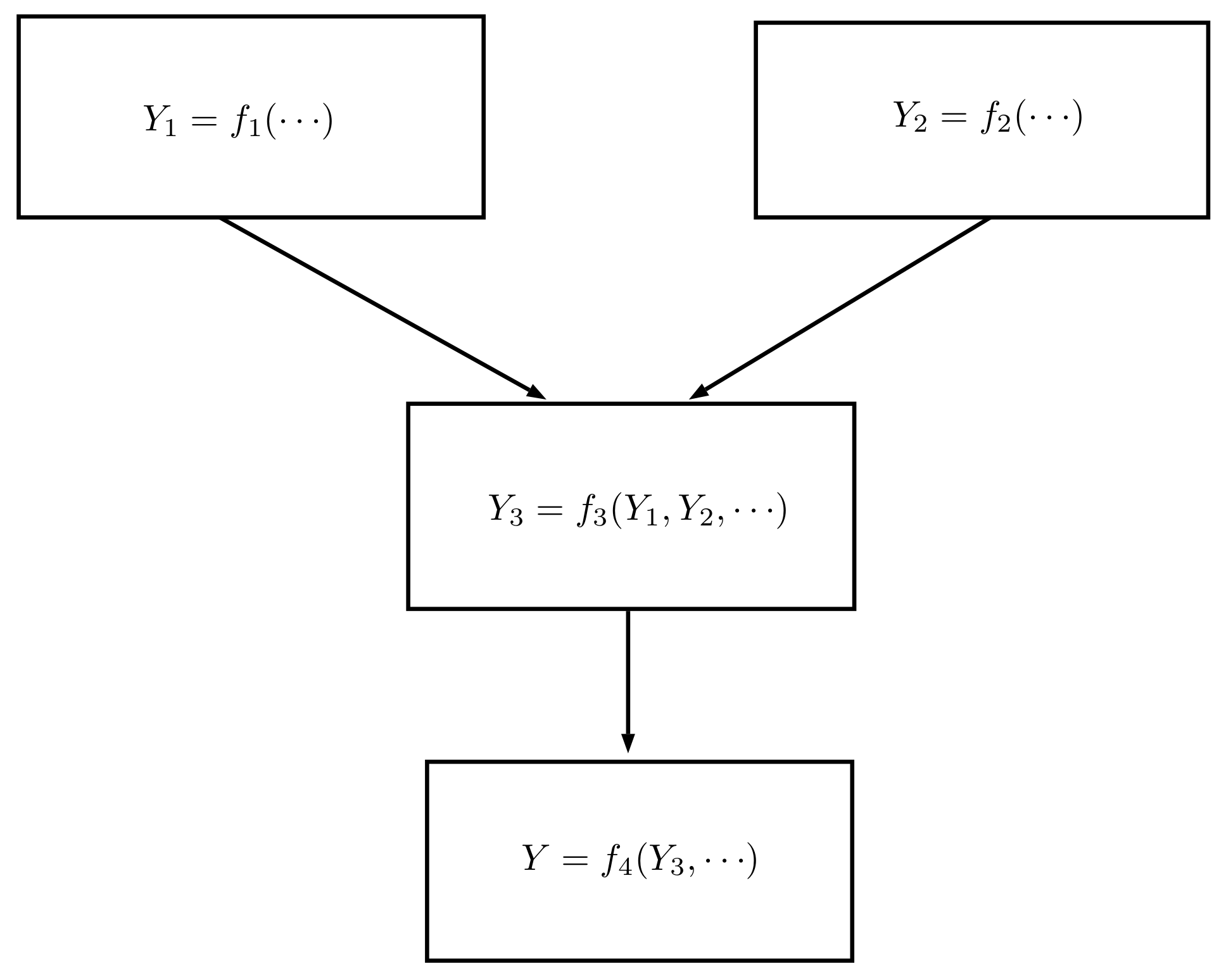
A mathematical expression may often be decomposed into stages and evaluated algorithmically as a sequence of basic operations. For instance, the following is the case:

$$V=v(1-E_{\mathrm{rel}})-E_{\mathrm{off}}-E_{\mathrm{rnd}}$$

and can be broken into four stages (also shown in Figure 1):

$$\begin{array}{cc}\hfill y_1& =1-E_{\mathrm{rel}}\hfill \\ \hfill y_2& =v\times y_1\hfill \\ \hfill y_3& =y_2-E_{\mathrm{off}}\hfill \\ \hfill V=y_4& =y_3-E_{\mathrm{rnd}}.\hfill \end{array}$$

This approach can be applied to measurement models. The evaluation of some arbitrary function $f(x_1,\cdots x_l)$ can be decomposed into $h=1,\cdots ,m$ stages, each producing an intermediate result:

$$y_h=f_h\left({\mathsf{\Lambda }}_h\right),$$

(6)

with the final stage yielding the result $y=y_m$. The set of inputs to the hth stage function, denoted here as ${\mathsf{\Lambda }}_h$, may include previous stage results $y_1,\cdots ,y_{h-1}$ and model inputs $x_1,\cdots x_l$. Using the chain rule for partial differentiation, the components of uncertainty defined in Equation (4) can be evaluated at each stage. The component of uncertainty in $y_h$ due to uncertainty in the jth model input is as follows.

$$u_j\left(y_h\right)=\sum _{z_k\in {\mathsf{\Lambda }}_h}\frac{\partial f_h}{\partial z_k}{u}_j\left(z_k\right).$$

(7)

Thus, the set of components of uncertainty $\{u_1\left(y_h\right),u_2\left(y_h\right),\cdots ,u_l\left(y_h\right)\}$, corresponding to $\{x_1,x_2,\cdots ,x_l\}$, can be evaluated stage-by-stage to finally obtain the set of components of uncertainty in the result, $\{u_1\left(y\right),u_2\left(y\right),\cdots ,u_l\left(y\right)\}$ (when $j=k$, the notation $u_j\left(z_j\right)$ may be simplified to $u\left(z_j\right)$, which is the standard uncertainty of model input $x_j$).

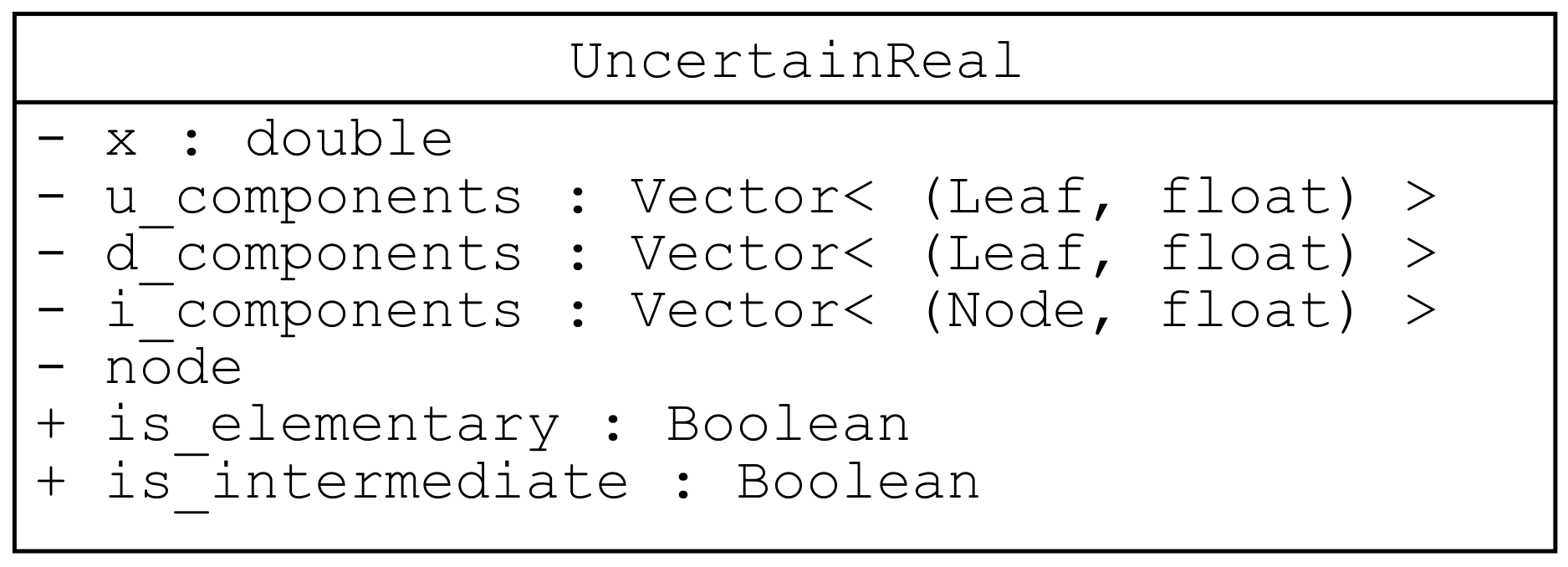
In GTC, an uncertain number is used to encapsulate results at each stage ($y_h$, and the associated components of uncertainty, $\{u_1\left(y_h\right),u_2\left(y_h\right),\cdots \}$). Uncertain numbers provide a convenient and succinct representation for quantities. Their algebraic properties essentially match those of ordinary number types. Thus, data processing algorithms can be expressed with familiar mathematical operations applied to uncertain-number terms representing quantities in a model. There is no need to derive the expressions for components of uncertainty; this is handled algorithmically.

The results of uncertain-number calculations are also transferable: the result of one calculation may be used as an argument in further calculations (as is performed routinely in numerical calculation). This is an open-ended process that can, in principle, continue indefinitely. The transferability of results is needed to support metrological traceability in staged measurement models. This will be discussed further in the next section and in Section 3.6. The open-ended nature of uncertain-number computations is also illustrated in the example shown in Section 2.4.

2.3. Traceability Chains and Uncertainty

Traceability provides accurate and reliable information about physical quantities that can be used to inform decisions. Because a quantity of interest can never be determined exactly, a decision based on the information available may not be correct; there will be some uncertainty—in a colloquial sense—about the correctness of a decision informed by data subject to measurement error. However, the risks associated with poor decision outcomes can be managed if the unpredictability of measurement results can be described in probabilistic terms (i.e., if the accuracy can be quantified). In this sense, the metrologist’s use of the term measurement uncertainty is associated with a likely magnitude of measurement error. To address the need for results that can be relied upon, metrological traceability requires the careful evaluation of measurement uncertainty.

Traceable measurement can be thought of as a collaborative process that is carried out in stages. Ultimately, a traceable measurement is of benefit to a nominal ‘end user’ at the last stage of a traceability chain, who needs information about a quantity to inform a decision (e.g., measuring the weights of shipping containers to inform the loading distribution of a container ship). The accuracy of a final result depends on all the stages; thus, the sources of uncertainty must be traced as far back as the units of measurement realised at the beginning of the process. This ensures that the result is meaningful and comparable with other traceable measurements of the same quantity.

While the GUM’s expression of a measurement model takes the form of a single all-encompassing Equation (1), the staged formulation in Section 2.2 handles the fact that people involved at one stage generally do not have detailed knowledge about processes carried out at other stages. For example, Figure 2 shows a traceable measurement in four parts (e.g., stages 1 and 2 correspond to the realisation of reference standards, stage 3 to the calibration of a measuring instrument using those standards, and stage 4 to an end-user measurement using the calibrated instrument). The staged model is described as follows;

$$\begin{array}{cc}\hfill Y_1& =f_1(\cdots )\hfill \\ \hfill Y_2& =f_2(\cdots )\hfill \\ \hfill Y_3& =f_3(Y_1,Y_2,\cdots )\hfill \\ \hfill Y_4& =f_4(Y_3,\cdots )\hfill \end{array}$$

where unspecified arguments ‘⋯’ represent some subset of the influence quantities $X_1,X_2,\cdots ,X_l$. The end user can probably only formulate a model for stage 4, $f_4(Y_3,\cdots )$; thus, information about earlier stages must be summarised and reported down the chain in a suitable format. If the model was expressed as a single function, the composition of the stages would provide the following.

$$f(X_1,X_2,\cdots ,X_l)=f_4(f_3(f_1(\cdots ),f_2(\cdots ),\cdots ),\cdots ).$$

Now, the outcome of data processing should not be affected by the expression of the model as a single function or a series of functions. This has a bearing on how information should be communicated along a traceability chain [10]. By reporting uncertain numbers between stages, final results can be obtained that are the same as would be found for a single model. Uncertain numbers realise the GUM’s ideal method for evaluating and expressing the uncertainty of a result [3] [Section 0.4].

2.4. A Simple Example

This section presents an example of uncertain-number data processing applied to a simple electrical network. Figure 3 shows an electrical network with three resistors in series. A voltmeter can be connected between the lower terminal and any of the three terminals above, allowing the potential difference between terminals 0 and 1, 0 and 2, or 0 and 3 to be measured ($V_{10}$, $V_{20}$, or $V_{30}$, respectively).

We adopt a simple model for an imperfect voltmeter. The model has three sources of error (influence quantities) that affect the response of a meter (reading) to an input voltage V. A random error (noise), represented as $E_{\mathrm{rnd}}$, affects every reading; a systematic error, $E_{\mathrm{off}}$, contributes a fixed offset to every reading; a systematic relative error, $E_{\mathrm{rel}}$, contributes an error proportional to the reading itself (representing imperfect scaling or non-linearity of the instrument). The relationship between the input voltage, V, and a voltmeter reading, v, is expressed by the model (already shown in Section 2.2).

$$V=v(1-E_{\mathrm{rel}})-E_{\mathrm{off}}-E_{\mathrm{rnd}}.$$

(8)

The influence quantities $E_{\mathrm{rel}}$, $E_{\mathrm{off}}$, and $E_{\mathrm{rnd}}$ are unknown, and so their effects cannot be corrected. However, the displayed value v is used as an approximation for V, because we assume that the instrument is properly adjusted. This is the same as assuming that the residual errors are small enough to be considered approximately zero. The uncertainty in the value of v, due to the estimates $e_{\mathrm{rel}}=e_{\mathrm{off}}=e_{\mathrm{rnd}}=0$, can be found if the uncertainties $u\left(e_{\mathrm{rel}}\right)$, $u\left(e_{\mathrm{off}}\right)$, and $u\left(e_{\mathrm{rnd}}\right)$ are known.

For uncertain number objects representing inputs to a measurement model, we find it helpful to adopt the term elementary uncertain number. Elementary uncertain numbers represent influence quantities. Numeric data must be provided when defining elementary uncertain numbers during the problem initialisation phase; this includes the following: a value (the estimate), a standard uncertainty, and a number of degrees of freedom.

We can use GTC to evaluate properties of the circuit, given measured values and some information about the voltmeter’s characteristics. Objects of the class Voltmeter, shown below, are used for data processing. During initialisation of a new Voltmeter (execution of __init__()), elementary uncertain numbers representing the two systematic errors are created and stored as instance variables (ureal() creates the uncertain numbers).

The applied_voltage() method implements the model Equation (8). It returns an uncertain number for the applied voltage corresponding to a displayed value, v (the second argument, index, is used to create a label for the elementary uncertain number, E_rnd, which is associated with random noise). In the code below, the uncertain numbers V_10, V_20 and V_30 are obtained from measurements of $V_{10}$, $V_{20}$, and $V_{30}$.

We can infer circuit properties from these uncertain-number results. For example, the code below shows how accurately the voltage $V_{10}$ was measured and the most important contributions to the uncertainty in that measured value.

The function display() prints the measured value and a standard uncertainty in parentheses, followed by a list of components of uncertainty in order of magnitude. The label for each component is shown on the left and the magnitude of the component of uncertainty on the right. The two most significant figures of standard uncertainty are shown. Here, $V_{10}$ has a measured value of 0.1258 volts and a standard uncertainty of 0.0050 volts.

Note that the dominant component of uncertainty is associated with the approximation made for systematic offset error $E_{\mathrm{off}}$. Very similar results are obtained for $V_{20}$ and $V_{30}$.

Other circuit properties can be calculated too. For example, the potential difference across resistor 2 can be found by taking the difference between V_20 and V_10. Subtracting those uncertain numbers in the argument, display(V_20-V_10,"V_20-V_10") yields the following.

This is an interesting result, which illustrates the detailed underlying calculation of uncertainty that is performed automatically. The standard uncertainty in the difference here is only $0.00025$ V—significantly less than the standard uncertainty in the individual measurements (both $0.0050$ V). The uncertainty in this voltage difference is lower because it is insensitive to the offset $E_{\mathrm{off}}$ (the offset is exactly the same in both readings). The display of components of uncertainty shows that the sensitivity to $E_{\mathrm{off}}$ has been reduced to zero and that the influence of $E_{\mathrm{rel}}$ is now dominant. We might also expect a smaller contribution to uncertainty to come from relative systematic error $E_{\mathrm{rel}}$. However, that component varies in proportion to the applied voltage (it is a systematic relative error), and since $v_{20}$ is about three times larger than $v_{10}$, the contribution to uncertainty from $E_{\mathrm{rel}}$ is still about two times larger than it was in the direct measurement of $V_{10}$.

3. Aspects of GTC Design

Using the mathematics described in the previous section applied to a given measurement model, GTC is required to evaluate a measured value, a standard uncertainty, and a number of degrees of freedom. This data processing can involve many computational stages and hundreds of influence factors. In addition, GTC can report the components of uncertainty in a result due to the uncertainty of individual influence (input) quantities and the components of uncertainty due to uncertainty in particular intermediate results, as required. Furthermore, it can store and retrieve uncertain numbers, allowing stages along a traceability chain to be appropriately handled.

This section describes how GTC has been designed to meet these challenges. The GTC package was first released four years ago, but our experience with the uncertain-number approach reaches back more than twenty years. We have used different programming languages and changed our thinking about how to implement the technique. For instance, early versions encountered difficulties when the size and variety of the measurement problems grew, and when additional software features were requested. Some programming languages were found to be better suited than others; larger problems exposed scaling weaknesses in our designs; and additional features place strain on some of the data structures and algorithms. GTC implements what we now consider to be our ‘best’ approach.

3.1. Simultaneous Calculation of Value and Uncertainty

Section 2.2 explained that the calculation of components of uncertainty can be handled using the chain rule for partial differentiation when a measurement model is expressed in stages. GTC extends this further by decomposing stage model expressions into very basic operations, such as ×, ÷, sin(), exp(), etc. This is effectively using a computational technique called automatic differentiation [11]. Arithmetic operator overloading and a library of mathematical functions for uncertain numbers are used to automate decomposition of mathematical expressions into simple steps and then to evaluate the value and components of uncertainty at each step.

All the basic uncertain-number functions and arithmetic operations defined in GTC are either univariate or bivariate. For a univariate function, $f_h\left(z\right)$, Equation (7) reduces to the following:

$$u_j\left(y_h\right)=\frac{\partial f_h}{\partial z}{u}_j\left(z\right),$$

(9)

and for a bivariate function, $f_h(z_1,z_2)$, Equation (7) becomes the following.

$$u_j\left(y_h\right)=\frac{\partial f_h}{\partial z_1}{u}_j\left(z_1\right)+\frac{\partial f_h}{\partial z_2}{u}_j\left(z_2\right).$$

(10)

Thus, for example, the uncertain-number trigonometric sine function can be handled as follows. If the value of an uncertain-number input is z, then the value of the uncertain-number result is $y_h=sin\left(z\right)$. Furthermore, if there are two components of uncertainty associated with the input, $u_1\left(z\right)$ and $u_2\left(z\right)$, then the two corresponding components of uncertainty associated with the result are $u_1\left(y_h\right)=c{u}_1\left(z\right)\mathrm{and}{u}_2\left(y_h\right)=c{u}_2\left(z\right)$, where $c=\partial f_h/\partial z=cos\left(z\right)$ is the derivative in (9).

3.2. Unique Identifiers

GTC algorithms track the identity of elementary uncertain numbers representing influence factors. The subscript i that appears on the terms for components of uncertainty, $u_i\left(y\right)$, is the same as the subscript appearing on the influence quantities, $X_i$, in model Equation (1).

$$Y=f(X_1,X_2,\dots ).$$

Software and digital records must somehow keep track of these i’s, even when measurements are carried out in stages, at different locations and at different times. GTC uses a simple tuple of integers as an identifier format. The first integer is kept fixed for a given session while the second integer takes the value of a counter that is incremented each time an elementary uncertain number is created. To ensure that these identifiers are unique in time and space, the first integer is a Universally Unique Identifier (UUID) formatted as a 128-bit integer.

This identifier format reveals nothing about the influence quantity, although identifiers can be arranged in order, which improves the performance of some algorithms. Would a more sophisticated type of identifier be useful? For the purposes of data processing, the only requirement is uniqueness. Nevertheless, GTC already allows text labels to be associated with nodes (used as labels for influence quantities in uncertainty budgets) and a planned enhancement to GTC will allow information about influence quantities to be held in a manifest and indexed by unique identifiers. Such a manifest could accompany a digital record of uncertain-number data. This could address any need for additional metadata about influence quantities, without the burden of minting and configuring more specialised digital objects designed to access information on the internet [12].

3.3. Node Classes

During a GTC calculation, most of the uncertain numbers that are created may be regarded as temporary objects and can be garbage-collected almost immediately. If this is not performed in large problems, the demands on memory can seriously limit performance. To address this, GTC only holds essential information about influence quantities, and information about certain intermediate results as required. This essential information is kept in small node objects, allowing the memory occupied by larger uncertain-number objects to be reclaimed when not required.

There are two classes of node: A Leaf is associated with elementary uncertain numbers and a Node is associated with uncertain numbers representing intermediate results; Leaf is a subclass of Node (Figure 4). A Leaf is created whenever an elementary uncertain number is declared. The information encapsulated includes the following: a value of standard uncertainty; a number of degrees of freedom; a Boolean flag, which identifies objects declared to be independent; a string label, for display purposes; a unique identifier; and two Python collection objects. One of these is the dictionary correlation, which holds values of $r(x_i,x_j)$ for calculations such as Equation (11). The other is the ensemble set, which is used to identify other nodes associated with an ensemble of closely related elementary uncertain numbers. Ensembles are used in the calculation of degrees of freedom described in Section 2.1 (see also Appendix A.1).

While a Leaf is created for every elementary uncertain number, there is no need to create nodes at every stage of a calculation. When intermediate components of uncertainty are required (for an intermediate result of particular significance or when an uncertain number will be stored), the function result() is used to create a new Node (as shown below in Section 3.5 and later in Appendix A.3).

3.4. Propagating Uncertainty

During uncertainty propagation, components of uncertainty must be evaluated at each step. The cumulative effect of these computations can dominate execution time and the demands on memory can be high. Moreover, the overhead of looking up correlation coefficient values for pairs of inputs in Equation (3) during the final calculation of a standard uncertainty is inefficient.

To address this, information about components of uncertainty is stored in several sequences in uncertain-number objects (u_components, d_components and i_components in Figure 5). The elements in these sequences consist of a component of uncertainty paired with a node that holds information about the corresponding influence quantity (see Figure 4).

During calculations, an uncertain number is created at every step. The components of uncertainty are evaluated by weighting the components of uncertainty for the inputs to the step and combining these weighted components when common influences are involved. By keeping the elements in sequences ordered, this process can be handled efficiently by stepping along the sequences and identifying any common influences. The ordering is established by the uid attribute of node objects.

For example, consider the multiplication of a pair of uncertain numbers, $f_h(Z_1,Z_2)=Z_1{Z}_2$. Suppose the component-of-uncertainty sequence for the first argument contains the following elements, where only the first four digits of the UUID integer are shown:

$$\begin{array}{cc}\hfill (7953\dots ,1)& :3,\hfill \\ \hfill (7953\dots ,2)& :-1,\hfill \\ \hfill (7953\dots ,4)& :15,\hfill \\ \hfill (7953\dots ,6)& :-5\hfill \end{array}$$

and the component-of-uncertainty elements for the second argument are as follows.

$$\begin{array}{cc}\hfill (7953\dots ,1)& :-1,\hfill \\ \hfill (7953\dots ,3)& :2,\hfill \\ \hfill (7953\dots ,4)& :2,\hfill \\ \hfill (7953\dots ,5)& :12\hfill \end{array}$$

To obtain the component-of-uncertainty sequence for the product, components in the first sequence are weighted by the value of the second argument and components in the second sequence are weighted by the value of the first argument. The weighted components of common influences are added together (in this case, there is a pair of common influences identified by $(7953\dots ,1)$ and $(7953\dots ,4)$). Thus, if the value of the first argument is 5 and the value of the second is 10, the components of uncertainty for the product are as follows.

$$\begin{array}{cc}\hfill (7953\dots ,1)& :25,\hfill \\ \hfill (7953\dots ,2)& :-10,\hfill \\ \hfill (7953\dots ,3)& :10,\hfill \\ \hfill (7953\dots ,4)& :160,\hfill \\ \hfill (7953\dots ,5)& :60,\hfill \\ \hfill (7953\dots ,6)& :-50\hfill \end{array}$$

When evaluating Equation (3), the number of terms to be summed grows in proportion to the square of the number of input arguments. Moreover, a value of $r(x_i,x_j)$ is needed for every pair of inputs. However, in practice, there are very few non-trivial correlation coefficients assigned (when $i=j$, $r(x_i,x_j)=1$ and usually $r(x_i,x_j)=0$, when $i\ne j$). Therefore, not only is the overhead of looking up correlation coefficients unnecessary but many terms in the double sum are zero. To streamline this calculation, the data for independent and dependent influences are separated in two different component-of-uncertainty sequences (u_components and d_components, in Figure 5). When elementary uncertain numbers are defined, it will be known whether correlation coefficients will be associated with the inputs; thus, dependent and independent influences can be identified and separated. The evaluation of Equation (3) can then be handled more efficiently. For instance, if there are independent estimates $X_1,\cdots ,X_K$ and dependent estimates $X_{K+1},\cdots ,X_l$, the calculation of Equation (3) can be expressed as follows:

$$u\left(y\right)={\left[\sum _{i=1}^K{u}_i^2\left(y\right)+2\sum _{i=K+1}^l\sum _{j=i+1}^l{u}_i\left(y\right)r(x_i,x_j)u_j\left(y\right)\right]}^{1/2},$$

(11)

where the double sum is now only over dependent terms.

3.5. Intermediate Results

In some problems, the interpretation of results is complicated by a large number of influences and, hence, a large number of components of uncertainty. A succinct and often more intuitive presentation can sometimes be obtained, without sacrificing rigour, by reporting the sensitivity of a final result to uncertainty in intermediate results. This is implemented in GTC by using another sequence for components of uncertainty with respect to designated intermediate results (i_components in Figure 5).

To initialise the process of calculating an intermediate component of uncertainty, function result() must be applied to an uncertain number. This seeds a new element in i_components. Thereafter, propagation occurs, as before, by weighting the intermediate components of stage inputs by the partial derivatives of the stage function. The elements in the sequence i_components are also node-value pairs, but a Node rather than a Leaf is used (see Figure 4).

The electrical network example can be used to illustrate the use of intermediate results. Suppose the current through the series network is measured as $1.0000$ mA, with a standard uncertainty of $0.0010$ mA. The resistance of the resistor in the middle of the network, and a breakdown of the contributions to uncertainty in that value, is obtained simply from the following.

The results are as follows.

However, to see how resistance depends on voltage and current measurements, we declare the voltage difference to be an intermediate result and report an uncertainty budget in terms of only the current and voltage.

The results are as follows:

which shows that the contribution to uncertainty from the current measurement is comparable to the contribution from the voltage measured across the resistor. This was not so obvious from the complete list of uncertainty components obtained earlier.

3.6. Storage and Retrieval of Uncertain Numbers

Section 2.3 explained that traceable measurements can be preformed in stages and that, by reporting uncertain numbers when data are processed at each stage, the final uncertainty can be evaluated correctly. The results at one stage will be required at a later time and place. Thus, uncertain numbers must be stored somehow and their identities, which correspond to physical quantities in the actual measurement, must be retained. In GTC, an Archive object is used to manage storage and retrieval of uncertain numbers. The unique identifiers described in Section 3.2 keep track of uncertain-number identities in different Python sessions.

As an example, the code below saves an uncertain number for the voltage difference $V_{20}-V_{10}$ in a text file using a JSON format. Note that the GTC function result() is applied to designate V_20 − V_10 as an intermediate result. This is a prerequisite for storage.

The uncertain number V_20_V_10 for the voltage difference is retrieved by the following:

which produces the following output.

This shows that the necessary information about influence quantities has been retained. Alternatively, the measurements of $V_{10}$ and $V_{20}$ can be saved individually.

Then, in a later session, the difference between the individual results can be evaluated by the following:

which provides exactly the same results.

Although the code here suggests that uncertain-number objects are simply being saved and restored, there is more to it: information about related elementary and intermediate uncertain numbers is also included in the digital record. When an uncertain number is ‘added’ to an archive, objects that hold information about related influences are identified from the component-of-uncertainty sequences. For instance, we showed earlier that the calculation associated with V_10 could be decomposed into stages (Figure 1). Referring again to that figure and thinking about data processing, the error terms, $E_{\mathrm{rel}}$, $E_{\mathrm{off}}$, and $E_{\mathrm{rnd}}$, correspond to elementary uncertain numbers, and each of the circled mathematical operations represents an intermediate stage in the calculation. If the intention is to store the uncertain-number V_10, then information is also required about the voltmeter errors. Figure 6 shows objects with information that would be saved. Later, when the contents of an Archive is loaded back into a different session, this contextual information is immediately restored (nodes are created with the appropriate identifiers). This ensures that when uncertain numbers are retrieved from an archive, they behave as they would have in the context of the original session, which maintains the integrity of information in a traceability chain.

4. Discussion

This paper provides some insight into the usefulness of uncertain numbers, which have the distinctive feature of providing an abstract representation for measured quantities, allowing uncertainty calculations to be automated. Recently, uncertain numbers have been applied to a goniometric measurement system for optical reflectance. The four-axis goniometric system has many configuration errors that must be considered in the measurement model to account for final measurement uncertainties [7]. The application of GTC was carefully compared with alternative computational methods, using Monte Carlo and direct mathematical analysis. GTC was found to be the preferred choice. Using the information provided by uncertain numbers, the authors were able to obtain a better understanding of the measurement system and the inherent correlations between significant measurement errors. This enabled them to significantly improve the accuracy of certain measurements.

The inherent support for metrological traceability is perhaps the most important quality of uncertain numbers. This aspect is implemented in data structures and storage formats used by GTC, which is a particular choice but other formats would be possible. One can easily imagine a more heterogeneous situation, where processing at various stages would be carried out using different software tools. To support this, the format for exchange of data between stages would need to be standardised. That is, there would need to be agreed formats for representing uncertain numbers, which would be used in digital reporting documents such as calibration reports [13].

Digitalisation should offer benefits that are not currently available. The GUM recommends that detailed information about influence quantities be reported at each stage. However, this rarely happens, because calibration certificates and other measurement reports are intended to be read by people; thus, handling the additional data would be difficult. As a consequence, information about common influence factors is rarely shared. A simple situation where this might arise is the scenario of a batch of sensors that are calibrated using a more accurate reference device. If the common reference is ignored, the accuracy of results obtainable from a survey of the sensors’ readings is compromised [14]. However, uncertain-number calibration factors can track common effects and account for them when comparing readings from different sensors. This was illustrated in Section 2.4, where E_off contributed a common offset to single voltage readings but nothing to uncertainty in the voltage difference. It is also worth noting that a ‘smart’ sensor capable of reporting uncertain-number results would not need to process a lot of information. As was the case of the simple voltmeter, a model of the sensor measurement might only require a few influence factors and the calculations would be simple.

The various stages of a traceable measurement often occur in different locations (national metrology institute, second-tier calibration laboratory, etc.) but they may also happen at different times in the same location. For example, a working standard might be calibrated in-house against an externally calibrated transfer standard. The working standard would then be used repeatedly to calibrate different instruments at different times. Importantly, measurement errors realised when at the time the working standard is calibrated should be treated as systematic effects in subsequent instrument calibrations. Performing this would allow any bias, or correlation, in downstream measurement results using those instruments to be accounted for correctly. This could be easily handled by digitalisation if uncertain-number storage and retrieval mechanisms are used to save calibration data for the working standard and later retrieve it for reuse when instruments are calibrated.

During formal international measurement comparisons, national metrology institutes (NMIs) go to much greater pains when reporting measurement data than they do for regular calibration work. These international comparisons assess the competence of NMIs in performing specific types of measurement. The more detailed reporting requirements in comparisons align with the GUM’s recommendations in this case. A recent study, which explored a future scenario where an uncertain-number reporting format was used by all participants, showed that using uncertain numbers would not only provide the information required, but they would also simplify comparison analysis and comparison linking and provide additional insights into the results [6].

Measurement models are needed in order to use uncertain numbers effectively. The close correspondence between quantity terms in a model and uncertain numbers in data processing routines makes software development and testing more robust and reliable and avoids the need to explicitly derive expressions for the components of uncertainty from a model, which GTC handles automatically. However, although modelling lies at the heart of the GUM’s approach, skilled metrologists are often confident in their ability to assess measurement uncertainty heuristically and frequently elide the formal modelling step. This presents a problem for digitalisation, because digital systems need a rigorous formal problem definition for autonomous operation. Some tutorial guidance on developing measurement models has been provided in a recent booklet [15] and is also the subject of another paper [16]. There is also a new supplement to the GUM, which deals with modelling [17].

One common conceptual difficulty when modelling is the omission of influence quantities estimated as zero. These terms would not be needed in conventional data processing; however, they must be modelled, because the actual (unknown) values affect the final measurement result, and so they contribute to uncertainty. Influence quantities with trivial estimates are often called residual errors. The electrical network example, in Section 2.4, included three residual errors that were all estimated as zero. These terms were represented by uncertain numbers and modelled imperfect voltmeter behaviour.

5. Conclusions

GTC is a software tool for data processing with automatic evaluation of measurement uncertainty. It follows international best-practice, described in the GUM, and offers useful extensions to those methods for important special cases. The use of uncertain numbers is a distinctive feature of GTC. The uncertain-number data-type facilitates data processing, which can be performed in a piece-wise and open-ended manner. This allows calculations to be more easily matched to the models of a measurement performed in stages. The automation of uncertainty calculations allows measurement data processing to be made more rigorous, which can lead to accuracy enhancement in some cases. The uncertain-number format significantly exceeds current paper-based practices that support traceability. Therefore, GTC and the data structures used to implement uncertain numbers are a useful example of software that meets the requirements of a fully functional digital infrastructure for metrological traceability.

References

1. Hackel, S.; Härtig, F.; Hornig, J.; Wiedenhöfer, T. The Digital Calibration Certificate. PTB-Mitteilungen 2017, 127, 75–81. [Google Scholar] [CrossRef]
2. Thiel, F. Digital transformation of legal metrology—The European Metrology Cloud. OIML Bull. 2018, 59, 10–21. [Google Scholar]
3. BIPM; IEC; IFCC; ILAC; ISO; IUPAC; IUPAP; OIML. Evaluation of Measurement Data—Guide to the Expression of Uncertainty in Measurement JCGM 100:2008 (GUM 1995 with Minor Corrections), 1st ed.; BIPM Joint Committee for Guides in Metrology: Paris, France, 2008. [Google Scholar]
4. Hall, B.D. Computing with Uncertain Numbers. Metrologia 2006, 43, L56–L61. [Google Scholar] [CrossRef]
5. Hall, B.D.; Borbely, J.S. GUM Tree Calculator and v1.3.6. Available online: https://github.com/MSLNZ/GTC; https://doi.org/10.5281/zenodo.5459479 (accessed on 13 November 2021).
6. Hall, B.D.; Koo, A. Digital Representation of Measurement Uncertainty: A Case Study Linking an RMO Key Comparison with a CIPM Key Comparison. Metrology 2021, 1, 166–181. [Google Scholar] [CrossRef]
7. Molloy, E.; Saunders, P.; Koo, A. Effects of rotation errors on goniometric measurements. Metrologia 2021, in press. [Google Scholar] [CrossRef]
8. Walpole, R.E.; Myers, R.H.; Myers, S.L.; Ye, K. Probability & Statistics for Engineers and Scientists, 8th ed.; Pearson Education: Upper Saddle River, NJ, USA, 2007; p. 07458. [Google Scholar]
9. Willink, R. A generalization of the Welch–Satterthwaite formula for use with correlated uncertainty components. Metrologia 2007, 44, 340. [Google Scholar] [CrossRef]
10. Hall, B.D.; White, D.R. Digital representation of measurement uncertainty for metrological traceability. In Advanced Mathematical and Computational Techniques in Metrology XII; Pavese, F., Forbes, A.B., Chunovkina, A.G., Zhang, N.F., Eds.; Series on Advances in Mathematics for Applied Sciences; World Scientific: Singapore, 2021; Volume 90, pp. 262–272. [Google Scholar]
11. Rall, L.B.; Corliss, G.F. An Introduction to Automatic Differentiation. In Computational Differentiation: Techniques Applications, and Tools; Berz, M., Bischof, C.H., Griewankpp, A., Eds.; Siam Proceedings in Applied Mathematics Series; SIAM: Philadelphia, PA, USA, 1996; Volume 89, pp. 1–17. [Google Scholar]
12. Klump, J.; Huber, R. 20 Years of Persistent Identifiers—Which Systems are Here to Stay? Data Sci. J. 2017, 16, 9. [Google Scholar] [CrossRef]
13. Hackel, S.; Härtig, F.; Hornig, J.; Wiedenhöfer, T. Metrologie für die Digitalisierung von Wirtschaft und Gesellschaft. 2017. Available online: https://oar.ptb.de/files/download/5a9808d94c91840d190b3891 (accessed on 13 November 2021).
14. Hall, B.D. An Opportunity to Enhance the Value of Metrological Traceability in Digital Systems, 2nd ed.; Workshop on Metrology for Industry 4.0 and IoT (MetroInd4.0 IoT); IEEE: Naples, Italy, 2019; pp. 16–21. [Google Scholar]
15. Hall, B.D.; White, D.R. An Introduction to Measurement Uncertainty; Measurement Standards Laboratory of New Zealand: New Zealand, 2020. [Google Scholar] [CrossRef]
16. Hall, B.D. Object-oriented software for evaluating measurement uncertainty. Meas. Sci. Technol. 2013, 24, 055004. [Google Scholar] [CrossRef]
17. BIPM; IEC; ILAC; IFCC; ISO; IUPAC; IUPAP; OIML. Guide to the Expression of Uncertainty in Measurement—Part 6: Developing and Using Measurement Models JCGM GUM-6:2020, 1st ed.; BIPM Joint Committee for Guides in Metrology: Paris, France, 2020. [Google Scholar]
18. Hall, B.D.; Borbely, J.S. GTC Documentation. Available online: https://gtc.readthedocs.io/en/stable/ (accessed on 13 November 2021).
19. Hall, B.D. Evaluating the measurement uncertainty of complex quantities: A selective review. Metrologia 2015, 53, S25–S31. [Google Scholar] [CrossRef]
20. Willink, R.; Hall, B.D. A classical method for uncertainty analysis with multidimensional data. Metrologia 2002, 39, 361–369. [Google Scholar] [CrossRef]
21. Lafarge, T.; Possolo, A. The NIST Uncertainty Machine. Ncsli Meas. J. Meas. Sci. 2015, 10, 20–27. [Google Scholar] [CrossRef]
22. Zeier, M.; Wollensack, M.; Hoffmann, J. METAS UncLib—A measurement uncertainty calculator for advanced problems. Metrologia 2012, 49, 809–815. [Google Scholar] [CrossRef] [Green Version]
23. Wollensack, M.; Hoffmann, J.; Ruefenacht, J.; Zeier, M. VNA Tools II: S-parameter uncertainty calculation. In Proceedings of the 79th ARFTG Microwave Measurement Conference Digest, Montreal, QC, Canada, 22–22 June 2012. [Google Scholar] [CrossRef]
24. Lebigot, E.O. Uncertainties: A Python Package for Calculations with Uncertainties. Available online: http://pythonhosted.org/uncertainties (accessed on 13 November 2021).
25. Bevington, P.R.; Robinson, D.K. Data Reduction and Error Analysis; McGraw-Hill: New York, NY, USA, 2003. [Google Scholar]
Figure 1. Decomposition of V = v ( 1 E rel ) E off E rnd into a sequence of arithmetic operations.
Metrology 02 00009 g001
Figure 2. A measurement carried out in four stages. Arrows indicate the transfer of information about intermediate results. The unspecified function arguments ‘⋯’ represent external quantities that influence the procedures. This figure does not represent a particular measurement, but the four stages may be regarded as follows: realisation of unit reference standards (stages 1 and 2), calibration of an instrument using the standards (stage 3), and a measurement made with the calibrated instrument (stage 4).
Metrology 02 00009 g002
Figure 3. Three resistors in an electrical network. A voltage measurement can be performed between the bottom terminal and any terminal above.
Metrology 02 00009 g003
Figure 4. A UML diagram for node classes. There are two types of node: Node and Leaf. Leaf nodes are associated with elementary uncertain real numbers, while objects of the parent class Node may be associated with intermediate uncertain-number results. The uid attribute can be used to sort nodes. The first integer in uid is a common UUID value for all the nodes created in a Python session, while the second integer enumerates the nodes created in that session.
Metrology 02 00009 g004
Figure 5. A UML class diagram for an uncertain real number. Vector objects contain sequences of pairs (the Node and Leaf classes in Figure 4). The Vectors u_components and d_components hold components of uncertainty for independent and dependent influences, respectively. The Vector i_components holds components of uncertainty with respect to designated intermediate results. The private node attribute will refer to a Leaf when an UncertainReal object is elementary, or to a Node when the object is an intermediate result, but otherwise, the attribute is not assigned.
Metrology 02 00009 g005
Figure 6. A UML object diagram showing information that would be collected when the uncertain number V_10 is stored. The three Leaf objects contain information about the error terms in the voltmeter measurement model: the fixed offset, the relative error and the random noise. Only one Leaf for the influence of noise is shown; however, if several readings had been taken there would be a different node for each reading.
Metrology 02 00009 g006
Publisher’s Note: MDPI stays neutral with regard to jurisdictional claims in published maps and institutional affiliations.