
A Shared Metrological Framework for Trustworthy Virtual Experiments and Digital Twins

 , , , , , ,
  , and
, and
Abstract
1. Introduction
1.1. VEs in the Literature
1.2. DTs in the Literature
- A physical entity, representing the entity the DT models and controls embedded in a physical environment tasked to carry out certain physical process; and
- A virtual entity fit in a virtual environment, i.e., the digital representation of the physical entity and its environment.
1.3. Scope of the Work
2. A Novel and Harmonized Definition of VEs and DTs
2.1. Definition of VEs
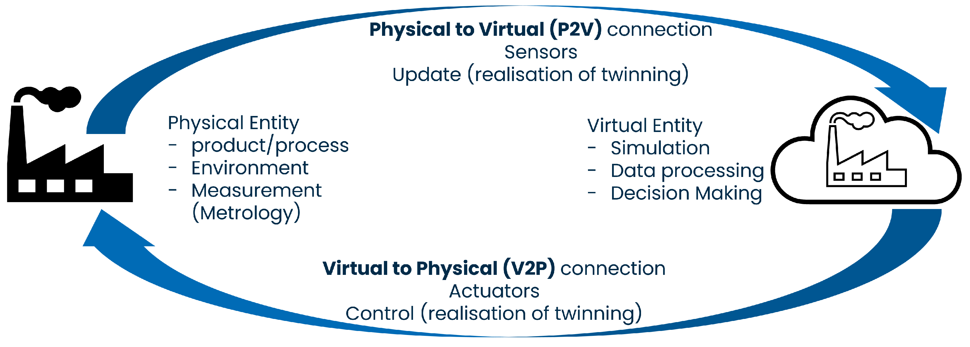
2.2. Definition of DTs
- A physical environment, which embeds the physical entity(ies) to which the DT refers;
- A virtual environment with the virtual entities that models the considered physical asset(s);
- A P2V connection between the physical and virtual environments;
- A V2P connection that implements prevention and control strategies to achieve the target accuracy in the physical system, thus establishing a bi-directional data flow.
2.3. Connection between VEs and DTs
- A DT virtually mimics a real device by processing incoming sensor data in real time and can influence the real device by sending commands to its actuators, also in real time. A VE is conceptually something different. It simulates how measurement data are generated based on a simulated artifact and knowledge of the measurement instrument. However, the virtual entity of a DT can contain a VE, which is then modeling a measuring instrument, for example.
- A VE is especially useful when the relationship between a measurand and measured data is complex and/or indirect. The measurements performed for a DT might be straightforward to interpret by the DT model, or they may be indirect as well. The usefulness of a DT lies in the continuous monitoring and predictive maintenance and correction of physical systems, even when they are easy and simple to model.
- A DT shows the current state of several parts, as transmitted by auxiliary sensors, as well as the the result of the system’s target operation, e.g., the measured quantity for a measuring instrument, the position for a machine tool, or process key performance indicators (KPIs) for a manufacturing system. In a VE, on the contrary, usually, only the final measurement data are used. Therefore, the vector of measured data X is much longer for a DT.
- A DT must involve a dynamic, time-dependent, state-space model. A VE, on the other hand, assumes that the model does not change over time. It models either the current state of a measuring instrument (in case of a direct measurement) or the complete dataset that resulted from the entire measurement (in case of an indirect measurement). If the settings change, a new VE needs to be performed. Hence, a VE can be the “inner part” of a DT, which models the whole (time-dependent) process.
3. Uncertainty Evaluation for VEs and DTs
3.1. Uncertainty Evaluation Involving VEs
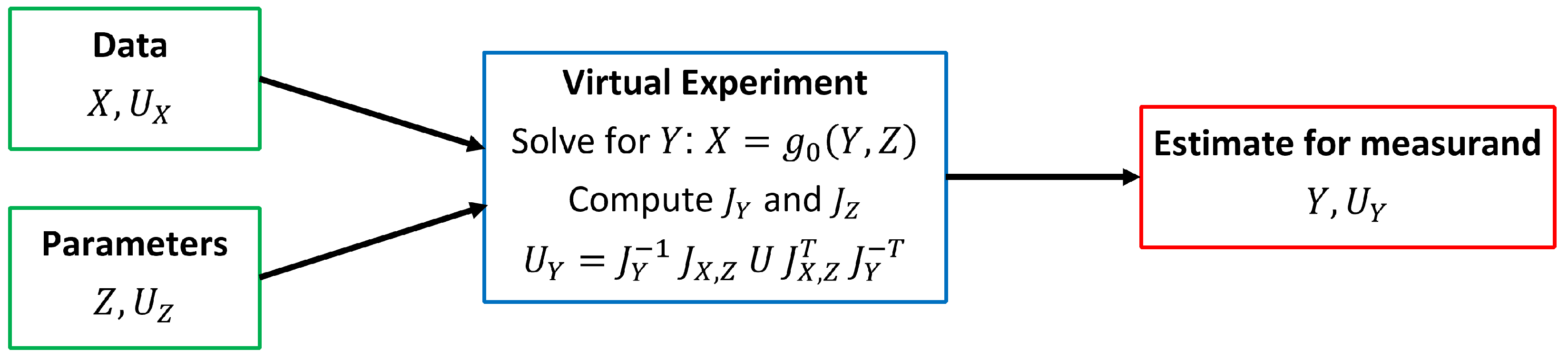
3.1.1. LPU-via-VE
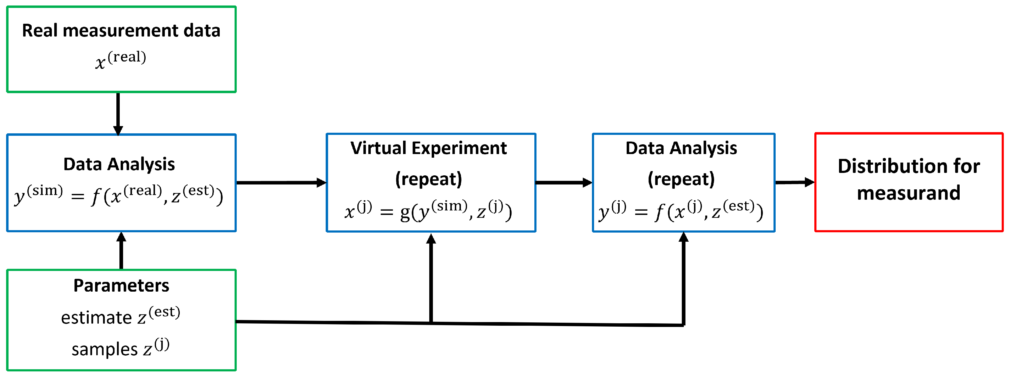
3.1.2. PoD-via-VE
3.2. Uncertainty Evaluation for DTs
- Uncertainty of the diagnosis, i.e., errors and uncertainties related to the sensors devoted to measuring the current state of the system;
- Uncertainty of the prognosis, i.e., errors and uncertainties related to the simulative model (e.g, VE) embedded in the virtual asset;
- Epistemic errors, i.e., errors to modeling strategy, which by extension include the fidelity and the twinning rate.
- How to establish traceability for a DT;
- How to define the uncertainty and accuracy of the P2V model;
- How to include the V2P correction and related uncertainty in the physical measurement of metrological characteristics and uncertainty.
3.2.1. Problem Statement
3.2.2. Establishing Traceability for a DT
- Calibrating the sensors with traceable material standards;
- Calibrating the model response by means of a comparison with traceable measurements with associated lower uncertainty and better accuracy; and
- Calibrating the actuators.
3.2.3. Definition of Uncertainty and Accuracy of the P2V Model
- The traceability of the sensors (coming from calibration certificates);
- The task-based influence factors to the measurement uncertainty of the sensors (i.e., the reproducibility, resolution);
- The model metrological performances (i.e., accuracy and precision); and
- Environmental conditions.
3.2.4. Effect of Closed-Loop Feedback Control on Measurement Uncertainty
3.3. Challenges
4. Applications
4.1. VE of a CMM
4.1.1. Description of the Application
4.1.2. LPU-via-VE
4.1.3. PoD-via-VE
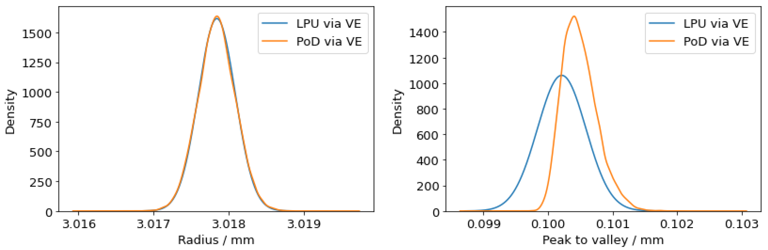
4.1.4. Numerical Results
4.2. DT of a Cobot
5. Conclusions
- The two definitions clearly distinguish between static VEs and time-varying DTs;
- The definitions are harmonized, allowing for using an VE as a core part (digital model) within a DT, for example, by means of a common mathematical framework; and
- The definitions allow for considering uncertainties constituting a basis for trustworthy and traceable VEs and DTs.
Author Contributions
Funding
Data Availability Statement
Conflicts of Interest
References
- Jones, D.; Snider, C.; Nassehi, A.; Yon, J.; Hicks, B. Characterising the Digital Twin: A systematic literature review. CIRP J. Manuf. Sci. Technol. 2020, 29, 36–52. [Google Scholar] [CrossRef]
- Flegr, S.; Kuhn, J.; Scheiter, K. When the whole is greater than the sum of its parts: Combining real and virtual experiments in science education. Comput. Educ. 2023, 197, 104745. [Google Scholar] [CrossRef]
- Chinesta, F.; Cueto, E.; Abisset-Chavanne, E.; Duval, J.L.; Khaldi, F.E. Virtual, Digital and Hybrid Twins: A New Paradigm in Data-Based Engineering and Engineered Data. Arch. Comput. Methods Eng. 2020, 27, 105–134. [Google Scholar] [CrossRef]
- Kennedy, M.C.; O’Hagan, A. Bayesian Calibration of Computer Models. J. R. Stat. Soc. Ser. B Stat. Methodol. 2001, 63, 425–464. [Google Scholar] [CrossRef]
- Bayarri, M.; Berger, J.; Cafeo, J.; Garcia-Donato, G.; Liu, F.; Palomo, J.; Parthasarathy, R.; Paulo, R.; Sacks, J.; Walsh, D. Computer model validation with functional output. Ann. Stat. 2007, 35, 1874–1906. [Google Scholar] [CrossRef]
- Fuller, A.; Fan, Z.; Day, C.; Barlow, C. Digital Twin: Enabling Technologies, Challenges and Open Research. IEEE Access 2020, 8, 108952–108971. [Google Scholar] [CrossRef]
- Wright, L.; Davidson, S. How to tell the difference between a model and a digital twin. Adv. Model. Simul. Eng. Sci 2020, 7, 13. [Google Scholar] [CrossRef]
- Wübbeler, G.; Marschall, M.; Kniel, K.; Heißelmann, D.; Härtig, F.; Elster, C. GUM-Compliant Uncertainty Evaluation Using Virtual Experiments. Metrology 2022, 2, 114–127. [Google Scholar] [CrossRef]
- Hughes, F.; Marschall, M.; Wübbeler, G.; Kok, G.; van Dijk, M.; Elster, C. JCGM 101-compliant uncertainty evaluation using virtual experiments. arXiv 2024, arXiv:2404.10530. [Google Scholar]
- Scholz, G.; Fortmeier, I.; Marschall, M.; Stavridis, M.; Schulz, M.; Elster, C. Experimental Design for Virtual Experiments in Tilted-Wave Interferometry. Metrology 2022, 2, 84–97. [Google Scholar] [CrossRef]
- Jing, X.; Wang, C.; Pu, G.; Xu, B.; Zhu, S.; Dong, S. Evaluation of measurement uncertainties of virtual instruments. Int. J. Adv. Manuf. Technol. 2005, 27, 1202–1210. [Google Scholar] [CrossRef]
- Kok, G.; Wübbeler, G.; Elster, C. Impact of Imperfect Artefacts and the Modus Operandi on Uncertainty Quantification Using Virtual Instruments. Metrology 2022, 2, 311–319. [Google Scholar] [CrossRef]
- Heißelmann, D.; Franke, M.; Rost, K.; Wendt, K.; Kistner, T.; Schwehn, C. Determination of measurement uncertainty by Monte Carlo simulation. In Advanced Mathematical and Computational Tools in Metrology and Testing XI; World Scientific: Singapore, 2018; pp. 192–202. [Google Scholar] [CrossRef]
- Straka, M.; Weissenbrunner, A.; Koglin, C.; Höhne, C.; Schmelter, S. Simulation Uncertainty for a Virtual Ultrasonic Flow Meter. Metrology 2022, 2, 335–359. [Google Scholar] [CrossRef]
- Weissenbrunner, A.; Ekat, A.K.; Straka, M.; Schmelter, S. A virtual flow meter downstream of various elbow configurations. Metrologia 2023, 60, 054002. [Google Scholar] [CrossRef]
- Grieves, M. Digital twin: Manufacturing excellence through virtual factory replication. White Pap. 2014, 1, 1–7. [Google Scholar]
- Grieves, M.; Vickers, J. Digital Twin: Mitigating Unpredictable, Undesirable Emergent Behavior in Complex Systems. In Transdisciplinary Perspectives on Complex Systems: New Findings and Approaches; Kahlen, F.J., Flumerfelt, S., Alves, A., Eds.; Springer International Publishing: Cham, Switzerland, 2017; pp. 85–113. [Google Scholar] [CrossRef]
- Errandonea, I.; Beltrán, S.; Arrizabalaga, S. Digital Twin for maintenance: A literature review. Comput. Ind. 2020, 123, 103316. [Google Scholar] [CrossRef]
- Yoon, S.; Koo, J. In situ model fusion for building digital twinning. Build. Environ. 2023, 243, 110652. [Google Scholar] [CrossRef]
- Zhang, C.; Sun, Q.; Sun, W.; Shi, Z.; Mu, X. Performance-oriented digital twin assembly of high-end equipment: A review. Int. J. Adv. Manuf. Technol. 2023, 126, 4723–4748. [Google Scholar] [CrossRef]
- Liu, L.; Zhang, X.; Wan, X.; Zhou, S.; Gao, Z. Digital twin-driven surface roughness prediction and process parameter adaptive optimization. Adv. Eng. Inform. 2022, 51, 101470. [Google Scholar] [CrossRef]
- Cimino, C.; Negri, E.; Fumagalli, L. Review of digital twin applications in manufacturing. Comput. Ind. 2019, 113, 103130. [Google Scholar] [CrossRef]
- Pang, J.; Zheng, P.; Li, S.; Liu, S. A verification-oriented and part-focused assembly monitoring system based on multi-layered digital twin. J. Manuf. Syst. 2023, 68, 477–492. [Google Scholar] [CrossRef]
- Verna, E.; Puttero, S.; Genta, G.; Galetto, M. Toward a concept of digital twin for monitoring assembly and disassembly processes. Qual. Eng. 2024, 36, 453–470. [Google Scholar] [CrossRef]
- Magnanini, M.C.; Tolio, T.A. A model-based Digital Twin to support responsive manufacturing systems. CIRP Ann. 2021, 70, 353–356. [Google Scholar] [CrossRef]
- Mengke Sun, Z.C.; Zhao, N. Design of intelligent manufacturing system based on digital twin for smart shop floors. Int. J. Comput. Integr. Manuf. 2023, 36, 542–566. [Google Scholar] [CrossRef]
- Kononowicz, A.A.; Woodham, L.A.; Edelbring, S.; Stathakarou, N.; Davies, D.; Saxena, N.; Car, L.T.; Carlstedt-Duke, J.; Car, J.; Zary, N. Virtual Patient Simulations in Health Professions Education: Systematic Review and Meta-Analysis by the Digital Health Education Collaboration. J. Med. Internet Res. 2019, 21, e14676. [Google Scholar] [CrossRef] [PubMed]
- Cellina, M.; Cè, M.; Alì, M.; Irmici, G.; Ibba, S.; Caloro, E.; Fazzini, D.; Oliva, G.; Papa, S. Digital Twins: The New Frontier for Personalized Medicine? Appl. Sci. 2023, 13, 7940. [Google Scholar] [CrossRef]
- Kasper, L.; Birkelbach, F.; Schwarzmayr, P.; Steindl, G.; Ramsauer, D.; Hofmann, R. Toward a Practical Digital Twin Platform Tailored to the Requirements of Industrial Energy Systems. Appl. Sci. 2022, 12, 6981. [Google Scholar] [CrossRef]
- Fathy, Y.; Jaber, M.; Nadeem, Z. Digital twin-driven decision making and planning for energy consumption. J. Sens. Actuator Netw. 2021, 10, 37. [Google Scholar] [CrossRef]
- Ghenai, C.; Husein, L.A.; Al Nahlawi, M.; Hamid, A.K.; Bettayeb, M. Recent trends of digital twin technologies in the energy sector: A comprehensive review. Sustain. Energy Technol. Assess. 2022, 54, 102837. [Google Scholar] [CrossRef]
- Deng, T.; Zhang, K.; Shen, Z.J.M. A systematic review of a digital twin city: A new pattern of urban governance toward smart cities. J. Manag. Sci. Eng. 2021, 6, 125–134. [Google Scholar] [CrossRef]
- Dani, A.A.H.; Supangkat, S.H.; Lubis, F.F.; Nugraha, I.G.B.B.; Kinanda, R.; Rizkia, I. Development of a Smart City Platform Based on Digital Twin Technology for Monitoring and Supporting Decision-Making. Sustainability 2023, 15, 14002. [Google Scholar] [CrossRef]
- Boschert, S.; Rosen, R. Digital Twin—The Simulation Aspect. In Mechatronic Futures: Challenges and Solutions for Mechatronic Systems and Their Designers; Hehenberger, P., Bradley, D., Eds.; Springer International Publishing: Cham, Switzerland, 2016; pp. 59–74. [Google Scholar] [CrossRef]
- Schleich, B.; Anwer, N.; Mathieu, L.; Wartzack, S. Shaping the digital twin for design and production engineering. CIRP Ann. 2017, 66, 141–144. [Google Scholar] [CrossRef]
- Liu, M.; Fang, S.; Dong, H.; Xu, C. Review of digital twin about concepts, technologies, and industrial applications. J. Manuf. Syst. 2021, 58, 346–361. [Google Scholar] [CrossRef]
- VanDerHorn, E.; Mahadevan, S. Digital Twin: Generalization, characterization and implementation. Decis. Support Syst. 2021, 145, 113524. [Google Scholar] [CrossRef]
- ISO 23247-1:2021; Automation Systems and Integration—Digital Twin Framework for Manufacturing. Part 1: Overview and General Principles. International Organization for Standardization: Geneva, Switzerland, 2021.
- ISO/IEC 30173:2023; Digital Twin—Concepts and Terminology. International Organization for Standardization and International Electrotechnical Commission: Geneva, Switzerland, 2023.
- Tang, W.; Xu, G.; Zhang, S.; Jin, S.; Wang, R. Digital Twin-Driven Mating Performance Analysis for Precision Spool Valve. Machines 2021, 9, 157. [Google Scholar] [CrossRef]
- Zhao, Z.; Wang, S.; Wang, Z.; Wang, S.; Ma, C.; Yang, B. Surface roughness stabilization method based on digital twin-driven machining parameters self-adaption adjustment: A case study in five-axis machining. Int. J. Comput. Integr. Manuf. 2022, 33, 943–952. [Google Scholar] [CrossRef]
- Modoni, G.E.; Stampone, B.; Trotta, G. Application of the Digital Twin for in process monitoring of the micro injection moulding process quality. Comput. Ind. 2022, 135, 103568. [Google Scholar] [CrossRef]
- Xin, Y.; Chen, Y.; Li, W.; Li, X.; Wu, F. Refined Simulation Method for Computer-Aided Process Planning Based on Digital Twin Technology. Micromachines 2022, 13, 620. [Google Scholar] [CrossRef] [PubMed]
- De Ketelaere, B.; Smeets, B.; Verboven, P.; Nicolaï, B.; Saeys, W. Digital twins in quality engineering. Qual. Eng. 2022, 34, 404–408. [Google Scholar] [CrossRef]
- Guo, Y.; Klink, A.; Bartolo, P.; Guo, W.G. Digital twins for electro-physical, chemical, and photonic processes. CIRP Ann. 2023, 72, 593–619. [Google Scholar] [CrossRef]
- Franciosa, P.; Sokolov, M.; Sinha, S.; Sun, T.; Ceglarek, D. Deep learning enhanced digital twin for Closed-Loop In-Process quality improvement. CIRP Ann. 2020, 69, 369–372. [Google Scholar] [CrossRef]
- Bergs, T.; Biermann, D.; Erkorkmaz, K.; M’Saoubi, R. Digital twins for cutting processes. CIRP Ann. 2023, 72, 541–567. [Google Scholar] [CrossRef]
- Karve, P.M.; Guo, Y.; Kapusuzoglu, B.; Mahadevan, S.; Haile, M.A. Digital twin approach for damage-tolerant mission planning under uncertainty. Eng. Fract. Mech. 2020, 225, 106766. [Google Scholar] [CrossRef]
- Wright, L.; Davidson, S. Digital twins for metrology; metrology for digital twins. Meas. Sci. Technol. 2024, 35, 051001. [Google Scholar] [CrossRef]
- Zheng, Y.; Wang, S.; Li, Q.; Li, B. Fringe projection profilometry by conducting deep learning from its digital twin. Opt. Express 2020, 28 24, 36568–36583. [Google Scholar] [CrossRef]
- Poroskun, I.; Rothleitner, C.; Heißelmann, D. Structure of digital metrological twins as software for uncertainty estimation. J. Sensors Sens. Syst. 2022, 11, 75–82. [Google Scholar] [CrossRef]
- Härtig, F.; Kniel, K.; Heißelmann, D. Das Virtuelle Koordinatenmessgerät—ein Digitaler Metrologischer Zwilling. TM-Tech. Mess. 2023, 90, 548–556. [Google Scholar] [CrossRef]
- Shao, G.; Hightower, J.; Schindel, W. Credibility consideration for digital twins in manufacturing. Manuf. Lett. 2023, 35, 24–28. [Google Scholar] [CrossRef]
- Trustworthy Virtual Experiments and Digital Twins—ViDiT. Available online: https://www.vidit.ptb.de (accessed on 13 March 2024).
- BIPM; IEC; IFCC; ILAC; ISO; IUPAC; IUPAP; OIML. Evaluation of Measurement Data—Guide to the Expression of Uncertainty in Measurement; JCGM 100:2008; Joint Committee for Guides in Metrology: Sèvres, France, 2008. [Google Scholar]
- BIPM; IEC; IFCC; ILAC; ISO; IUPAC; IUPAP; OIML. Evaluation of Measurement Data—Supplement 1 to the “Guide to the Expression of Uncertainty in Measurement”—Propagation of Distributions Using a Monte Carlo Method; JCGM 101:2008; Joint Committee for Guides in Metrology: Sèvres, France, 2008. [Google Scholar]
- BIPM; IEC; IFCC; ILAC; ISO; IUPAC; IUPAP; OIML. Evaluation of Measurement Data—Supplement 2 to the “Guide to the Expression of Uncertainty in Measurement”—Extension to any Number of Output Quantities; JCGM 102:2011; Joint Committee for Guides in Metrology: Sèvres, France, 2011. [Google Scholar]
- Elster, C. Bayesian uncertainty analysis compared with the application of the GUM and its supplements. Metrologia 2014, 51, S159. [Google Scholar] [CrossRef]
- van Dijk, M.; Kok, G. Comparison of uncertainty evaluation methods for virtual experiments with an applciation to a virtual CMM. In Proceedings of the IMEKO XXIV World Congress, Hamburg, Germany, 26–29 August 2024. [Google Scholar]
- Kok, G.; van Dijk, M.; Wübbeler, G.; Elster, C. Virtual experiments for the assessment of data analysis and uncertainty quantification methods in scatterometry. Metrologia 2023, 60, 044001. [Google Scholar] [CrossRef]
- Marschall, M.; Fortmeier, I.; Stavridis, M.; Hughes, F.; Elster, C. Bayesian uncertainty evaluation applied to the tilted-wave interferometer. Opt. Express 2024, 32, 18664–18683. [Google Scholar] [CrossRef]
- Possolo, A.; Toman, B. Assessment of measurement uncertainty via observation equations. Metrologia 2007, 44, 464–475. [Google Scholar] [CrossRef]
- Verna, E.; Genta, G.; Galetto, M.; Franceschini, F. Zero defect manufacturing: A self-adaptive defect prediction model based on assembly complexity. Int. J. Comput. Integr. Manuf. 2023, 36, 155–168. [Google Scholar] [CrossRef]
- Wu, T.; Yang, F.; Farooq, U.; Li, X.; Jiang, J. An online learning method for constructing self-update digital twin model of power transformer temperature prediction. Appl. Therm. Eng. 2024, 237, 121728. [Google Scholar] [CrossRef]
- Grieves, M.W. Digital Twins: Past, Present, and Future. In The Digital Twin; Crespi, N., Drobot, A.T., Minerva, R., Eds.; Springer International Publishing: Cham, Switzerland, 2023; pp. 97–121. [Google Scholar] [CrossRef]
- Gelman, A.; Carlin, J.B.; Stern, H.S.; Rubin, D.B. Bayesian Data Analysis; Chapman and Hall/CRC: New York, NY, USA, 1995. [Google Scholar]
- Kyriazis, G.A. Comparison of GUM Supplement 1 and Bayesian analysis using a simple linear calibration model. Metrologia 2008, 45, L9. [Google Scholar] [CrossRef]
- Balsamo, A.; Di Ciommo, M.; Mugno, R.; Rebaglia, B.; Ricci, E.; Grella, R. Evaluation of CMM uncertainty through Monte Carlo simulations. CIRP Ann. 1999, 48, 425–428. [Google Scholar] [CrossRef]
- Germer, T.A.; Patrick, H.J.; Silver, R.M.; Bunday, B. Developing an uncertainty analysis for optical scatterometry. In Proceedings of the Metrology, Inspection, and Process Control for Microlithography XXIII, San Jose, CA, USA, 23–26 February 2009; Allgair, J.A., Raymond, C.J., Eds.; International Society for Optics and Photonics: Bellingham, WA, USA, 2009; Volume 7272, p. 72720T. [Google Scholar] [CrossRef]
- van Dorp, B.W.; Haitjema, H.; Delbressine, F.; Bergmans, R.H.; Schellekens, P.H.J. Virtual CMM using Monte Carlo methods based on frequency content of the error signal. In Proceedings of the Recent Developments in Traceable Dimensional Measurements, Munich, Germany, 20–21 June 2001; Decker, J.E., Brown, N., Eds.; International Society for Optics and Photonics: Bellingham, WA, USA, 2001; Volume 4401, pp. 158–167. [Google Scholar] [CrossRef]
- Nath, P.; Mahadevan, S. Probabilistic Digital Twin for Additive Manufacturing Process Design and Control. J. Mech. Des. 2022, 144, 091704. [Google Scholar] [CrossRef]
- Sisson, W.; Karve, P.; Mahadevan, S. Digital twin for component health- and stress-aware rotorcraft flight control. Struct. Multidiscip. Optim. 2022, 65, 318. [Google Scholar] [CrossRef]
- Ye, Y.; Yang, Q.; Zhang, J.; Meng, S.; Wang, J. A dynamic data driven reliability prognosis method for structural digital twin and experimental validation. Reliab. Eng. Syst. Saf. 2023, 240, 109543. [Google Scholar] [CrossRef]
- Thelen, A.; Zhang, X.; Fink, O.; Lu, Y.; Ghosh, S.; Young, B.D.; Todd, M.D.; Mahadevan, S.; Hu, C.; Hu, Z. A comprehensive review of digital twin—Part 2: Roles of uncertainty quantification and optimization, a battery digital twin, and perspectives. Struct. Multidiscip. Optim. 2023, 66, 1. [Google Scholar] [CrossRef]
- Huang, Z.; Fey, M.; Liu, C.; Beysel, E.; Xu, X.; Brecher, C. Hybrid learning-based digital twin for manufacturing process: Modeling framework and implementation. Robot.-Comput.-Integr. Manuf. 2023, 82, 102545. [Google Scholar] [CrossRef]
- Carmignato, S.; De Chiffre, L.; Bosse, H.; Leach, R.; Balsamo, A.; Estler, W. Dimensional artefacts to achieve metrological traceability in advanced manufacturing. CIRP Ann. 2020, 69, 693–716. [Google Scholar] [CrossRef]
- Dahlem, P.; Emonts, D.; Sanders, M.P.; Schmitt, R.H. A Review on Enabling Technologies for Resilient and Traceable on-Machine Measurements. J. Mach. Eng. 2020, 20, 5–17. [Google Scholar] [CrossRef]
- Jaganmohan, P.; Muralikrishnan, B.; Lee, V.; Ren, W.; Icasio-Hernández, O.; Morse, E. VDI/VDE 2634-1 performance evaluation tests and systematic errors in passive stereo vision systems. Precis. Eng. 2023, 79, 310–322. [Google Scholar] [CrossRef]
- International Vocabulary of Metrology—Basic and General Concepts and Associated Terms (VIM); JCGM 200:2008; Joint Committee for Guides in Metrology—International Organization for Standardization: Geneva, Switzerland, 2008.
- Haitjema, H. Uncertainty Estimation in Dimensional Metrology. Int. J. Precis. Technol. 2011, 2, 226. [Google Scholar] [CrossRef]
- Haitjema, H.; van Dorp, B.W.; Morel, M.; Schellekens, P.H.J. Uncertainty estimation by the concept of virtual instruments. In Proceedings of the Recent Developments in Traceable Dimensional Measurements, Munich, Germany, 20–21 June 2001; Decker, J.E., Brown, N., Eds.; International Society for Optics and Photonics: Bellingham, WA, USA, 2001; Volume 4401, pp. 147–157. [Google Scholar] [CrossRef]
- Ramu, P.; Yagüe, J.; Hocken, R.; Miller, J. Development of a parametric model and virtual machine to estimate task specific measurement uncertainty for a five-axis multi-sensor coordinate measuring machine. Precis. Eng. 2011, 35, 431–439. [Google Scholar] [CrossRef]
- Vlaeyen, M.; Haitjema, H.; Dewulf, W. Digital Twin of an Optical Measurement System. Sensors 2021, 21, 6638. [Google Scholar] [CrossRef] [PubMed]
- Iñigo, B.; Colinas-Armijo, N.; López de Lacalle, L.N.; Aguirre, G. Digital twin-based analysis of volumetric error mapping procedures. Precis. Eng. 2021, 72, 823–836. [Google Scholar] [CrossRef]
- Maculotti, G.; Genta, G.; Galetto, M. An uncertainty-based quality evaluation tool for nanoindentation systems. Measurement 2024, 225, 113974. [Google Scholar] [CrossRef]
- Maculotti, G.; Genta, G.; Galetto, M. Optimisation of laser welding of deep drawing steel for automotive applications by Machine Learning: A comparison of different techniques. Qual. Reliab. Eng. Int. 2024, 40, 202–219. [Google Scholar] [CrossRef]
- ISO 12181-2:2011; Geometrical Product Specifications (GPS)—Roundness—Part 2: Specification Operators. International Organization for Standardization: Geneva, Switzerland, 2011.
- Nafi, A.; Mayer, R. Identification of scale and squareness errors on a CMM using a step gauge measured based on the ASME 89.4.10360.2-2008 standard. In Proceedings of the 38th Annual North American Manufacturing Research Conference, Kingston, ON, Canada, 25–28 May 2010; Volume 38, pp. 325–332. [Google Scholar]
- Maculotti, G.; Genta, G.; Aliev, K.; Galetto, M. Metrological integration and automation of surface topography measuring instruments on cobots. In Proceedings of the 17th CIRP Conference on Intelligent Computation in Manufacturing Engineering, Ischia, Italy, 12–14 July 2023. [Google Scholar]
- Verna, E.; Puttero, S.; Genta, G.; Galetto, M. A Novel Diagnostic Tool for Human-Centric Quality Monitoring in Human–Robot Collaboration Manufacturing. J. Manuf. Sci. Eng. 2023, 145, 121009. [Google Scholar] [CrossRef]
- ISO 14253-2:2011; Geometrical Product Specifications (GPS)—Inspection by Measurement of Workpieces and Measuring Equipment Part 2: Guidance for the Estimation of Uncertainty in GPS Measurement, in Calibration of Measuring Equipment and in Product Verification. International Organization for Standardization: Geneva, Switzerland, 2011.


| Authors and Year | Scope of the DT | Methodology for Uncertainty Evaluation | Limitations |
|---|---|---|---|
| Karve et al. [48] | Inspection planning for predictive maintenance and repair of fatigue loaded component | Bayesian approach to diagnose and predict (prognosis) defect formation to plan operation parameters | The method caters to systematic modeling errors and measurement uncertainty (even though not explicated). It does not discuss the issue of continuous update and closed-loop feedback control. |
| Nath and Mahadevan [71] | DT of a selective laser melting process | Dynamic Bayesian model to update the model prediction error, Gaussian process for the surrogate simulation model | The effect of the closed-loop control on the quality of the prediction is not discussed, nor uncertainty is evaluated. |
| Sisson et al. [72] | DT to predict stress in rotorcraft and plan mission | Bayesian approach for uncertainty and surrogate models to simplify physics modeling | The problem of the control looping on the uncertainty is not present because the control and prediction are not on the measured variable. |
| Ye et al. [73] | Reliability prediction | Data-driven approach based on a dynamic Bayesian network | Exteroceptive sensors to avoid update propagation of uncertainty due to the close-loop feedback control, but their uncertainty is not considered in the dynamic Bayesian network. |
| Thelen et al. [74] | Reviews the role of uncertainty and optimization of sensor placement | Detailed review of methods to estimate the uncertainty and methods to optimize the placements of sensors | The review highlights a lack of discussion in the literature on the correlation between the sensed state and the correction strategy (due to the iterative control) as well as the closed-loop feedback control correction typical of DT. |
| Huang et al. [75] | Introduces a framework for a holistic DT: innovatively mentions quality controls and measurements for DTs in the chain | Hybrid modeling and physics-informed machine learning | The contribution is essential, for it innovatively tries to include a D-MT in a DT of a larger process, but it provides a qualitative discussion and does not delve much on how to treat, estimate, and propagate measurement uncertainty. |
| Parameter | n | r/mm | /mm | /mm | /rad | |
| Value | 1000 | 3.01764 | 0.00100 | 0.00245 | 3 | 1 |
| Parameter | /mm | /rad | /mm | |||
| Value | 0.05000 | 0.00005 | 0.00011 | 0.00020 | 0.00050 |
| Parameter | /rad | /rad | /rad | /mm |
|---|---|---|---|---|
| Value | 0.00012 | 0.00012 | 0.00012 | 0.00050 |
| Method | /mm | /mm | /mm | /mm |
|---|---|---|---|---|
| LPU-via-VE | 3.01787 | 0.00025 | 0.10022 | 0.00032 |
| PoD-via-VE | 3.01787 | 0.00025 | 0.10045 | 0.00027 |
Disclaimer/Publisher’s Note: The statements, opinions and data contained in all publications are solely those of the individual author(s) and contributor(s) and not of MDPI and/or the editor(s). MDPI and/or the editor(s) disclaim responsibility for any injury to people or property resulting from any ideas, methods, instructions or products referred to in the content. |
© 2024 by the authors. Licensee MDPI, Basel, Switzerland. This article is an open access article distributed under the terms and conditions of the Creative Commons Attribution (CC BY) license (https://creativecommons.org/licenses/by/4.0/).
Share and Cite
Maculotti, G.; Marschall, M.; Kok, G.; Chekh, B.A.; van Dijk, M.; Flores, J.; Genta, G.; Puerto, P.; Galetto, M.; Schmelter, S. A Shared Metrological Framework for Trustworthy Virtual Experiments and Digital Twins. Metrology 2024, 4, 337-363. https://doi.org/10.3390/metrology4030021
Maculotti G, Marschall M, Kok G, Chekh BA, van Dijk M, Flores J, Genta G, Puerto P, Galetto M, Schmelter S. A Shared Metrological Framework for Trustworthy Virtual Experiments and Digital Twins. Metrology. 2024; 4(3):337-363. https://doi.org/10.3390/metrology4030021
Chicago/Turabian StyleMaculotti, Giacomo, Manuel Marschall, Gertjan Kok, Brahim Ahmed Chekh, Marcel van Dijk, Jon Flores, Gianfranco Genta, Pablo Puerto, Maurizio Galetto, and Sonja Schmelter. 2024. "A Shared Metrological Framework for Trustworthy Virtual Experiments and Digital Twins" Metrology 4, no. 3: 337-363. https://doi.org/10.3390/metrology4030021
APA StyleMaculotti, G., Marschall, M., Kok, G., Chekh, B. A., van Dijk, M., Flores, J., Genta, G., Puerto, P., Galetto, M., & Schmelter, S. (2024). A Shared Metrological Framework for Trustworthy Virtual Experiments and Digital Twins. Metrology, 4(3), 337-363. https://doi.org/10.3390/metrology4030021