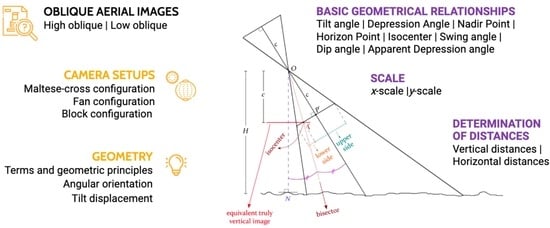
Oblique Aerial Images: Geometric Principles, Relationships and Definitions

Definition

Aerial images captured with the camera optical axis deliberately inclined with respect to the vertical are defined as oblique aerial images. Throughout the evolution of aerial photography, oblique aerial images have held a prominent place since its inception. While vertical airborne images dominated in photogrammetric applications for over a century, the advancements in photogrammetry and computer vision algorithms, coupled with the growing accessibility of oblique images in the market, have propelled the rise of oblique images in recent times. Their emergence is attributed to inherent advantages they offer over vertical images. In this entry, basic definitions, geometric principles and relationships for oblique aerial images, necessary for understanding their underlying geometry, are presented.

1. Introduction

Over the past twenty years, there has been a notable rise in the utilization of datasets featuring oblique aerial imagery. This surge can be attributed to advancements in photogrammetric and computer vision algorithms, mainly concerning image-based 3D reconstruction methods [1], the growing accessibility of these images in the market and their inherent advantages over vertical imagery. Specifically, oblique imagery offers the depiction of both vertical structures, predominantly facades, alongside horizontal elements, mimicking the human perception of scenes from a ground-level view, thus enhancing the portrayal of landscapes. Both the scientific community and multiple companies have been utilizing oblique images for diverse applications, leading to significant advancements in their automated processing [2,3]. Applications utilizing oblique aerial images include—but are not limited to—image matching [4,5,6], georeferencing [3,7,8,9], orientation and structure from motion procedures [10,11,12,13,14,15], multi-view stereo and 3D modeling pipelines [16,17,18,19,20], texture mapping [21,22,23], object detection [24,25], building identification [26,27,28], semantic segmentation of 3D city models [29] and buildings [30,31], building classification [32], extraction of post-disaster structural damages [33,34,35], historic building information modeling (HBIM) [36], reconstruction of LoD-2 building models [37], cadastral mapping [38], 3D reconstruction of canopy [39] and estimation of canopy height [40], moving car recognition [41], animal detection [42], and river surface ice quantification [43].

In this entry, basic definitions and geometric relationships for oblique aerial images, necessary for understanding their underlying geometry, are presented. The entry starts with the definition of the types of oblique aerial images and the presentation of corresponding camera setups. Subsequently, terms associated with the geometry of oblique aerial images are defined, the angular orientation in terms of azimuth, tilt and swing is presented, the displacement due to tilt is defined, and the combined effect of displacements due to relief and tilt is presented. Additionally, formulas for estimation of scales (x-scale, y-scale) in an oblique aerial image are presented, and some basic geometrical relationships among characteristic image points and angles of oblique aerial images are defined. The entry ends with the presentation of mathematical relationships that can be used for determining vertical as well as horizontal distances from a single oblique aerial image.

2. Types and Camera Setups

Aerial images taken such that the orientation of the optical axis deliberately deviates from the vertical are called oblique ones. This tilt angle is usually more than five degrees [44,45,46,47]. They are categorized as low or high oblique based on whether or not they show the apparent horizon line—the line where the earth’s surface seems to meet the sky (Section 3.1). If the apparent horizon line is visible, the image is called high oblique, else low oblique [44,45,48,49].

Besides obtaining individual oblique aerial images from either manned aerial systems or unmanned aerial vehicles (UAVs), there are multi-camera setups in the market. These systems capture either solely oblique images or a mix of oblique and vertical imagery. They employ various numbers and types of cameras, along with different acquisition setups like Maltese-cross, fan, or block configurations. A comprehensive overview of these systems and configurations can be found in [2,50,51,52,53,54]. Here, an outline of the most commonly used camera setups is given.

The most frequently employed setup is the Maltese-cross configuration (Figure 1a), typically comprising a vertical camera facing downward and four oblique ones angled towards the cardinal directions. The fan configuration (Figure 1b–d) involves aligning two or more cameras at varying angles, with their optical axes within the same vertical plane. This setup might consist of a vertical and an oblique camera or two oblique ones oriented across or along the track. Another configuration uses three cameras: one capturing vertical images while the others take oblique ones. Another way to achieve broad across-track coverage is by using a multi-lens camera with four, six, or eight lenses pointing obliquely to both sides of the flight line. Lastly, in the block configuration, typically four to six oblique cameras are arranged in a block. The overlap among these images enables their rectification and stitching to form a larger composite image.

3. Geometry of Oblique Imagery

Understanding the geometry of oblique aerial images enables accurate interpretation of visual data, aiding in the precise analysis of structures depicted in oblique imagery. Moreover, it facilitates effective surveying and mapping and helps in incorporating additional geometrical constraints in state-of-the-art workflows using oblique aerial images, like SfM and MVS. Besides, knowledge of the geometry of oblique images is a prerequisite across various disciplines besides photogrammetry, from urban planning to environmental monitoring; keeping abreast of oblique image geometry ensures compatibility with evolving technologies, such as advanced sensors and drones, optimizing data collection strategies. In this section, terms associated with oblique aerial images along with their geometric properties are defined; the angular orientation in terms of azimuth, tilt, and swing is presented; the displacement due to tilt is defined; the combined effect of relief and tilt is presented; the relationships for computing the x-scale and y-scale in an oblique aerial image are presented; and some basic geometrical relationships among characteristic points and angles in an oblique aerial image are established.

3.1. Terms and Geometric Properties

In this section, terms associated with the geometry of oblique aerial images are defined and their basic geometric properties are presented [44,45,55,56,57].

The principal plane of an oblique aerial image is the vertical plane including the camera optical axis and the vertical line from the projection center; it intersects the oblique image plane at the principal line. The latter passes through the image nadir point and the principal point. Both the principal plane and the principal line make sense only in oblique imagery. The principal line is the line of biggest inclination in an oblique aerial image. All image points that lie on lines perpendicular to the principal line correspond to the same scale, assuming horizontal ground.

The isocenter (I′) is the point where the bisector of the angle between the camera optical axis and the vertical line from the projection center intersects the oblique image plane (Figure 2 and Figure 3). It is the intersection point of the principal line and the line that results from the intersection of the oblique image plane and the plane of an assumed truly vertical image with the same projection center taken by the same camera with the same focal length (equivalent truly vertical image). The isocenter lies on the principal plane, the oblique image plane and the plane of the equivalent truly vertical image. The displacement due to tilt in an oblique image is radial with respect to the isocenter. Similarly, this term makes sense only in oblique imagery. Its main characteristic is the fact that angles measured from the isocenter of an oblique aerial image are true, i.e., they are equal to the real angles measured from the ground isocenter.

The axis of tilt—or equivalently, the isometric parallel, is the line where the oblique image plane meets the plane of an equivalent truly vertical image (Figure 3) It is perpendicular to the principal line, passing through the isocenter. The axis of tilt, like every image line perpendicular to the principal line, is a horizontal line and corresponds to zero displacement due to tilt relative to an equivalent truly vertical image. Along the axis of tilt, the image scale is constant and equals c/H (where c is the camera constant and H is the flying height), assuming horizontal ground. The axis of tilt separates the oblique image into two sides, i.e., the upper side and the lower side (Figure 2). The local scale is larger than c/H below the axis of tilt (“lower” side of image) and smaller than c/H above the axis of tilt (“upper” side of the image).

The true horizon line is the line where the horizontal plane including the perspective center meets the oblique image plane (Figure 4). It is perpendicular to the principal line and parallel to the axis of tilt. The apparent horizon line is the actual image line in which the earth’s surface appears to meet the sky. It is a real line depicted in a high oblique aerial image and appears below the fantastic true horizon line. The horizon point (K′) is the intersection of the principal line with the horizontal plane through the perspective center or, equivalently, the intersection of the principal line with the true horizon line (Figure 4).

The dip angle (δ) is the angle measured on the principal plane of an oblique aerial image between the apparent horizon line and the true horizon line. The apparent depression angle (γ) is the angle measured on the principal plane between the camera optical axis and the apparent horizon. The depression angle (θ) is the angle measured on the principal plane between the camera axis and the true horizon. Due to earth curvature and flying height, the apparent horizon appears below the true horizon; thus, the apparent depression angle incremented by the dip angle gives the depression angle (Figure 5).

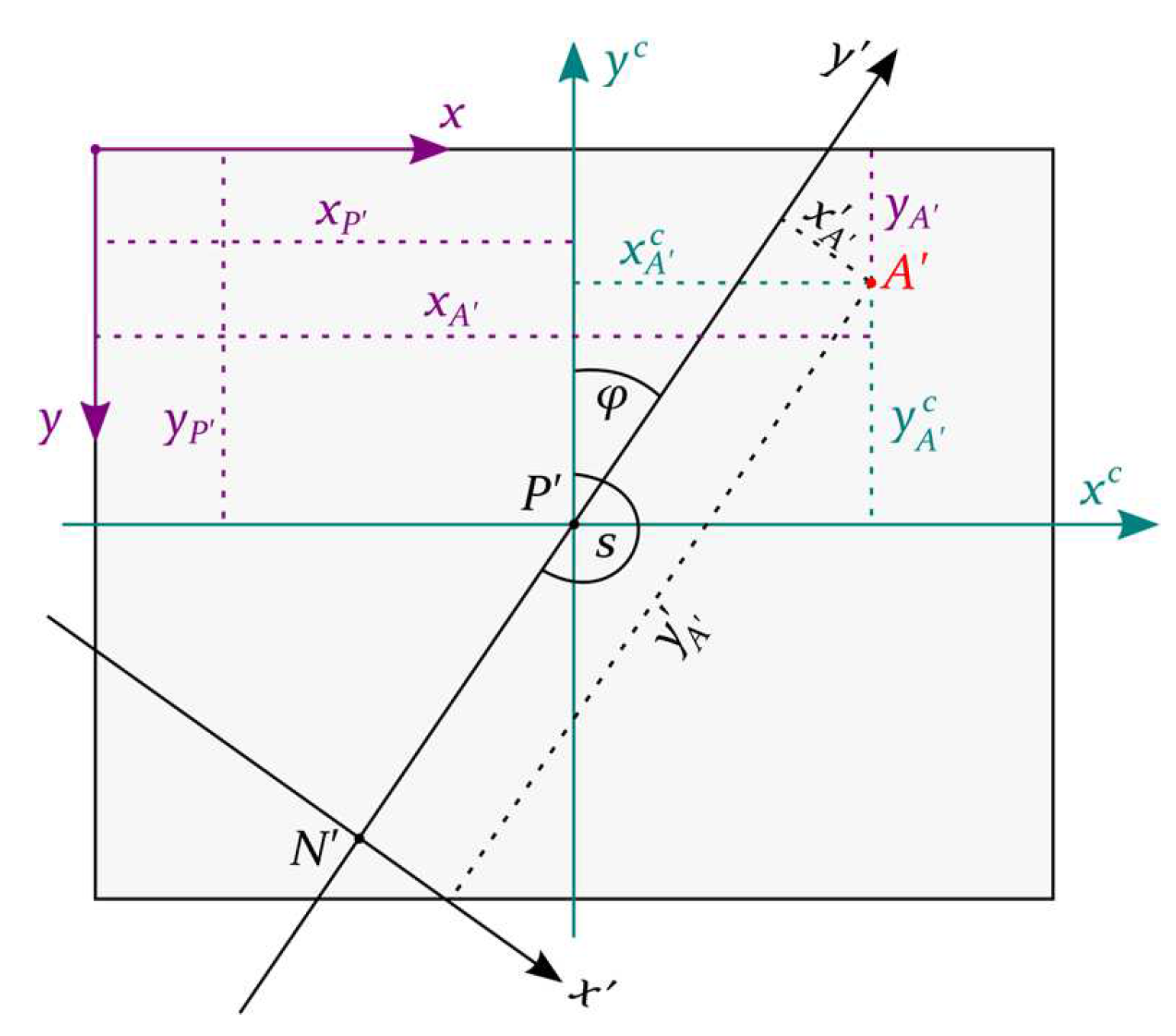
3.2. Angular Orientation in Azimuth-Tilt-Swing

The azimuth angle (a) is the clockwise horizontal angle measured about the ground nadir point from a line parallel to the ground Y-axis to the principal plane of the image. The tilt angle (t) is the angle between the vertical line from the projection center and the camera axis. The swing angle (s) is the clockwise angle measured at the oblique image plane from the positive y-axis to the principal line at the side of the image nadir point (Figure 4) [44,58]. The rotation matrix—R, expressed in angles of azimuth, tilt, and swing—is given by Equation (1) [59].

$$\mathit{R}=\left[\begin{array}{ccc}-\cos s\cdot \cos a-\sin s\cdot \cos t\cdot \sin a& \cos s\cdot \sin a-\sin s\cdot \cos t\cdot \cos a& -\sin s\cdot \sin t\\ \sin s\cdot \cos a-\cos s\cdot \cos t\cdot \sin a& -\sin s\cdot \sin a-\cos s\cdot \cos t\cdot \cos a& -\cos s\cdot \sin t\\ -\sin t\cdot \sin a& -\sin t\cdot \cos a& \cos t\end{array}\right]$$

(1)

The angles of azimuth, tilt, and swing are computed from the elements r_ij of the rotation matrix according to the set of Equation (2).

$$a={\tan }^{-1}\left(-r_{31}/-r_{32}\right); t={\cos }^{-1}\left(r_{33}\right); s={\tan }^{-1}\left(-r_{13}/-r_{23}\right)$$

(2)

3.3. Tilt Displacement

The displacement due to tilt (tilt displacement) for a point is defined as the distance from the isocenter to the image of the point in an equivalent truly vertical photograph minus the distance from the isocenter to the image of the point in the oblique photograph [49]. Image points located on the lower side of the oblique image are radially displaced away from the isocenter, thus corresponding to a larger scale than the scale that they would have in an equivalent truly vertical image. Points imaged on the upper side of the image are radially displaced towards the isocenter, thus corresponding to a smaller scale than that in an equivalent truly vertical image.

The algebraic value of the displacement due to tilt (Δr_tilt) for a point of an oblique aerial image is given by Equation (3) [49,60], where r_I is the radial distance from the isocenter to the point, c is the camera constant, t is the tilt angle, and ξ is the angle measured clockwise from the positive end of the principal line to the radial line from the isocenter to the point.

$$\Delta r_{tilt}=\frac{r_I^2\cdot {\cos }^2\xi \cdot \sin t}{c-r_I\cdot \cos \xi \cdot \sin t}$$

(3)

If the point is located on the lower side of the oblique image, its corrected radial distance from the isocenter, $r_I^c$, is computed as $r_I^c=r_I-\Delta r_{tilt}$. If the point is located on the upper side of the oblique image, its corrected radial distance from the isocenter is computed as $r_I^c=r_I+\Delta r_{tilt}$.

On the contrary, the displacement of a point due to its elevation is radial from the nadir point and always positive—that is, points elevated with respect to the datum are radially displaced outwards, away from the nadir point. The relief displacement (Δr_relief) for a point is given by Equation (4), where $r_N$ is the radial distance from the isocenter to the point, h is its elevation, and H is the flying height above the datum.

$$\Delta r_{relief}=\frac{r_N\cdot h}{H}$$

(4)

The combined effect of relief displacement and tilt displacement is illustrated in Figure 6. Each point with subscript 1 $(A_1^{\prime },B_1^{\prime },C_1^{\prime },D_1^{\prime },E_1^{\prime })$ corresponds to the position that the point would have without the effects of relief and tilt displacement (corrected position). Each point with subscript 2 $(A_2^{\prime },B_2^{\prime },C_2^{\prime },D_2^{\prime },E_2^{\prime })$ represents the position of the point after it has undergone relief displacement—that is, after it has been radially displaced outwards from the nadir point. Each point with subscript 3 $(A_3^{\prime },B_3^{\prime },C_3^{\prime },D_3^{\prime },E_3^{\prime })$ represents the position of the point after it has undergone tilt displacement (observed position of the image point). Specifically, point $A_2^{\prime }$ lies on the axis of tilt; thus, it is not displaced due to tilt, and point $A_3^{\prime }$ coincides with point $A_2^{\prime }$. Point $B_2^{\prime }$ is radially displaced away from the isocenter to be represented in position $B_3^{\prime }$, as it is located in the lower side of the image. Point $C_2^{\prime }$ is radially displaced towards the isocenter by the amount $\left(C_2^{\prime }{C}_3^{\prime }\right)$, as it lies in the upper side of the image. Points $D_2^{\prime }$ and $E_2^{\prime }$ are displaced along the principal line radially inwards and outwards with respect to the isocenter, respectively; for these points, the relief and tilt displacement are cumulative.

3.4. Scale

The scale at a point on an oblique aerial image is not the same in all directions. The scale of lines perpendicular to the principal line (x-scale) and the scale of lines parallel to the principal line (y-scale) are not the same. The scale of an oblique aerial image varies along the direction of the principal line. The scale of line segments perpendicular to the principal line is constant, whereas the scale of all the other line segments of an oblique aerial image varies. In this section, for the sake of completeness, the derivations of the well-known relationships for the computation of the scale of lines perpendicular to the principal line and infinitesimal line segments parallel to the principal line are shown. The reader may also refer to [44,61,62,63].

3.4.1. Scale of Lines Perpendicular to the Principal Line

In an oblique aerial image, the scale remains constant along each line perpendicular to the principal line. This scale along a line perpendicular to the principal line is termed as the x-scale. The x-scale increases along the principal line from the horizon point to the nadir point. Let Τ′ be the image of a world point T on the oblique photograph and let $T_1\prime$ be the projection of $T\prime$ on the principal line (Figure 7); thus, the line segment ${T\prime T}_1\prime$ is perpendicular to the principal line. The point $T_1$ is the projection of the world point T on the principal plane. Both line segments ${T\prime T}_1\prime$ and ${TT}_1$ are horizontal.

Equation (5) determines the x-scale along the line containing points Τ′ and $T_1\prime$, considering the similarity between triangles ${OT\prime T}_1\prime$ and ${OTT}_1$.

$$s_x=\frac{T\prime T_1\prime }{T{T}_1}=\frac{OT\prime }{OT}=\frac{O{T}_1\prime }{O{T}_1}$$

(5)

By trigonometric relations on the right triangles ${OP\prime T}_1\prime$ and ${O{N}_{1}T}_1$, Equations (6) and (7) are derived, where ζ is the angle formed by the camera axis and the ray to the point $T_1\prime$, and ΔH is the difference in elevation between the point T and the ground nadir point, being positive if T is above the ground nadir point N and negative if T is below the ground nadir point.

$$O{T}_1\prime =\frac{c}{\cos \zeta }$$

(6)

$$\begin{array}{c}O{T}_1=\frac{H-\Delta H}{\cos (\mathrm{t}+\zeta )}, \mathrm{if} T_1\prime \mathrm{lies} \mathrm{in} \mathrm{the} \mathrm{ray} \overrightarrow{P\prime K\prime }\\ O{T}_1=\frac{H-\Delta H}{\cos (\mathrm{t}-\zeta )}, \mathrm{if} T_1\prime \mathrm{lies} \mathrm{in} \mathrm{the} \mathrm{ray} \overrightarrow{P\prime N\prime }\end{array}$$

(7)

Using Equations (6) and (7), Equation (5) takes the following form (Equation (8)) for computation of the x-scale of a point $T\prime$ or $T_1\prime$.

$$\begin{array}{l}{s}_x=\frac{c\cos (t+\zeta )}{\left(H-\Delta H\right)\cos \zeta }, \mathrm{if} {T_1}^{\prime } \mathrm{lies} \mathrm{in} \mathrm{the} \mathrm{ray} \overrightarrow{P^{\prime }{K}^{\prime }}\\ s_x=\frac{c\cos (t-\zeta )}{\left(H-\Delta H\right)\cos \zeta }, \mathrm{if} {T_1}^{\prime } \mathrm{lies} \mathrm{in} \mathrm{the} \mathrm{ray} \overrightarrow{P^{\prime }{N}^{\prime }}\end{array}$$

(8)

Alternatively, the x-scale along a line l perpendicular to the principal line may be expressed in terms of the distance d between the true horizon line and the line l (measured parallel to the principal line); d is calculated by the set of Equation (9), which is derived considering trigonometric relations in the right triangles $O{P}^{\prime }K\prime$ and $O{P}^{\prime }{T}_1\prime$.

$$\begin{array}{l}d=K\prime P\prime -P\prime T_1\prime =c\left(\tan \theta -\tan \zeta \right), \mathrm{if} T_1\prime \mathrm{lies} \mathrm{in} \mathrm{the} \mathrm{ray} \overrightarrow{P\prime K\prime }\\ d=K\prime P\prime +P\prime T_1\prime =c\left(\tan \theta +\tan \zeta \right), \mathrm{if} T_1\prime \mathrm{lies} \mathrm{in} \mathrm{the} \mathrm{ray} \overrightarrow{P\prime N\prime }\end{array}$$

(9)

By trigonometric identity, the set of Equation (9) takes the following form (Equation (10)).

$$\begin{array}{c}\mathrm{if} T_1\prime \mathrm{lies} \mathrm{in} \mathrm{the} \mathrm{ray} \overrightarrow{P\prime K\prime }:\\ d=c\frac{\sin \left(\theta -\zeta \right)}{\cos \theta \cos \zeta }=c\frac{\sin \left(90°-t-\zeta \right)}{\cos \theta \cos \zeta }=c\frac{\sin \left(90°-\left(t+\zeta \right)\right)}{\cos \theta \cos \zeta }=c\frac{\cos \left(t+\zeta \right)}{\cos \theta \cos \zeta }\\ \mathrm{if} T_1\prime \mathrm{lies} \mathrm{in} \mathrm{the} \mathrm{ray} \overrightarrow{P\prime N\prime }:\\ d=c\frac{\sin \left(\theta +\zeta \right)}{\cos \theta \cos \zeta }=c\frac{\sin \left(90°-t+\zeta \right)}{\cos \theta \cos \zeta }=c\frac{\sin \left(90°-\left(t-\zeta \right)\right)}{\cos \theta \cos \zeta }=c\frac{\cos \left(t-\zeta \right)}{\cos \theta \cos \zeta }\end{array}$$

(10)

Substituting Equation (10) in Equation (8), the x-scale of a point or line that is perpendicular to the principal line is given by Equation (11) [44,61,62,63].

$$s_x=\frac{d\cos \theta }{H-\Delta H}$$

(11)

3.4.2. Scale of Lines Parallel to the Principal Line

The scale of a line parallel to the principal line, i.e., perpendicular to the lines of constant scale, varies along this line. The scale in a direction parallel to the principal line is called y-scale. Since the scale in the direction parallel to the principal line varies from point to point, the y-scale may be considered to be constant only for an infinitesimal distance. Let $T\prime$ and $T_2\prime$ be the images of the real world points T and $T_2$ on the oblique photograph that lie on the principal plane such that the line segment ${T\prime T}_2\prime$ lies on the principal line and the line segments ${T\prime T}_2\prime$ and ${TT}_2$ are of infinitesimal length (Figure 8). The y-scale of the infinitesimal line segment ${T\prime T}_2\prime$ is computed by Equation (12).

$$s_y=\frac{T\prime T_2\prime }{T{T}_2}$$

(12)

Equation (13) is derived by the law of sines in the triangle $T_{2}TW$ (Figure 8).

$$\frac{T{T}_2}{\sin \left(T_{2}WT\right)}=\frac{TW}{\sin \left(T{T}_{2}W\right)} \to {TT}_2=TW\frac{\sin \left(T_{2}WT\right)}{\sin \left(T{T}_{2}W\right)}$$

(13)

The line segments $OT$ and $O{T}_2$ may be considered to be parallel, as the line segment ${{\rm T}T}_2$ is infinitesimal. Thus, the angle $P{T}_{2}O$ may be considered to be equal to the angle $PTO$. Hence, the angle ${TT}_{2}W$, which is equal to the angle $P{T}_{2}O$, is computed as follows (Equation (14)).

$$\begin{array}{l}\mathrm{angle} T{T}_{2}W=\theta -\zeta , \mathrm{if} T\prime \mathrm{and} T_2\prime \mathrm{lie} \mathrm{in} \mathrm{the} \mathrm{ray} \overrightarrow{P\prime K\prime }\\ \mathrm{angle} T{T}_{2}W=\theta +\zeta , \mathrm{if} T\prime \mathrm{and} T_2\prime \mathrm{lie} \mathrm{in} \mathrm{the} \mathrm{ray} \overrightarrow{P\prime N\prime }\end{array}$$

(14)

In this way, the angle $T_{2}WT$ is computed as follows (Equation (15)).

$$\begin{array}{l}\mathrm{angle} T_{2}WT=90°+\zeta , \mathrm{if} T\prime \mathrm{and} T_2\prime \mathrm{lie} \mathrm{in} \mathrm{the} \mathrm{ray} \overrightarrow{P\prime K\prime }\\ \mathrm{angle} T_{2}WT=90°-\zeta , \mathrm{if} T\prime \mathrm{and} T_2\prime \mathrm{lie} \mathrm{in} \mathrm{the} \mathrm{ray} \overrightarrow{P\prime N\prime }\end{array}$$

(15)

Hence, Equation (13) takes the following form (Equation (16)).

$$\begin{array}{l}T{T}_2=TW\frac{\sin \left(90°+\zeta \right)}{\sin \left(\theta -\zeta \right)}, \mathrm{if} T\prime \mathrm{and} T_2\prime \mathrm{lie} \mathrm{in} \mathrm{the} \mathrm{ray} \overrightarrow{P\prime K\prime }\\ T{T}_2=TW\frac{\sin \left(90°-\zeta \right)}{\sin \left(\theta +\zeta \right)}, \mathrm{if} T\prime \mathrm{and} T_2\prime \mathrm{lie} \mathrm{in} \mathrm{the} \mathrm{ray} \overrightarrow{P\prime N\prime }\end{array}$$

(16)

Substituting the set of Equation (16) in Equation (12), Equation (17) are derived.

$$\begin{array}{l}{s}_y=\frac{T\prime T_2\prime \sin \left(\theta -\zeta \right)}{TW\sin \left(90°+\zeta \right)}, \mathrm{if} T\prime \mathrm{and} T_2\prime \mathrm{lie} \mathrm{in} \mathrm{the} \mathrm{ray} \overrightarrow{P\prime K\prime }\\ s_y=\frac{T\prime T_2\prime \sin \left(\theta +\zeta \right)}{TW\sin \left(90°-\zeta \right)}, \mathrm{if} T\prime \mathrm{and} T_2\prime \mathrm{lie} \mathrm{in} \mathrm{the} \mathrm{ray} \overrightarrow{P\prime N\prime }\end{array}$$

(17)

From the similar triangles $O{T}^{\prime }{T}_2\prime$ and $OTW$ and Equation (5), Equation (18) is derived.

$$\frac{T\prime T_2\prime }{TW}=\frac{OT\prime }{OT}=s_x$$

(18)

Substituting the set of Equation (8) in Equation (18) and substituting the result in the set of Equation (17), the set of Equation (19) is derived.

$$\begin{array}{c}\mathrm{if} T\prime \mathrm{and} T_2\prime \mathrm{lie} \mathrm{in} \mathrm{the} \mathrm{ray} \overrightarrow{P\prime K\prime }:\\ s_y=\frac{c\cos (t+\zeta )\sin \left(\theta -\zeta \right)}{\left(H-\Delta H\right)\cos \zeta \sin \left(90°+\zeta \right)}=\frac{c\sin \left(\theta -\zeta \right)\sin \left(\theta -\zeta \right)}{\left(H-\Delta H\right)\cos \zeta \cos \zeta }=\frac{c}{\left(H-\Delta H\right)}{\left(\frac{\sin \left(\theta -\zeta \right)}{\cos \zeta }\right)}^2\\ \mathrm{if} T\prime \mathrm{and} T_2\prime \mathrm{lie} \mathrm{in} \mathrm{the} \mathrm{ray} \overrightarrow{P\prime N\prime }:\\ s_y=\frac{c\cos (t-\zeta )\sin \left(\theta +\zeta \right)}{\left(H-\Delta H\right)\cos \zeta \sin \left(90°-\zeta \right)}=\frac{c\sin \left(\theta +\zeta \right)\sin \left(\theta +\zeta \right)}{\left(H-\Delta H\right)\cos \zeta \cos \zeta }=\frac{c}{\left(H-\Delta H\right)}{\left(\frac{\sin \left(\theta +\zeta \right)}{\cos \zeta }\right)}^2\end{array}$$

(19)

From Equation (10), Equation (20) are derived.

$$\begin{array}{l}\frac{\sin \left(\theta -\zeta \right)}{\cos \zeta }=\frac{d\cos \theta }{c}, \mathrm{if} T\prime \mathrm{lies} \mathrm{in} \mathrm{the} \mathrm{ray} \overrightarrow{P\prime K\prime }\\ \frac{\sin \left(\theta +\zeta \right)}{\cos \zeta }=\frac{d\cos \theta }{c}, \mathrm{if} T\prime \mathrm{lies} \mathrm{in} \mathrm{the} \mathrm{ray} \overrightarrow{P\prime N\prime }\end{array}$$

(20)

Substituting Equation (2) in Equation (19), the y-scale of the infinitesimal line segment $T^{\prime }{T}_2\prime$ (or a point $T^{\prime }$) is computed by Equation (21).

$$s_y=\frac{d^2\cdot {\cos }^2\theta }{c\left(H-\Delta H\right)}$$

(21)

Whereas the x-scale represents the scale of a point in a direction perpendicular to the principal line, the y-scale represents its scale in the direction parallel to the principal line. In the case of line segments, the x-scale represents the scale of a line segment that is perpendicular to the principal line, whereas the y-scale represents the scale of a line segment that is parallel to the principal line, provided that the latter is of infinitesimal length, as the y-scale can be considered constant only for an infinitesimal distance. These scales can be used in order to compute ground distances. The x-scale and the y-scale differ by the factor dcosθ/c (i.e., s_y/s_x = dcosθ/c), and the angle θ is positive and smaller than 90°, s_y < s_x if d < c, whereas s_y > s_x if d > c. Thus, for a specific image, the smaller the distance d between a point and the true horizon line is, the smaller the y-scale is compared to the x-scale, assuming that d < c. In the case that d > c for a specific image, the bigger d is, the bigger the y-scale is compared to the x-scale. The length of a line segment that is neither perpendicular nor parallel to the principal line can be roughly computed by obtaining the lengths of its components, perpendicular and parallel to the principal line, using the x-scale and the y-scale, respectively. However, it should be noted that since the scale is constant only along lines perpendicular to the principal line and the y-scale assumes an infinitesimal distance, ground distances of line segments that are not perpendicular to the principal line may be only approximately computed using the scales given by Equations (11) and (21).

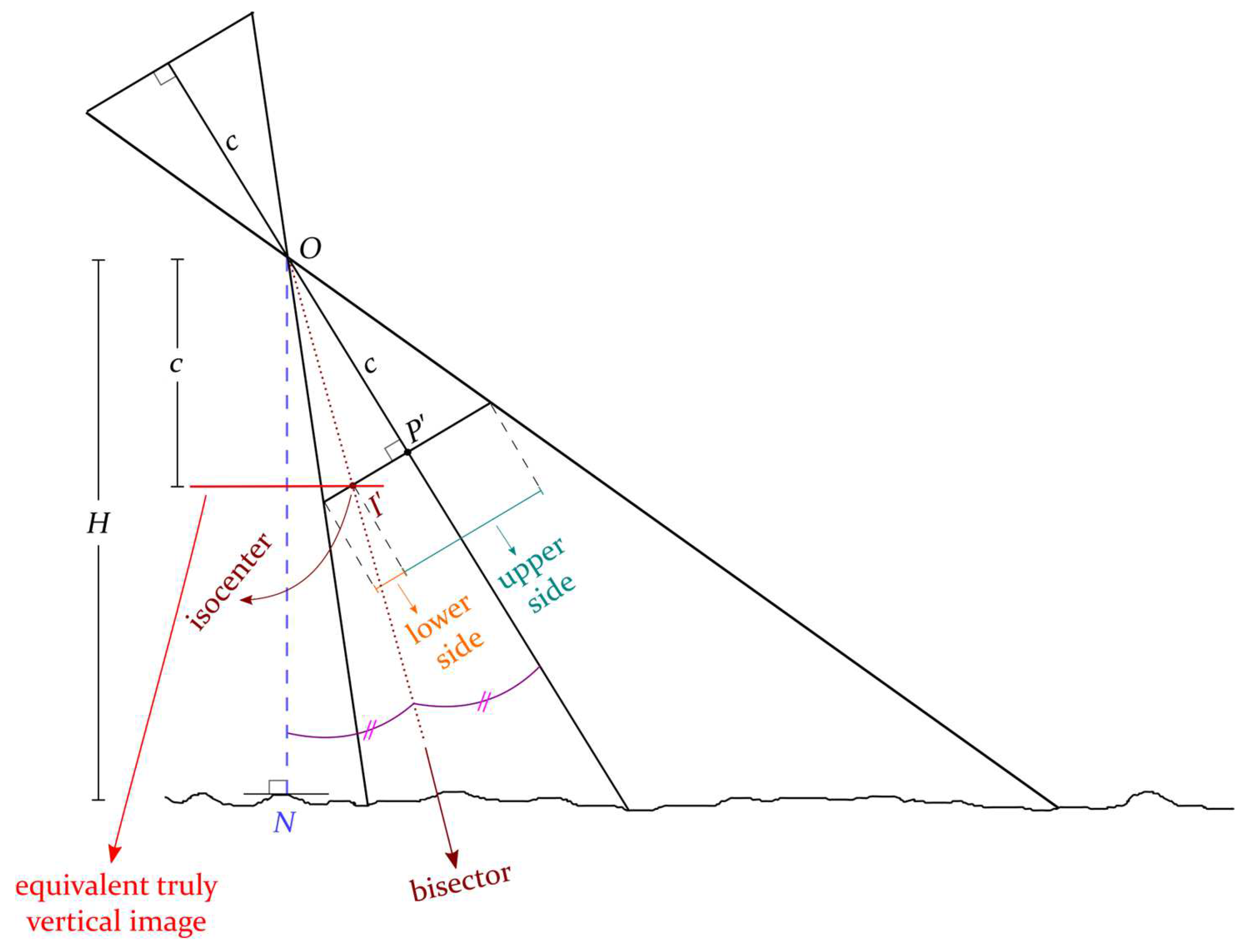
3.5. Basic Geometrical Relationships

In this section, basic mathematical relationships among the principal point, the horizon point, the nadir point, the isocenter, the tilt angle, the depression angle, the apparent depression angle and the swing angle as well as between the flying height and the dip angle are presented, and their derivations are shown in this section for the sake of completeness. These mathematical relationships are particularly useful for determining the geometry of a single oblique aerial image. For instance, if the nadir point is automatically estimated from an oblique aerial image of known interior orientation (e.g., via the method presented in [3,64]), the tilt angle, the depression angle, the swing angle, the horizon point, and the isocenter may also be calculated using the relationships presented in this section.

3.5.1. Tilt and Depression Angles, Nadir Point, and Horizon Point

The depression angle is the complement of the tilt angle (Figure 8); thus, it is calculated by Equation (22).

$$\theta =90°-t$$

(22)

The depression angle may be calculated as a function of the distance between the principal point and the horizon point (Figure 8) according to Equation (23).

$$K\prime P\prime =c\tan \theta \to \theta =\arctan \left(\frac{K\prime P\prime }{c}\right)$$

(23)

The tilt angle may be calculated using the distance between the principal point and the image of the nadir point (Figure 8) using Equation (24).

$$P\prime N\prime =c\tan t \to t=\arctan \left(\frac{P\prime N\prime }{c}\right)$$

(24)

Taking into account the fact that the tilt angle is the complement of the depression angle, the distance between the principal point and the image of the nadir point may, alternatively, be expressed as a function of the depression angle, according to Equation (25).

$$P\prime N\prime =c\tan \left(90°-\theta \right) \to P\prime N\prime =c\cot \theta$$

(25)

The distance between the horizon point and the nadir point is calculated by Equation (26) as a function of the depression angle or by Equation (27) as a function of the tilt angle (Figure 8).

$$K\prime N\prime =K\prime P\prime +P\prime N\prime \to K\prime N\prime =c\tan \theta +c\cot \theta \to K\prime N\prime =c\left(\tan \theta +\cot \theta \right)$$

(26)

$$K\prime N\prime =c\left(\cot t+\tan t\right)$$

(27)

3.5.2. Isocenter

The distance between the isocenter and the principal point is calculated using Equation (28) as a function of the tilt angle (Figure 5) or by Equation (29) as a function of the depression angle.

$$P\prime I\prime =c\tan \left(\frac{t}{2}\right)$$

(28)

$$P\prime I\prime =c\tan \left(\frac{90°-\theta }{2}\right) \to P\prime I\prime =c\tan \left(45°-\frac{\theta }{2}\right)$$

(29)

The distance between the horizon point and the isocenter is computed by Equation (30), as a function of the depression angle (Figure 5), using Equations (23) and (29).

$$K\prime {\rm I}\prime =K\prime P\prime +P\prime I\prime \to K\prime {\rm I}\prime =c\left(\tan \theta +\tan \left(45°-\frac{\theta }{2}\right)\right)$$

(30)

Equation (31) is derived by mathematical operations and trigonometric identities.

$$\tan \left(45°-\frac{\theta }{2}\right)=\frac{1-\sin \theta }{\cos \theta }$$

(31)

By substituting Equation (31) in Equation (30), Equation (32) is finally derived for the calculation of the distance between the horizon point and the isocenter as a function of the depression angle.

$$K\prime {\rm I}\prime =c\left(\frac{\sin \theta }{\cos \theta }+\frac{1-\sin \theta }{\cos \theta }\right) \to K\prime {\rm I}\prime =\frac{c}{\cos \theta }$$

(32)

The distance between the horizon point and the isocenter may also be calculated by Equation (33) as a function of the tilt angle using Equation (32) and taking into account the fact that the tilt angle is the complement of the depression angle.

$$K\prime {\rm I}\prime =\frac{c}{\sin t}$$

(33)

3.5.3. Swing Angle

The swing angle may be calculated according to the set of Equation (34) using the coordinates of the nadir point in the image coordinate system centered at the principal point (x^c, y^c) (Figure 9).

$$s=\left\{\begin{array}{l}90°+\arctan \left|\frac{x_{N\prime }^c}{y_{N\prime }^c}\right| \mathrm{if} x_{N\prime }^c\le 0\\ 90°-\arctan \left|\frac{x_{N\prime }^c}{y_{N\prime }^c}\right| \mathrm{if} x_{N\prime }^c>0\end{array}\right\}$$

(34)

The coordinates of the nadir point in the image coordinate system centered at the principal point (x^c, y^c) are computed bases on its pixel coordinates and those of the principal point. Assuming that the image coordinate system in pixels (x, y) has its origin at the top-left pixel, the swing angle is computed by the set of Equation (35) as a function of the pixel coordinates of the principal point and the nadir point (Figure 9).

$$s=\left\{\begin{array}{l}90°+\arctan \left|\frac{x_{N\prime }-x_{P\prime }}{y_{P\prime }-y_{N\prime }}\right| \mathrm{if} x_{N\prime }\le x_{P\prime }\\ 90°-\arctan \left|\frac{x_{N\prime }-x_{P\prime }}{y_{P\prime }-y_{N\prime }}\right| \mathrm{if} x_{N\prime }>x_{P\prime }\end{array}\right\}$$

(35)

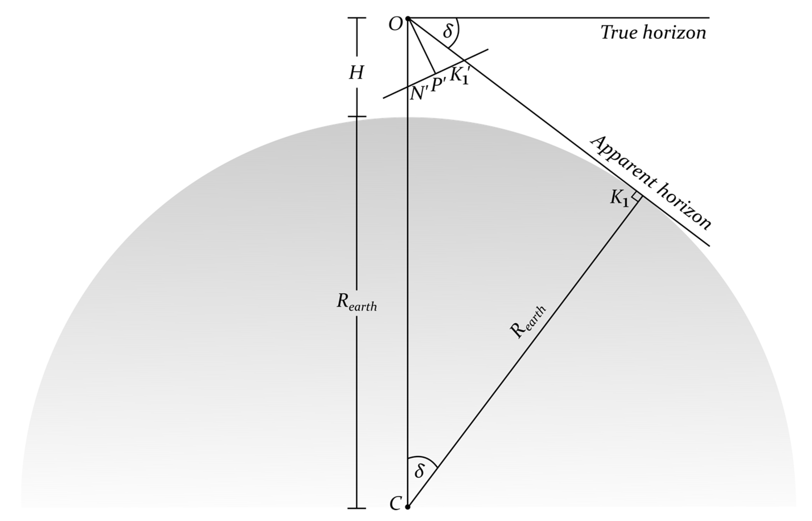
3.5.4. Dip Angle

The dip angle is geometrically calculated using the right triangle OCK₁ (Figure 10), according to Equation (36), where OK₁ is the trace of the apparent horizon in the principal plane and R_earth is the radius of the earth, assuming that the earth is approximated by a sphere.

$$\tan \delta =\frac{O{K}_1}{R_{earth}} \to \delta =\arctan \left(\frac{O{K}_1}{R_{earth}}\right)$$

(36)

In the right triangle OCK₁, Equation (37) is derived.

$$O{K}_1=\sqrt{{\left(R_{earth}+H\right)}^2-{R_{earth}}^2} \to O{K}_1=\sqrt{2R_{earth}H+H^2}$$

(37)

Substituting Equation (37) in Equation (36), Equation (38) is derived for the calculation of the dip angle.

$$\delta =\arctan \left(\frac{\sqrt{2R_{earth}H+H^2}}{R_{earth}}\right)$$

(38)

Considering that the radius of earth is constant, the dip angle is a function of the flying height and increases with it. By ignoring the term H² of Equation (38), as it is very small compared to the quantity 2R_earthH, and substituting the average value of the radius of the earth, the dip angle is approximated by Equation (39) [44].

$$\delta =106.5\sqrt{H},\delta \mathrm{in} \mathrm{seconds}, H \mathrm{in} \mathrm{meters}$$

(39)

3.5.5. Apparent Depression Angle

The apparent depression angle is calculated by Equation (40), where K₁′ is the point of intersection of the apparent horizon line and the principal line (Figure 5).

$$\tan \gamma =\frac{P\prime K_1\prime }{c} \to \gamma =\arctan \left(\frac{P\prime K_1\prime }{c}\right)$$

(40)

Equation (41) expresses the relationship between the apparent depression angle, the depression angle, and the dip angle (Figure 5).

$$\theta =\gamma +\delta$$

(41)

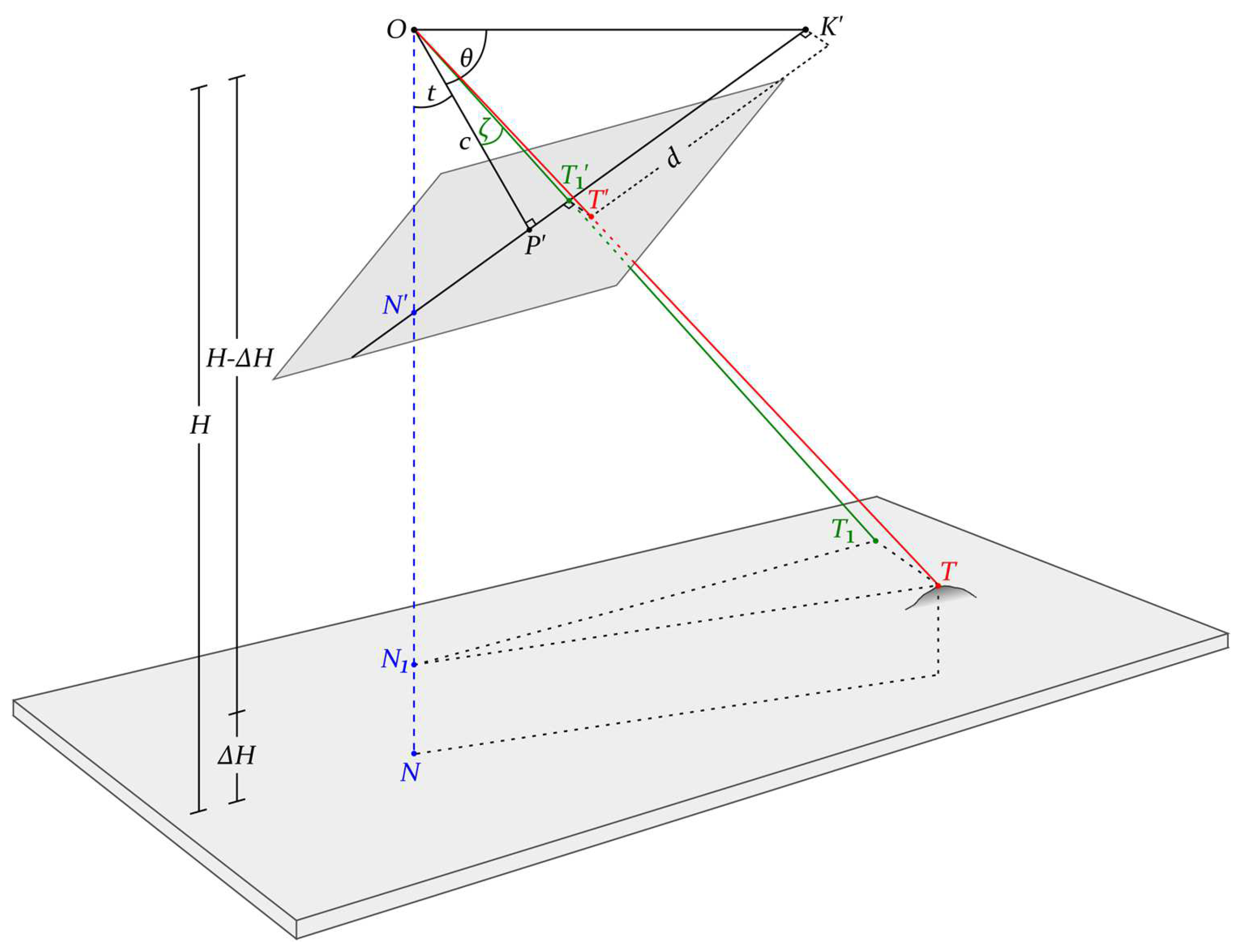
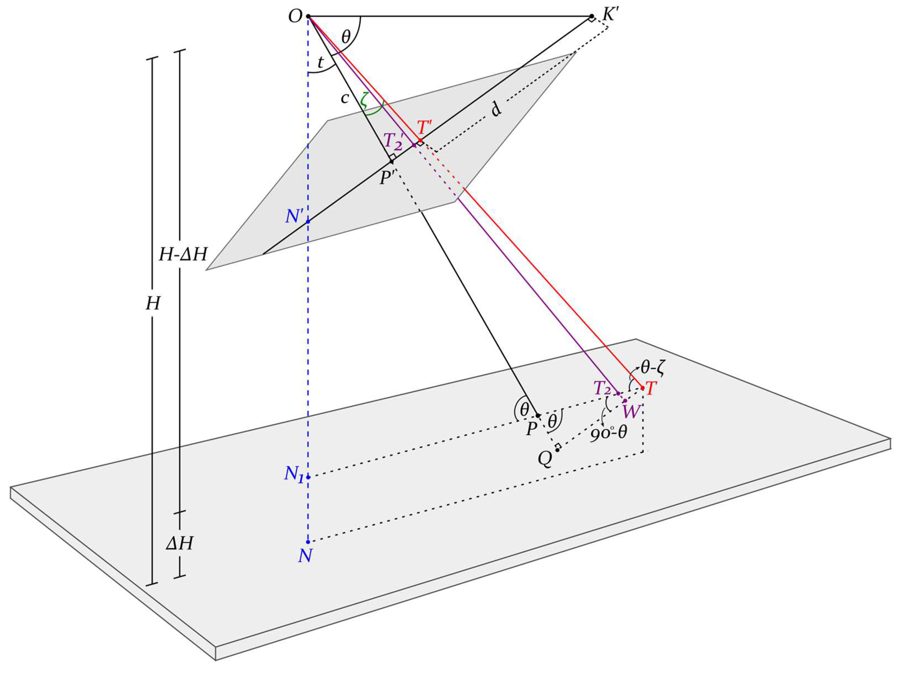
4. Determination of Distances

In this section, the mathematical relationships for estimating vertical and horizontal distances from a single oblique aerial image are outlined. The prerequisite for the monocular derivation of such metric information from an oblique image is the knowledge of the following: (i) the nadir point of the image; (ii) the camera interior orientation; and (iii) the flying height measured from the bottom point of the vertical object in the case of measuring a vertical distance or the flying height measured from the two points of same elevation in the case of measuring a horizontal distance. The nadir point can be automatically determined via the method presented in [3,64].

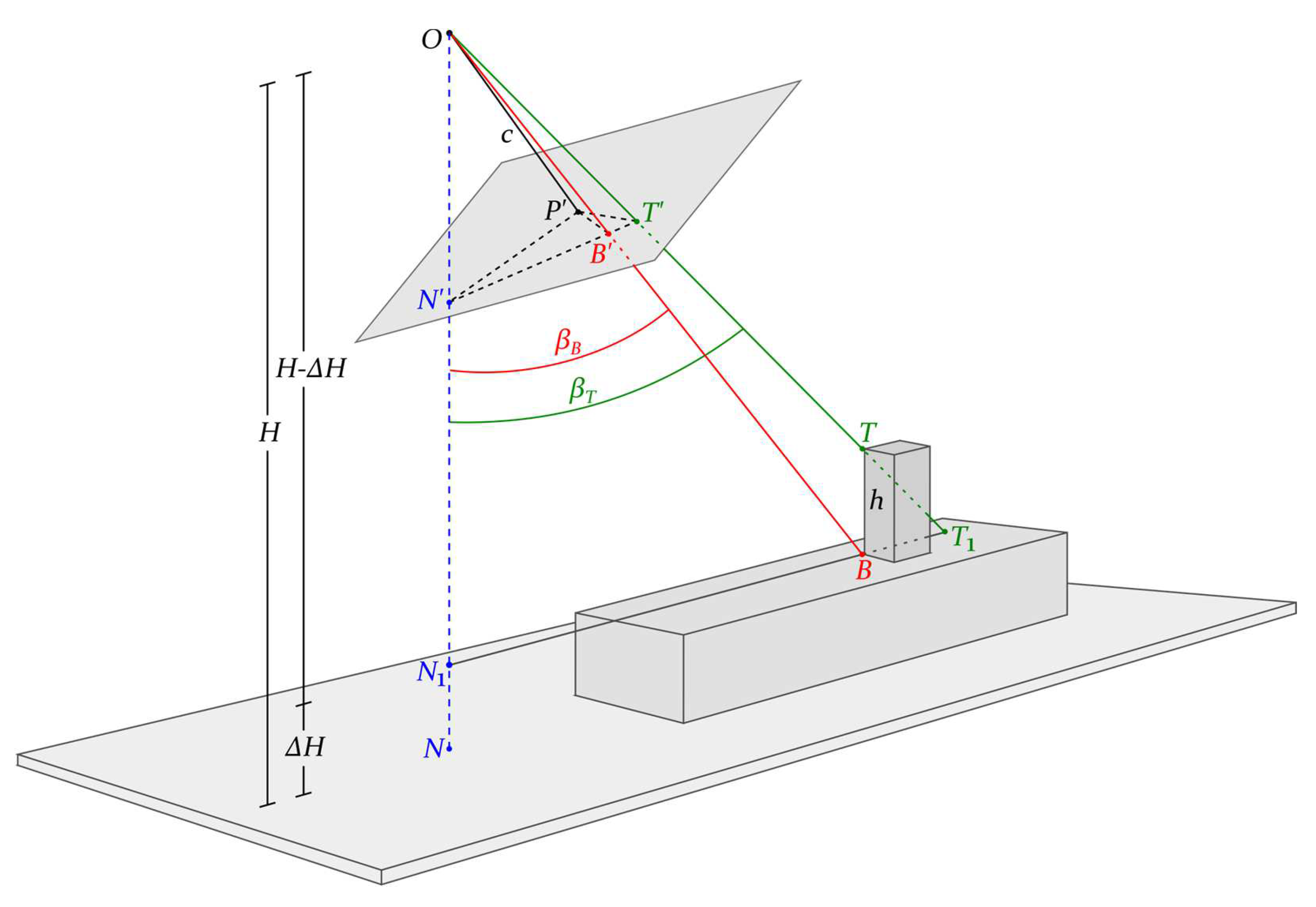
4.1. Vertical Distances

In [65], the height of a vertical object is computed from a single undistorted image using knowledge of the vanishing line of the horizontal direction, as well as the nadir point and image measurements of the top and bottom point of the vertical object, along with one object of known height for which the top and base are imaged. This is a well-established relationship that is mainly adopted for the case of terrestrial images, for which knowledge of the height of a reference small object depicted in such images is generally available. In [66], measurements of vertical distances from a single oblique image are made using knowledge of all camera settings, flight parameters as well as detailed digital terrain models (DTMs) and digital surface models (DSMs). In this section, a mathematical model for measuring vertical distances from a single oblique image is proved anew. The main motivation for proving anew such a relationship is the computation of the height of objects from a single oblique aerial image for which neither the exterior orientation parameters are available nor for which the height of a reference object is known. The external reference information required by the relationship presented in this section is the flying height measured from the bottom point of the vertical object, which, in the case of an oblique aerial image, is generally more easily available than the height of a reference object depicted in the image.

Specifically, the relationship presented in this section differs from the one proved in [66] on the grounds that it does not require knowledge of the camera exterior orientation parameters and availability of detailed DTMs/DSMs. Hence, it may also be applied in cases in which such data are not available. Similarly to the relationship presented in this section, the one derived in [65] does not require any camera exterior orientation information. The relationship presented in this section differs from the one derived in [65] in the initial data. The relationship used in [65] assumes knowledge of the height of a vertical object for which the top and base are imaged, whereas the relationship derived in this section assumes knowledge of the flying height measured from the bottom point of the vertical object. In addition to the image nadir point (which is also a prerequisite of the relationship presented in this section), the relationship presented in [65] assumes knowledge of the vanishing line of the horizontal direction. However, this is not a major difference, as knowledge of the image nadir point permits the determination of the true horizon line assuming known camera interior orientation parameters. This is achieved through estimation of the tilt angle, computation of the distance between the horizon point and the nadir point, computation of the coordinates of the horizon point, and estimation of the equation of the horizon line.

The mathematical model that can be used for computing the height of a vertical object from a single oblique aerial image is presented in the following, based on detailed proof in the doctoral dissertation of [3]. In Figure 11, Β′ and Τ′ are the projections of the bottom point B and the top point T, respectively, of an edge of a vertical object in an oblique aerial image taken at a flying height H above a specific datum. ΔH is the elevation difference between the datum plane and the bottom point of the vertical object (point B), being positive if B is above the datum plane and negative if B is below the datum plane. In Figure 11, it is assumed that the flying height is measured from the surface directly below the aerial platform, i.e., the datum plane is the horizontal plane that contains the ground nadir point N. H − ΔH is the flying height measured from the bottom point of the vertical object, i.e., the vertical distance between the camera projection center and the horizontal plane containing the bottom point of the vertical object to be measured. This is the quantity that is required by the formula which calculates the height of a vertical object. In the case that H is the flying height above a typical datum and practically refers to the Z coordinate of the camera projection center (e.g., orthometric height in the World Geodetic System 1984—WGS 84 datum), ΔH refers to the Z coordinate of the bottom point of the vertical object to be measured, which may be obtained by an online earth observation application, like Google Earth, and then H − ΔH may be calculated. In the case that H has been measured from the surface directly below the aerial platform and, as a result, ΔH refers to the elevation difference between the ground nadir point and the bottom point of the vertical object that is being measured, the difference H − ΔH may also be obtained by an online application like Google Earth, provided that the region vertically under the aerial platform can be located in the map.

The height (h) of the vertical object of interest is calculated according to Equation (42), using the similar triangles ON₁T₁ and TBT₁ (Figure 11), where N₁ is the intersection of the horizontal plane containing the bottom point B with the vertical line from the perspective center and T₁ is the intersection of the horizontal plane containing the bottom point B with the optical ray to the top point T.

$$h=\left(H-\Delta H\right)\frac{B{T}_1}{N_1{T}_1}$$

(42)

The distance BT₁ is calculated by Equation (43), where β_Β is the angle between the optical ray to the bottom point B of the vertical object and the vertical line from the projection center and β_Τ is the angle between the optical ray to the top point T of the vertical object and the vertical line from the projection center.

$$B{T}_1=N_1{T}_1-N_{1}B \to B{T}_1=\left(H-\Delta H\right)\left(\tan {\beta }_T-\tan {\beta }_B\right)$$

(43)

By substituting Equation (43) into Equation (42), Equation (44) is derived, and it computes the height of the vertical object.

$$h=\left(H-\Delta H\right)\left(1-\frac{\tan {\beta }_B}{\tan {\beta }_T}\right)$$

(44)

The cosine of the angle β_Β is computed via Equation (45) using the law of cosines in the triangle OΒ′Ν′.

$$\cos {\beta }_B=\frac{{\left(OB\prime \right)}^2+{\left(ON\prime \right)}^2-{\left(B\prime N\prime \right)}^2}{2\left(OB\prime \right)\left(ON\prime \right)}$$

(45)

The tangent of the aforementioned angle is estimated using Equation (46).

$$\tan {\beta }_B=\frac{\sqrt{1-{\cos }^2{\beta }_B}}{\cos {\beta }_B} \to \tan {\beta }_B=\frac{\sqrt{4{\left(OB\prime \right)}^2{\left(ON\prime \right)}^2-{\left[{\left(OB\prime \right)}^2+{\left(ON\prime \right)}^2-{\left(B\prime N\prime \right)}^2\right]}^2}}{{\left(OB\prime \right)}^2+{\left(ON\prime \right)}^2-{\left(B\prime N\prime \right)}^2}$$

(46)

The tangent of the angle β_Τ is calculated in a similar way according to Equation (47).

$$\tan {\beta }_T=\frac{\sqrt{4{\left(OT\prime \right)}^2{\left(ON\prime \right)}^2-{\left[{\left(OT\prime \right)}^2+{\left(ON\prime \right)}^2-{\left(T\prime N\prime \right)}^2\right]}^2}}{{\left(OT\prime \right)}^2+{\left(ON\prime \right)}^2-{\left(T\prime N\prime \right)}^2}$$

(47)

Equations (48)–(50) are derived using the right triangles OP′B′, OP′T′, and OP′N.

$$ON\prime =\sqrt{c^2+{\left(P\prime N\prime \right)}^2}$$

(48)

$$OB\prime =\sqrt{c^2+{\left(P\prime B\prime \right)}^2}$$

(49)

$$OT\prime =\sqrt{c^2+{\left(P\prime T\prime \right)}^2}$$

(50)

By substituting Equations (46)–(50) in Equation (44), the height of a vertical object is estimated using Equation (51). The image coordinates used in Equation (51) are those corrected from systematic errors (e.g., radial and tangential distortion).

$$\begin{array}{c}h=\left(H-\Delta H\right)\left(1-\frac{\frac{\sqrt{4\left(c^2+{\left(P\prime B\prime \right)}^2\right)\left(c^2+{\left(P\prime N\prime \right)}^2\right)-{\left[2c^2+{\left(P\prime B\prime \right)}^2+{\left(P\prime N\prime \right)}^2-{\left(B\prime N\prime \right)}^2\right]}^2}}{2c^2+{\left(P\prime B\prime \right)}^2+{\left(P\prime N\prime \right)}^2-{\left(B\prime N\prime \right)}^2}}{\frac{\sqrt{4\left(c^2+{\left(P\prime T\prime \right)}^2\right)\left(c^2+{\left(P\prime N\prime \right)}^2\right)-{\left[2c^2+{\left(P\prime T\prime \right)}^2+{\left(P\prime N\prime \right)}^2-{\left(T\prime N\prime \right)}^2\right]}^2}}{2c^2+{\left(P\prime T\prime \right)}^2+{\left(P\prime N\prime \right)}^2-{\left(T\prime N\prime \right)}^2}}\right)\\ \begin{array}{c}\\ \begin{array}{c}\begin{array}{l}{\left(P\prime B\prime \right)}^2={(x_{B\prime }-x_{P\prime })}^2+{(y_{B\prime }-y_{P\prime })}^2\\ {\left(P\prime N\prime \right)}^2={(x_{N\prime }-x_{P\prime })}^2+{(y_{N\prime }-y_{P\prime })}^2\\ {\left(B\prime N\prime \right)}^2={(x_{N\prime }-x_{B\prime })}^2+{(y_{N\prime }-y_{B\prime })}^2\\ {\left(P\prime T\prime \right)}^2={(x_{T\prime }-x_{P\prime })}^2+{(y_{T\prime }-y_{P\prime })}^2\\ {\left(T\prime N\prime \right)}^2={(x_{N\prime }-x_{T\prime })}^2+{(x_{N\prime }-y_{T\prime })}^2\end{array}\end{array} \mathrm{where}\\ \end{array}\left\{\begin{array}{l}{x}_{B\prime },y_{B\prime },x_{T\prime },y_{T\prime }:\\ \mathrm{the} \mathrm{image} \mathrm{coordinates} \mathrm{of} \mathrm{the} \mathrm{bottom}\\ \mathrm{and} \mathrm{the} \mathrm{top} \mathrm{point} \mathrm{of} \mathrm{the} \mathrm{vertical} \mathrm{object}\\ x_{N\prime },y_{N\prime }:\\ \mathrm{the} \mathrm{image} \mathrm{coordinates} \mathrm{of} \mathrm{the} \\ \mathrm{nadir} \mathrm{point}\\ x_{P\prime },y_{P\prime }:\\ \mathrm{the} \mathrm{image} \mathrm{coordinates} \mathrm{of} \mathrm{the} \\ \mathrm{principal} \mathrm{point} \end{array}\right\}\\ \begin{array}{l}\Delta H>0 \mathrm{if} \mathrm{the} \mathrm{datum} \mathrm{plane} \mathrm{is} \mathrm{lower} \mathrm{in} \mathrm{elevation} \mathrm{than} \mathrm{the} \mathrm{bottom} \mathrm{of} \mathrm{the} \mathrm{vertical} \mathrm{object}\\ \Delta H<0 \mathrm{if} \mathrm{the} \mathrm{datum} \mathrm{plane} \mathrm{is} \mathrm{higher} \mathrm{in} \mathrm{elevation} \mathrm{than} \mathrm{the} \mathrm{bottom} \mathrm{of} \mathrm{the} \mathrm{vertical} \mathrm{object}\end{array}\end{array}$$

(51)

4.2. Horizontal Distances

The estimation of horizontal distances from a single oblique aerial image is based on the computation of ground coordinates in a local coordinate system. The computation of ground coordinates in such a local ground coordinate system (hereinafter referred to as auxiliary ground coordinate system) has been presented and proved by the photogrammetric community [44,49]. In this section, for the scope of completeness, the derivation of the formulas that compute horizontal coordinates in the local auxiliary ground coordinates system is also presented.

The calculation of horizontal coordinates in the auxiliary ground coordinate system requires the use of an auxiliary image coordinate system. For defining the latter, it is assumed that the image has been corrected from systematic errors (e.g., lens distortion) or that systematic errors are insignificant and can be ignored. The auxiliary image coordinate system has its origin at the nadir point. The y axis coincides with the principal line, while the x-axis is perpendicular to the principal line, hence forming a horizontal line (Figure 12). It has been proven that the coordinates of an image point A′ in the aforementioned auxiliary image coordinate system are computed using Equation (52) [49], where the angle φ is a function of the swing angle s: φ = s − 180° and assuming that the origin of the image coordinate system in pixels (x, y) is located at the top left pixel.

$$\begin{array}{c}x{\prime }_{A\prime }=\left(x_{A\prime }-x_{P\prime }\right)\cos \phi -\left(y_{P\prime }-y_{A\prime }\right)\sin \phi \\ y{\prime }_{A\prime }=\left(x_{A\prime }-x_{P\prime }\right)\sin \phi +\left(y_{P\prime }-y_{A\prime }\right)\cos \phi +c\tan t\end{array}$$

(52)

The origin of the auxiliary ground coordinate system is located at the ground nadir point, while the X′ and Y′ axes are on the same vertical planes with those of the auxiliary image coordinate system, maintaining the same positive directions as them [3,44,49]. The X′ and Y′ coordinates of Point A in this system are calculated through the set of Equation (53) and have the same signs as its auxiliary image coordinates x′ and y′, respectively.

$$X{\prime }_A=\left\{\begin{array}{l}\left|\frac{\left(H-\Delta H\right)x{\prime }_{A\prime }\cos t}{c-y{\prime }_{A\prime }\sin t\cos t}\right| \mathrm{if} x{\prime }_{A\prime }\ge 0\\ -\left|\frac{\left(H-\Delta H\right)x{\prime }_{A\prime }\cos t}{c-y{\prime }_{A\prime }\sin t\cos t}\right| \mathrm{if} x{\prime }_{A\prime }<0\end{array}\right\} Y{\prime }_A=\left\{\begin{array}{l}\left|\frac{\left(H-\Delta H\right)y{\prime }_{A\prime }{\cos }^{2}t}{c-y{\prime }_{A\prime }\sin t\cos t}\right| \mathrm{if} y{\prime }_{A\prime }\ge 0\\ -\left|\frac{\left(H-\Delta H\right)y{\prime }_{A\prime }{\cos }^{2}t}{c-y{\prime }_{A\prime }\sin t\cos t}\right| \mathrm{if} y{\prime }_{A\prime }<0\end{array}\right\}$$

(53)

If the camera tilt angle t, used in the set of Equation (53) is not known a priori, it may be calculated through Equation (24), provided that the principal point and camera constant are known and the image nadir point has been determined (e.g., through the method presented in [3,64]).

The distance between two points A and C is calculated by Equation (54) after the determination of the coordinates of A and C in the auxiliary ground coordinate system, i.e., (X′_A, Y′_A) and (X′_C, Y′_C), respectively.

$$d=\sqrt{{\left(X{\prime }_C-X{\prime }_A\right)}^2+{\left(Y{\prime }_C-Y{\prime }_A\right)}^2}$$

(54)

5. Conclusions

In this entry, basic definitions and geometric relationships for oblique aerial images have been presented. Specifically, the well-established classification of oblique aerial images into low and high oblique ones has been presented, the camera configurations for capturing datasets containing oblique aerial images have been summarized, and basic terms associated with oblique aerial images along with their geometric properties and relationships have been outlined. Furthermore, mathematical relationships for computing vertical and horizontal distances from a single oblique aerial image have been established. While the measurement of horizontal distances by a method similar to the one presented in this entry has already been outlined by the photogrammetric community since the 20th century, the mathematical model presented in this entry for the determination of vertical distances has been proven anew and may be used instead of other well-established relationships for measuring the height of a vertical object. The mathematical models for determining vertical and horizontal distances may be used in combination with a nadir point detection technique, for the establishment of an automated framework for measuring vertical and horizontal distances from a single oblique image with unknown exterior orientation parameters and unavailable GCP measurements.

References

- Verykokou, S.; Ioannidis, C. An Overview on Image-Based and Scanner-Based 3D Modeling Technologies. Sensors 2023, 23, 596. [Google Scholar] [CrossRef]
- Verykokou, S.; Ioannidis, C. Oblique Aerial Images: A Review Focusing on Georeferencing Procedures. Int. J. Remote Sens. 2018, 39, 3452–3496. [Google Scholar] [CrossRef]
- Verykokou, S.A. Georeferencing Procedures for Oblique Aerial Images. Ph.D. Thesis, National Technical University of Athens, Athens, Greece, 2020. [Google Scholar] [CrossRef]
- Hu, H.; Ding, Y.; Zhu, Q.; Wu, B.; Xie, L.; Chen, M. Stable Least-Squares Matching for Oblique Images Using Bound Constrained Optimization and a Robust Loss Function. J. Photogramm. Remote Sens. 2016, 118, 53–67. [Google Scholar] [CrossRef]
- Wang, C.; Chen, J.; Chen, J.; Yue, A.; He, D.; Huang, Q.; Zhang, Y. Unmanned Aerial Vehicle Oblique Image Registration Using an ASIFT-Based Matching Method. J. Appl. Remote Sens. 2018, 12, 025002. [Google Scholar] [CrossRef]
- Zhang, Q.; Zheng, S.; Zhang, C.; Wang, X.; Li, R. Efficient Large-Scale Oblique Image Matching Based on Cascade Hashing and Match Data Scheduling. Pattern Recognit. 2023, 138, 109442. [Google Scholar] [CrossRef]
- Zhao, H.; Zhang, B.; Wu, C.; Zuo, Z.; Chen, Z.; Bi, J. Direct Georeferencing of Oblique and Vertical Imagery in Different Coordinate Systems. J. Photogramm. Remote Sens. 2014, 95, 122–133. [Google Scholar] [CrossRef]
- Geniviva, A.; Faulring, J.; Salvaggio, C. Automatic Georeferencing of Imagery from High-Resolution, Low-Altitude, Low-Cost Aerial Platforms. In Proceedings of the Geospatial InfoFusion and Video Analytics IV; and Motion Imagery for ISR and Situational Awareness II, Baltimore, MD, USA, 19 June 2014; Volume 9089, pp. 101–109. [Google Scholar]
- Verykokou, S.; Ioannidis, C. Automatic Rough Georeferencing of Multiview Oblique and Vertical Aerial Image Datasets of Urban Scenes. Photogramm. Rec. 2016, 31, 281–303. [Google Scholar] [CrossRef]
- Xie, L.; Hu, H.; Wang, J.; Zhu, Q.; Chen, M. An Asymmetric Re-Weighting Method for the Precision Combined Bundle Adjustment of Aerial Oblique Images. J. Photogramm. Remote Sens. 2016, 117, 92–107. [Google Scholar] [CrossRef]
- Verykokou, S.; Ioannidis, C. A Photogrammetry-Based Structure from Motion Algorithm Using Robust Iterative Bundle Adjustment Techniques. Ann. Photogramm. Remote Sens. Spat. Inf. Sci. 2018, 4, 73–80. [Google Scholar] [CrossRef]
- Verykokou, S.; Ioannidis, C. A Global Photogrammetry-Based Structure from Motion Framework: Application in Oblique Aerial Images. In Proceedings of the FIG Working Week 2019, Hanoi, Vietnam, 22–26 April 2019; FIG: Hanoi, Vietnam, 2019. [Google Scholar]
- Verykokou, S.; Ioannidis, C. Exterior Orientation Estimation of Oblique Aerial Images Using SfM-Based Robust Bundle Adjustment. Int. J. Remote Sens. 2020, 41, 7233–7270. [Google Scholar] [CrossRef]
- Jiang, S.; Jiang, C.; Jiang, W. Efficient Structure from Motion for Large-Scale UAV Images: A Review and a Comparison of SfM Tools. J. Photogramm. Remote Sens. 2020, 167, 230–251. [Google Scholar] [CrossRef]
- Liang, Y.; Yang, Y.; Fan, X.; Cui, T. Efficient and Accurate Hierarchical SfM Based on Adaptive Track Selection for Large-Scale Oblique Images. Remote Sens. 2023, 15, 1374. [Google Scholar] [CrossRef]
- Wu, B.; Xie, L.; Hu, H.; Zhu, Q.; Yau, E. Integration of Aerial Oblique Imagery and Terrestrial Imagery for Optimized 3D Modeling in Urban Areas. J. Photogramm. Remote Sens. 2018, 139, 119–132. [Google Scholar] [CrossRef]
- Nesbit, P.R.; Hugenholtz, C.H. Enhancing UAV–SfM 3D Model Accuracy in High-Relief Landscapes by Incorporating Oblique Images. Remote Sens. 2019, 11, 239. [Google Scholar] [CrossRef]
- Liu, J.; Zhang, L.; Wang, Z.; Wang, R. Dense Stereo Matching Strategy for Oblique Images That Considers the Plane Directions in Urban Areas. IEEE Trans. Geosci. Remote Sens. 2020, 58, 5109–5116. [Google Scholar] [CrossRef]
- Pepe, M.; Fregonese, L.; Crocetto, N. Use of SfM-MVS Approach to Nadir and Oblique Images Generated Throught Aerial Cameras to Build 2.5D Map and 3D Models in Urban Areas. Geocarto Int. 2022, 37, 120–141. [Google Scholar] [CrossRef]
- Oniga, V.-E.; Breaban, A.-I.; Pfeifer, N.; Diac, M. 3D Modeling of Urban Area Based on Oblique UAS Images—An End-to-End Pipeline. Remote Sens. 2022, 14, 422. [Google Scholar] [CrossRef]
- Frommholz, D.; Linkiewicz, M.; Meissner, H.; Dahlke, D.; Poznanska, A. Extracting Semantically Annotated 3DBuilding Models with Textures from Oblique Aerial Imagery. Int. Arch. Photogramm. Remote Sens. Spat. Inf. Sci. 2015, 40, 53–58. [Google Scholar] [CrossRef]
- Kang, J.; Deng, F.; Li, X.; Wan, F. Automatic Texture Reconstruction of 3D City Model from Oblique Images. Int. Arch. Photogramm. Remote Sens. Spat. Inf. Sci. 2016, 41, 341–347. [Google Scholar] [CrossRef]
- Zhou, G.; Bao, X.; Ye, S.; Wang, H.; Yan, H. Selection of Optimal Building Facade Texture Images From UAV-Based Multiple Oblique Image Flows. IEEE Trans. Geosci. Remote Sens. 2021, 59, 1534–1552. [Google Scholar] [CrossRef]
- Shen, H.; Lin, D.; Song, T. Object Detection Deployed on UAVs for Oblique Images by Fusing IMU Information. IEEE Geosci. Remote Sens. Lett. 2022, 19, 6505305. [Google Scholar] [CrossRef]
- Zachar, P.; Kurczyński, Z.; Ostrowski, W. Application of Machine Learning for Object Detection in Oblique Aerial Images. Int. Arch. Photogramm. Remote Sens. Spat. Inf. Sci. 2022, 43, 657–663. [Google Scholar] [CrossRef]
- Cai, Y.; Ding, Y.; Zhang, H.; Xiu, J.; Liu, Z. Geo-Location Algorithm for Building Targets in Oblique Remote Sensing Images Based on Deep Learning and Height Estimation. Remote Sens. 2020, 12, 2427. [Google Scholar] [CrossRef]
- Zhang, L.; Wang, G.; Sun, W. Automatic Identification of Building Structure Types Using Unmanned Aerial Vehicle Oblique Images and Deep Learning Considering Facade Prior Knowledge. Int. J. Digit. Earth 2023, 16, 3348–3367. [Google Scholar] [CrossRef]
- Liang, Y.; Fan, X.; Yang, Y.; Li, D.; Cui, T. Oblique View Selection for Efficient and Accurate Building Reconstruction in Rural Areas Using Large-Scale UAV Images. Drones 2022, 6, 175. [Google Scholar] [CrossRef]
- Wilk, Ł.; Mielczarek, D.; Ostrowski, W.; Dominik, W.; Krawczyk, J. Semantic Urban Mesh Segmentation Based on Aerial Oblique Images and Point Clouds Using Deep Learning. Int. Arch. Photogramm. Remote Sens. Spat. Inf. Sci. 2022, 43, 485–491. [Google Scholar] [CrossRef]
- Khoshboresh-Masouleh, M.; Alidoost, F.; Arefi, H. Multiscale Building Segmentation Based on Deep Learning for Remote Sensing RGB Images from Different Sensors. J. Appl. Remote Sens. 2020, 14, 034503. [Google Scholar] [CrossRef]
- Mao, Z.; Huang, X.; Gong, Y.; Xiang, H.; Zhang, F. A Dataset and Ensemble Model for Glass Façade Segmentation in Oblique Aerial Images. IEEE Geosci. Remote Sens. Lett. 2022, 19, 6513305. [Google Scholar] [CrossRef]
- Meng, C.; Song, Y.; Ji, J.; Jia, Z.; Zhou, Z.; Gao, P.; Liu, S. Automatic Classification of Rural Building Characteristics Using Deep Learning Methods on Oblique Photography. Build. Simul. 2022, 15, 1161–1174. [Google Scholar] [CrossRef]
- Vetrivel, A.; Gerke, M.; Kerle, N.; Vosselman, G. Identification of Structurally Damaged Areas in Airborne Oblique Images Using a Visual-Bag-of-Words Approach. Remote Sens. 2016, 8, 231. [Google Scholar] [CrossRef]
- Kakooei, M.; Baleghi, Y. A Two-Level Fusion for Building Irregularity Detection in Post-Disaster VHR Oblique Images. Earth Sci. Inf. 2020, 13, 459–477. [Google Scholar] [CrossRef]
- Zhang, R.; Li, H.; Duan, K.; You, S.; Liu, K.; Wang, F.; Hu, Y. Automatic Detection of Earthquake-Damaged Buildings by Integrating UAV Oblique Photography and Infrared Thermal Imaging. Remote Sens. 2020, 12, 2621. [Google Scholar] [CrossRef]
- Martínez-Carricondo, P.; Carvajal-Ramírez, F.; Yero-Paneque, L.; Agüera-Vega, F. Combination of Nadiral and Oblique UAV Photogrammetry and HBIM for the Virtual Reconstruction of Cultural Heritage. Case Study of Cortijo Del Fraile in Níjar, Almería (Spain). Build. Res. Inf. 2020, 48, 140–159. [Google Scholar] [CrossRef]
- Wang, F.; Zhou, G.; Hu, H.; Wang, Y.; Fu, B.; Li, S.; Xie, J. Reconstruction of LoD-2 Building Models Guided by Façade Structures from Oblique Photogrammetric Point Cloud. Remote Sens. 2023, 15, 400. [Google Scholar] [CrossRef]
- Šafář, V.; Potůčková, M.; Karas, J.; Tlustý, J.; Štefanová, E.; Jančovič, M.; Cígler Žofková, D. The Use of UAV in Cadastral Mapping of the Czech Republic. ISPRS Int. J. Geo-Inf. 2021, 10, 380. [Google Scholar] [CrossRef]
- Díaz, G.M.; Mohr-Bell, D.; Garrett, M.; Muñoz, L.; Lencinas, J.D. Customizing Unmanned Aircraft Systems to Reduce Forest Inventory Costs: Can Oblique Images Substantially Improve the 3D Reconstruction of the Canopy? Int. J. Remote Sens. 2020, 41, 3480–3510. [Google Scholar] [CrossRef]
- Li, M.; Shamshiri, R.R.; Schirrmann, M.; Weltzien, C.; Shafian, S.; Laursen, M.S. UAV Oblique Imagery with an Adaptive Micro-Terrain Model for Estimation of Leaf Area Index and Height of Maize Canopy from 3D Point Clouds. Remote Sens. 2022, 14, 585. [Google Scholar] [CrossRef]
- Yang, C.; Zhang, F.; Gao, Y.; Mao, Z.; Li, L.; Huang, X. Moving Car Recognition and Removal for 3D Urban Modelling Using Oblique Images. Remote Sens. 2021, 13, 3458. [Google Scholar] [CrossRef]
- Lamprey, R.; Pope, F.; Ngene, S.; Norton-Griffiths, M.; Frederick, H.; Okita-Ouma, B.; Douglas-Hamilton, I. Comparing an Automated High-Definition Oblique Camera System to Rear-Seat-Observers in a Wildlife Survey in Tsavo, Kenya: Taking Multi-Species Aerial Counts to the next Level. Biol. Conserv. 2020, 241, 108243. [Google Scholar] [CrossRef]
- Pei, C.; She, Y.; Loewen, M. Deep Learning Based River Surface Ice Quantification Using a Distant and Oblique-Viewed Public Camera. Cold Reg. Sci. Technol. 2023, 206, 103736. [Google Scholar] [CrossRef]
- Moffitt, F.H.; Mikhail, E.M. Photogrammetry; Harper & Row Inc.: New York, NY, USA, 1980. [Google Scholar]
- Trorey, L.G. Handbook of Aerial Mapping and Photogrammetry; Cambridge University Press: Cambridge, UK, 1952. [Google Scholar]
- Höhle, J. Photogrammetric Measurements in Oblique Aerial Images. Photogramm. Fernerkund. Geoinf. 2008, 1, 7–14. [Google Scholar]
- Shufelt, J.A. Performance Evaluation and Analysis of Monocular Building Extraction from Aerial Imagery. IEEE Trans. Pattern Anal. Mach. Intell. 1999, 21, 311–326. [Google Scholar] [CrossRef]
- Moffitt, F.H. Elements of Photogrammetry; International Textbook Company: Scranton, PA, USA, 1962. [Google Scholar]
- Wolf, P.R. Elements of Photogrammetry: With Air Photo Interpretation and Remote Sensing, 2nd ed.; McGraw-Hill: New York, NY, USA, 1983; ISBN 9780070713451. [Google Scholar]
- Petrie, G. Systematic Oblique Aerial Photography Using Multiple Digital Frame Cameras. Photogramm. Eng. Remote Sens. 2009, 75, 102–107. [Google Scholar]
- Lemmens, M. Digital Oblique Aerial Cameras (1): A Survey of Features and Systems. GIM Int. 2014. Available online: https://repository.tudelft.nl/islandora/object/uuid:a2548e3d-2408-4eba-8e67-69c504d5cfec?collection=research (accessed on 13 December 2023).
- Lemmens, M. Digital Oblique Aerial Cameras (2): A Survey of Features and Systems. GIM Int. 2014. Available online: http://www.gdmc.nl/publications/2014/Digital_Oblique_Aerial_Cameras_2.pdf (accessed on 13 December 2023).
- Rupnik, E.; Nex, F.; Remondino, F. Oblique multi-camera systems—Orientation and dense matching issues. Int. Arch. Photogramm. Remote Sens. Spat. Inf. Sci. 2014, 40, 107114. [Google Scholar] [CrossRef]
- Remondino, F.; Gerke, M. Oblique Aerial Imagery—A Review. In Proceedings of the Photogrammetric Week’15, Stuttgart, Germany, 7–11 September 2015; Wichmann/VDE Verlag: Belin, Germany, 2015. [Google Scholar]
- Introduction to Oblique Photogrammetry; Hydrographic Office Navy Department & Photographic Intelligence Center—Division of Naval Intelligence—Navy Department: Arlington, VA, USA, 1945.
- Manual of Photogrammetry, 2nd ed.; American Society of Photogrammetry: Washington, DC, USA, 1952.
- Paine, D.P.; Kiser, J.D. Aerial Photography and Image Interpretation, 3rd ed.; Wiley: Hoboken, NJ, USA, 2012; ISBN 9780470879382. [Google Scholar]
- Punmia, B.C.; Jain, A.K.; Jain, A.K. Higher Surveying, Surveying-III; Laxmi Publications Pvt. Ltd.: New Delhi, India, 2005; ISBN 9788170088257. [Google Scholar]
- Dewitt, B.A. Initial Approximations for the Three-Dimensional Conformal Coordinate Transformation. Photogramm. Eng. Remote Sens. 1996, 62, 79–83. [Google Scholar]
- Misulia, M.G. A Derivation for the Image Displacement Due to Tilt. Photogramm. Eng. 1946, pp. 461–463. Available online: https://www.asprs.org/wp-content/uploads/pers/1946journal/dec/1946_dec_461-463.pdf (accessed on 13 December 2023).
- Lane, B.B. Scales of Oblique Photographs. Photogramm. Eng. 1950, pp. 409–414. Available online: https://www.asprs.org/wp-content/uploads/pers/1950journal/jun/1950_jun_409-414.pdf (accessed on 13 December 2023).
- Moffitt, F.H. Photogrammetry; International Textbook Company: Scranton, PA, USA, 1967. [Google Scholar]
- Wolf, P.R. Elements of Photogrammetry; McGraw-Hill Inc.: New York, NY, USA, 1984. [Google Scholar]
- Verykokou, S.; Ioannidis, C. Exterior orientation estimation of oblique aerial imagery using vanishing points. Int. Arch. Photogramm. Remote Sens. Spat. Inf. Sci. 2016, 41, 123–130. [Google Scholar] [CrossRef]
- Hartley, R.; Zisserman, A. Multiple View Geometry in Computer Vision; Cambridge University Press: Cambridge, UK, 2003; ISBN 9780521540513. [Google Scholar]
- Molinari, M.; Medda, S.; Villani, S. Vertical Measurements in Oblique Aerial Imagery. IJGI ISPRS Int. J. Geo-Inf. 2014, 3, 914–928. [Google Scholar] [CrossRef]
Disclaimer/Publisher’s Note: The statements, opinions and data contained in all publications are solely those of the individual author(s) and contributor(s) and not of MDPI and/or the editor(s). MDPI and/or the editor(s) disclaim responsibility for any injury to people or property resulting from any ideas, methods, instructions or products referred to in the content. |
© 2024 by the authors. Licensee MDPI, Basel, Switzerland. This article is an open access article distributed under the terms and conditions of the Creative Commons Attribution (CC BY) license (https://creativecommons.org/licenses/by/4.0/).
Share and Cite
Verykokou, S.; Ioannidis, C. Oblique Aerial Images: Geometric Principles, Relationships and Definitions. Encyclopedia 2024, 4, 234-255. https://doi.org/10.3390/encyclopedia4010019
Verykokou S, Ioannidis C. Oblique Aerial Images: Geometric Principles, Relationships and Definitions. Encyclopedia. 2024; 4(1):234-255. https://doi.org/10.3390/encyclopedia4010019
Chicago/Turabian StyleVerykokou, Styliani, and Charalabos Ioannidis. 2024. "Oblique Aerial Images: Geometric Principles, Relationships and Definitions" Encyclopedia 4, no. 1: 234-255. https://doi.org/10.3390/encyclopedia4010019
APA StyleVerykokou, S., & Ioannidis, C. (2024). Oblique Aerial Images: Geometric Principles, Relationships and Definitions. Encyclopedia, 4(1), 234-255. https://doi.org/10.3390/encyclopedia4010019