
Techniques for Theoretical Prediction of Immunogenic Peptides


Department of Biological Sciences, University of South Carolina, Columbia, SC 29208, USA
†
Retired.
Encyclopedia 2024, 4(1), 600-621; https://doi.org/10.3390/encyclopedia4010038
Submission received: 4 February 2024
/
Revised: 10 March 2024
/
Accepted: 15 March 2024
/
Published: 19 March 2024
(This article belongs to the Section Biology & Life Sciences)
Definition
:Small peptides are an important component of the vertebrate immune system. They are important molecules for distinguishing proteins that originate in the host from proteins derived from a pathogenic organism, such as a virus or bacterium. Consequently, these peptides are central for the vertebrate host response to intracellular and extracellular pathogens. Computational models for prediction of these peptides have been based on a narrow sample of data with an emphasis on the position and chemical properties of the amino acids. In past literature, this approach has resulted in higher predictability than models that rely on the geometrical arrangement of atoms. However, protein structure data from experiment and theory are a source for building models at scale, and, therefore, knowledge on the role of small peptides and their immunogenicity in the vertebrate immune system. The following sections introduce procedures that contribute to theoretical prediction of peptides and their role in immunogenicity. Lastly, deep learning is discussed as it applies to immunogenetics and the acceleration of knowledge by a capability for modeling the complexity of natural phenomena.
1. Background on Immunological Peptides
The adaptive immune system of vertebrates is a system that includes cells and molecules whose role is to distinguish self from the outside world (non-self). Therefore, a vertebrate host has the potential for detecting and clearing pathogenic organisms from its organ systems. A major component of adaptive immunity involves a linear chain of amino acids: the small peptides [1]. The small peptide is of interest since the host immune system relies on it as a marker for a determination on whether a protein originates from itself or instead of a foreign source, such as a virus or bacterium [2]. This system can also identify its own cells as foreign if they are genetically altered by a process that causes production of unfamiliar molecules [3,4].
These peptides of interest are formed by cleavage of proteins in cells of the host, and they form the basis for the cellular processes of immune surveillance, and identification of pathogens and cells that operate outside their normal genetic programming [3,5,6,7]. When adaptive immunity falsely identifies a peptide derived from a protein that is essential to the individual as not originating from that individual, a phenomenon referred to as autoimmunity occurs [8,9,10,11]. A generalized example of autoimmunity is where a subset of T cells [12,13], a name that references their development in the thymus [14,15], falsely detects small peptides as presented on the surface of cells as originating from non-self and subsequently signals the immune system to eliminate these cells in the host [16,17,18].
The mechanism for peptide detection is reliant on molecular binding between the peptide and a major histocompatibility complex (MHC) receptor that is expressed in the majority of cells of a vertebrate [19,20,21]. Nearly all cells of the canonical vertebrate express MHC Class 1 cell surface receptors that are capable of presenting peptides of an intracellular origin, while a subset of cell types of the immune system express MHC Class 2 cell surface receptors for presentation of peptides of an intercellular origin.
Furthermore, the mechanism described above is refined by training the T cells to perform as specialists so that they disfavor any attack on normal cells, while favoring the proliferation of the T cells that have developed to attack non-self [14,21]. This is not a deterministic process, however. The dictates of probability are present in biological systems, including: (1) the generation of genetic diversity across the various MHC receptor types, (2) the cleavage process for generation of small peptides from a protein, (3) the timeliness of the immune response to molecular evidence of a pathogen, (4) the binding strength of peptides to an MHC receptor, and (5) the requisite sample of peptides for detection of a pathogen. This system is in contrast to a human designed system (engineered) in which the structure and function originate from an artificial design and a low tolerance for the prior mentioned variability.
The aggregate of past collections of immunological peptide data is not representative of the total space of these peptides [3,21]. For example, only a small proportion of MHC molecules have been studied for their association with small peptides. This sampling problem is related to the allelic distribution of the MHC molecules. While there are about a dozen genetic loci in clusters that code for a MHC protein receptor, the number of alleles among these loci is very high as compared to the other genetic loci in the typical vertebrate genome. In the human population, the expected number of alleles for the MHC loci is estimated in the thousands [3,22]. Correspondingly, these loci are active genetic sites of evolutionary change and generation of diversity, and—unlike the other regions of the genome—this genetic diversity has been undiminished at the genetic level by the putative bottleneck that reduced our effective population size to mere thousands of individuals [23]. Likewise, the study of immunological peptides has generally been restricted to that of the human population and animal models that serve as a proxy in the study of biomedicine and livestock [21].
Moreover, there is a preference for MHC class type as a result of model feasibility. The MHC Class 1 receptor is generally favored over that of Class 2 in modeling the MHC-peptide association, partly because in MHC Class 1, some of the amino acids of the peptide are confined in pockets of the MHC receptor [1,3,24,25]. This has led to predictive models of MHC-peptide (pMHC) binding that parameterize the position and chemical type of the amino acids of these peptides [21,26]. These models have exceeded the predictiveness as compared to models based solely on geometrical data of the atomic arrangements [3]. However, the geometrical features are expected to contribute to insight on pMHC binding and models for predicting an adaptive immune response.
Recently, artificial neural networks and related machine language approaches have led to advances in knowledge of protein structure and the potential for modeling the association between proteins and other molecules [21,26,27,28,29]. These methods are capable of highly predictive models that incorporate disparate kinds of data, such as in the use of both geometrical and chemical features in estimating the binding affinity for an MHC receptor with a peptide [21]. Moreover, they are highly efficient in the case where modeling is dependent on a very large number of parameters, as commonly observed in the interactions of biological molecules. Consequently, the deep learning approaches have shown success in the prediction of protein structure across a broad sampling of the clades of living organisms [30]. These approaches are complemented through the analysis of metrics, preferably with a level of interpretability, that are capable of estimating the geometrical similarity among proteins [31,32,33].
As a whole, the study of immunogenetics relies on collecting data and building models as expected in the pursuit of knowledge [21,34]. Deep learning is applicable to these goals, for which the data collection is extensive and there is a theoretical basis for the system of interest. Ideally, this kind of scientific practice is expected to lead to a meaningful synthesis that is unmired by a collector’s fondness for naming schemes and ungrounded collations of terms and studies [35]. The latter perspective resembles the practice of creating images of science, akin to an art form, that sometimes occur in the disciplines of natural science while not achieving the aim of extending knowledge through the purposeful modeling of natural phenomena [36].
2. Metrics of Peptide Structure Similarity
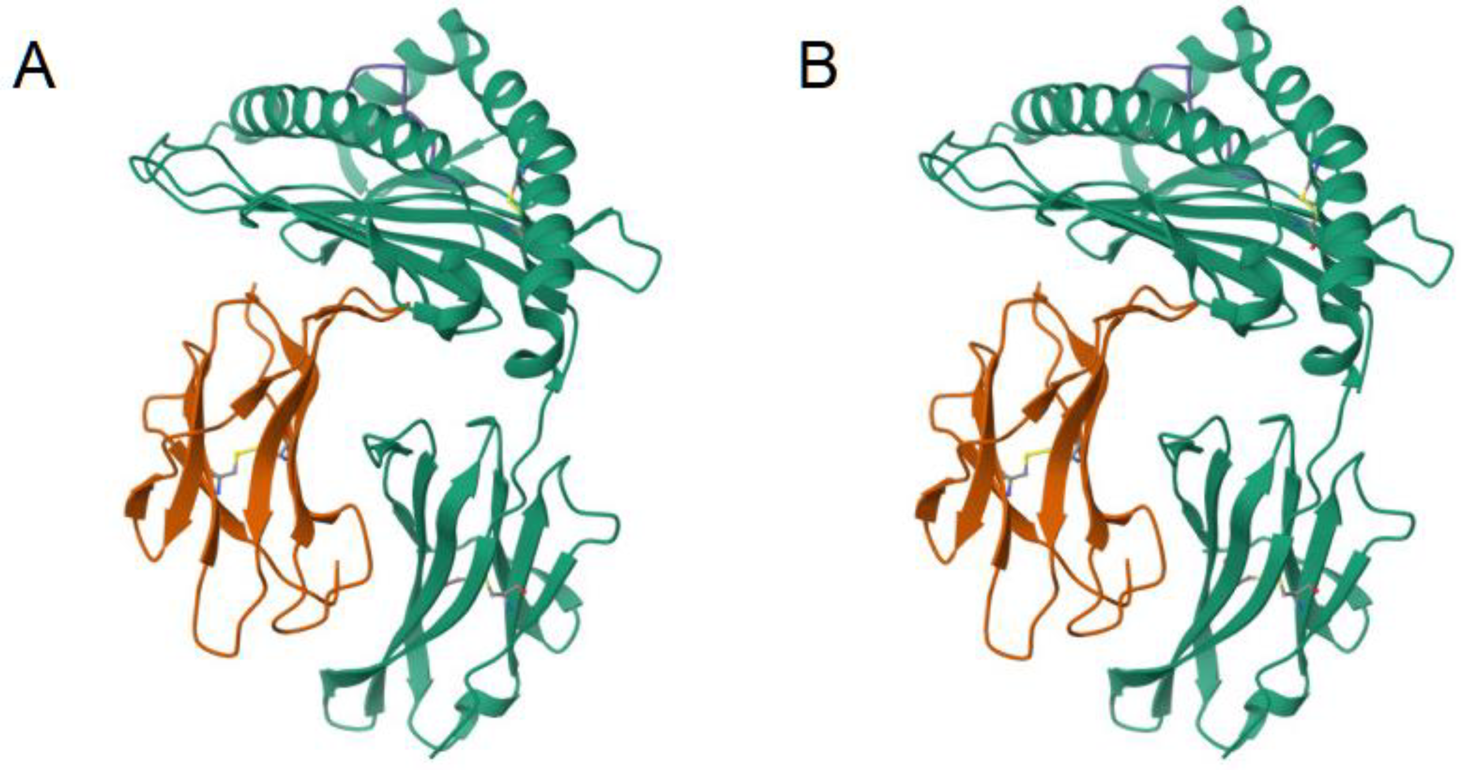
There are a large number of methods for quantifying the geometrical similarity among proteins [37]. In particular, one method is by the template modeling score (TM score), which is based on an algorithm, and a performant implementation in computer code, for measuring the similarity between any two protein molecules (Figure 1) [31]. Furthermore, the compiled program from this open source code computes a root mean-square deviation (RMSD) metric, a similar measure to the TM score, but, where the latter method is less sensitive to the non-local interactions in a molecular topology, along with the advantage of model invariance to the size of the protein. However, the RMSD metric is also an interpretable metric.
Given any cellular protein, there is empirical support for a range of TM scores that are meaningful as a description of protein structure similarity, and, likewise, for dissimilarity. A value above 0.5 is regarded as a significant result of similarity, while a value less than 0.17 represents a comparison that is essentially indistinguishable from a randomly selected comparison [38]. The values of this metric are further bounded by 0 and 1.
Figure 1.
Ribbon diagrams of the 3D atomic structure of an MHC Class 1 receptor as bound to a peptide [39]. These protein structures appear mostly identical, so a score based on their 3D similarity is expected be high in value [31]. (A) This panel shows the bound peptide AH1 (6L9M). Adapted from [40]. (B) In this case, the bound peptide is A5 (6L9N). Adapted from [41].

Furthermore, the TM score is applicable to the analysis of small peptides. For instance, it is possible to sample protein structure data [30], select all unordered pairs of proteins for comparison, and then find an empirical distribution of values for this metric. This procedure may be used to establish values of significance for this metric. Appendix A describes a procedure for obtaining and verifying data for biological proteins [42], including any subsequent prediction of their three-dimensional structure.
3. Peptide Structure Analysis in Immunogenetics
3.1. Significance Levels for TM Score
The TM score metric is a powerful tool for measuring structural similarities among proteins [31]. This metric can be applied to the study of small peptides. However, in the case of small peptides, the significance levels are not yet established for the TM score metric. However, these levels can be empirically estimated through computational analysis of randomly selected pairs of small peptides, such as in a sliding window analysis based on the residues in protein structure data, or, alternatively, by generation of sequence data via simulation. These findings would establish a baseline for the analysis of small peptides as derived from clinical and other data—such as from an emergent pathogen—leading to an expectation of the numbers and types of amino acid changes that lead to adaptation for evasion of host immunity. Note that these procedures are based on the sampling of linear peptides by a host immune system, as in its detection by a type of T cell, but the role of the B cell in immunity is a separate problem wherein the effective sampling of polypeptides by the immune system is often dependent on geometric proximity of amino acid residues and is therefore, not reliant on a linear arrangement of amino acids for the detection of non-self molecules.
3.2. Local versus Global Factors of Protein Structure
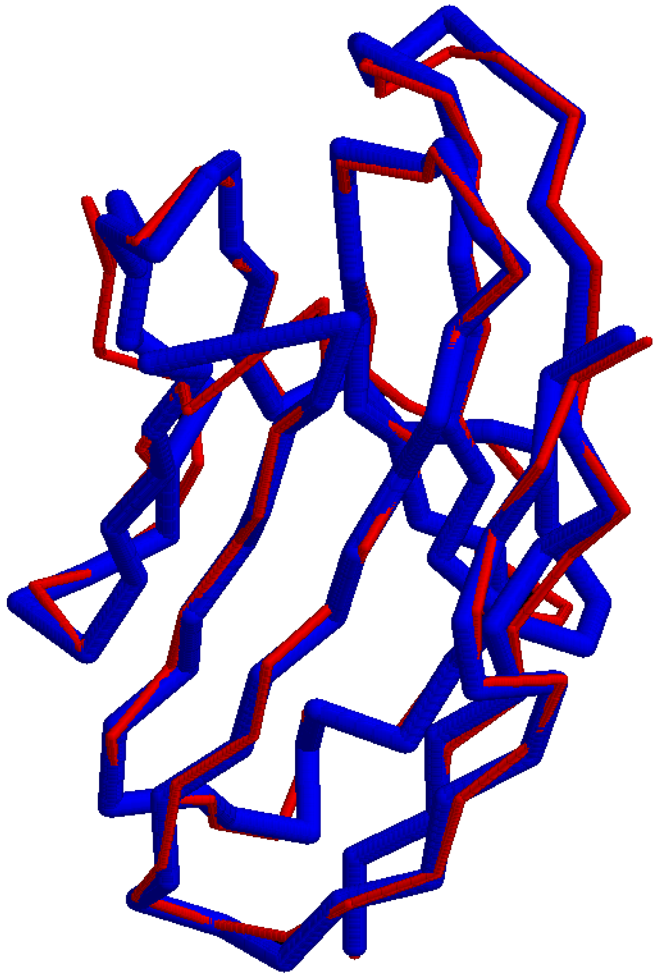
A complementary approach is to survey the world of possible peptides as sampled from protein structure data and subsequently test whether their geometric structure is mainly shaped by physical factors at the local level or at the global level of the molecule (Figure 2). The null hypothesis would be that any two small peptides with the same amino acid sequence, yet sampled from different non-homologous proteins, would not show similarity in their protein structure as measured by the TM score [31]. However, this test is based on the prior assumption that the TM score has a known level of significance for rejecting this null hypothesis, while this assumption may be met by the procedure as in other sections. Another assumption is on the availability of small peptide data. For a sequence of 9 amino acids, where there are 20 types of amino acids, a naive probability of finding any two randomly selected matching peptide pairs is 1 in 20 to the 9th power, which resolves to 1 in 520 billion pairs. However, the sampling of peptides with shorter lengths and fewer residues is expected to lead to finding identical pairs of peptides in a large database of protein structures. Moreover, this procedure depends on the reliability of the TM score metric as applied to cases with the above peptide length. If local factors of protein structure are in fact predictive of the structure of a small peptide, then it is possible to apply this knowledge to prediction of immunogenic peptides in Nature and therefore, the geometric distance between a known peptide and a predicted peptide is potentially quantifiable and meaningful.
4. Recognition of Peptides by T Cells
As described in the Introduction, predictive models of immunological peptides are dependent on position and chemical type of each amino acid: largely a consequence of their linear structure, a restriction on peptide length, and the molecular interactions that form an association with an MHC receptor (pMHC). Further, it has been reasonably established that the formation of the pMHC is dependent on the upstream pathways that restrict the length of these peptides [21]. However, this is descriptive of the peptide-MHC association [45], but not of the subsequent downstream pathway of T cell recognition [21,46]. However, it is known that the probability is very low for a peptide, as presented on the cell surface by an MHC receptor, to lead to an immune response. Therefore, the expectation is that most peptides, as presented on the cell surface by an MHC receptor, do not lead to an immune response.
As covered by Nielsen et al. [21], the problem is not in the robustness of models of pMHC binding, but in predicting that a peptide as presented on the cell surface is truly immunogenic [47]. For detection of these immunogenic peptides, a model must show high accuracy [48,49]. Given a model where the error rate from false negatives is set to a low value—~1 percent so that the number of potential epitopes is large and few candidates are absent—there is a concomitant increase in the false positive error rate for these predictions, leading to a limitation in detection of the set of true epitopes [21,50,51]. Given this rarity of immunogenicity in a sample of peptides, and the factors that lead to this rarity, modeling this phenomenon is limited [48], while the parameterization of the model is additionally hindered by the presence of unknown factors. With an informative data set, this is a kind of problem that is suitable for a deep learning approach, where the higher order features are captured by the model, including that of the atomic structure.
Gao and colleagues [52] developed a method and procedure in their article “Pan-Peptide Meta Learning for T cell receptor-antigen binding recognition”. It is based on meta learning principles and a neural Turing machine. In the case of zero-shot learning, where the potential for immunogenicity of peptides is not dependent on prior data during inference, the authors applied a procedure to validate their method in a T cell receptor–antigen dataset from a COVID-19 study [53]. Their method, PanPep [53], showed a model performance of ~0.7 (ROC-AUC analysis) [52,54]. They further showed that previous models do not discriminate better than a model of random chance. However, their model performance of ~0.7 was not evaluated as sufficiently robust, although this is a result for zero-shot learning, while they expect a higher predictiveness with the inclusion of prior data (few-shot learning). Additionally, PanPep [53] is capable of assessing the structural relationship between peptide and T cell receptor by simulation of an alanine substitutional analysis (an established technique in experimental biology) even though their data is solely based on sequence data [52], and the authors describe a “contribution score” for this relationship at each residue along the CDR3 region of the T cell receptor [52,55,56], a region of very high diversity [57,58] that is central to its pMHC interaction and any subsequent immune response. Therefore, this method is applicable for investigating a shift in the population of peptides as sampled from a pathogen and its impact on host immunity.
5. Model of T Cell Receptor Structure
5.1. Overview of the ImmuneBuilder Method
Since recognition of pathogenic peptides is dependent on T cells and their receptors, it is of interest to model the protein structure of these receptors. These models, such as AlphaFold [30], are expected to yield insight into peptide immunogenicity and emergent pathogen evolution.
While AlphaFold depends on a deep learning method for prediction of protein structure, it is not specifically adapted to the molecules of immunity. Therefore, Abanades and others developed ImmuneBuilder [59], a set of deep learning models specific to the hypervariable molecules of adaptive immunity. It includes a software component known as TCRBuilder2, which codes for a model to predict the protein structure of a T cell receptor. Further, the authors showed that their method is over 100× more performant than the AlphaFold approach. This higher performance in the generation of protein structure is also reflective of a high efficiency in the computation, so that this software is applicable for use in a computer workstation. Since TCRBuilder2 is specific to prediction of a restricted set of protein structures, it has removed any dependency on a prior that consists of multiple sequence alignments. This is in contrast to AlphaFold-Multimer [60], which is dependent on this since it is designed as a general model of protein structure.
The model weights of TCRBuilder2 are publicly available [59], and the model is based on a curated set of 704 T cell receptor variable domains [61]. Of these, a sample set of 50 records was used in a validation step and therefore excluded in the training of the model [59].
The RMSD metric [62], as described in an above section, is a measure for comparing the quality of predictions of protein structure, such as generated by TCRBuilder2 or AlphaFold-Multimer. In this case, the survey of methods showed similar levels of predictveness of the structure of T cell receptors [59]. For example, in the CDR (hypervariable complementarity-determining-regions) of the TCR alpha and beta chains, the mean RMSD metric values, as expressed in angstroms, are typically less than 2.0, while the values are nearer to 2.0 in the specific case of CDR3. In this case, the lower RMSD values indicate a closer correspondence between the structure of the prediction and that of the expectation for the protein structure, while a value of zero represents that a pair of proteins are identical.
In particular, CDR3 is an example of a highly hypervariable region, a distinct region as compared with the other regions of the T cell receptor. Therefore, in general, it is expected that the hypervariable regions require an increased sample size for yielding higher model predictiveness. This suggestion is based on achieving an expected level of robustness in modeling the more variable and widely distributed data source.
Interpretation of the RMSD values is dependent on knowledge of other factors at the molecular level, such as the sample size of amino acid residues. The TM score metric [31] has fewer assumptions to meet and is helpful in validating the values as generated by the RMSD metric. However, it is not uncommon to interpret a mean RMSD value of less than two angstroms as suggestive of structural similarity between two protein molecules. To further interpret the results of the TCRBuilder2 study, and for the purpose of disentangling the parameters of the model of protein structure, the authors examined measurements of error in the reconstruction of the six angles between the alpha and beta chains (ABangles) [63], the four torsion angles of the side chain (potentiality for peptide binding) [64], and solvent accessibility of amino acid residues [59]. Overall, their analysis of proteins by region is supportive of a robust interpretation of model performance against that of competing methods.
5.2. Usage of TCRBuilder2
The source code of ImmuneBuilder is available at GitHub [65]. The code includes instructions for an analysis that is based upon command line operation. Their repository also includes a Colab Notebook for testing TCRBuilder2. Furthermore, this software depends on several Python libraries which are in active development. A large number of library dependencies is common in projects that involve deep learning, so commonly used algorithms and code are relegated to a library for reuse. Since these dependencies are in active development, I made modifications to the Colab Notebook file for usage of TCRBuilder2 at Google Colab, such as modifications related to updates in the library dependencies [66]. The modified file of self-documenting code is shown in Appendix C.
The software generates an output file in PDB format that encodes the 3D structure of the protein. The RasMol software [67] can use an PDB formatted file to display this 3D structure, including in the form of a ribbon diagram of the arrangements of atoms in the molecule, but the export function to save a 3D image is not necessarily expected to work on recent versions of Microsoft Windows. In this case, the image may be captured by the simultaneous pressing of two keys on the keyboard, the “Alt” key and the “Print Screen” key, leading to a copy image operation. The captured image can then be inserted into a document by the simultaneous pressing of the “Ctrl” key and the “V” key, a paste image operation.
5.3. Verification of the TCRBuilder2 Model
As described below, the TCRBuilder2 can generate a 3D protein structure from the input consisting of protein sequences that correspond to the two TCR polypeptide chains, such as the complement of alpha and beta chains. In the following example, the input is a protein complex from the RCSB database [68]: PDB record 5d2l (rcsb.org/structure/5d2l), which includes an empirically determined protein structure, a potential benchmark for measuring the quality of the protein prediction by TCRBuilder2. The empirical data for 5d2l are exportable as a PDB-formatted file. This data file appears to correspond to an empirical analysis of a quaternary crystal structure of a protein. To further examine their empirical analysis, the PDB record was referenced to find any literature associated with the record. An article is associated and entitled “Structural Basis for Clonal Diversity of the Public T Cell Response to a Dominant Human Cytomegalovirus Epitope” [69]. It has the following relevant details:
“The corresponding r.m.s.d. for the four C7·NLV·HLA-A2 complexes ranged from 0.50 to 0.83 Å. Based on these close similarities, the following descriptions of TCR-pMHC interactions apply to all complex molecules in the asymmetric unit of the C25·NLV·HLA-A2 or C7·NLV·HLA-A2 crystal”.
“Three complex molecules in the asymmetric unit were located first; the fourth was found according to non-crystallographic symmetry”.
To validate the above statements, a method is described below to confirm that the record 5d2l is composed of four empirically derived samples corresponding to the same protein complex. First, the empirical data (in this case, PDB formatted) are processed for collating the alpha and beta chains of the TCR receptor, along with their amino acid sequences. Comparisons of the data samples by chain type show that they are identical or nearly identical at the amino acid residue level. Therefore, the data are expected to truly contain four separate models that are based on four empirical samples of the crystallization of a single protein complex. Third, there is a REMARK section in the file with descriptions of 4 BIOMOLECULE(S).
The PDB formatted file of record 5d2l is annotated with information on the individual polypeptide chains. For this case, the relevant data fields are identified by the prefix name COMPND:
COMPND 12 MOL_ID: 3
COMPND 13 MOLECULE: C7 TCR ALPHA CHAIN
COMPND 14 CHAIN: I, K, O, E
COMPND 16 MOL_ID: 4
COMPND 17 MOLECULE: C7 TCR BETA CHAIN
COMPND 18 CHAIN: J, L, P, F
The alpha and beta chains of the TCR are annotated with letter assignments that correspond to the four empirical models. The alpha chain is represented in the data file as I, K, O, and E; likewise, the beta chain is represented as J, L, P, and F. In the file, there are also fields that list the amino acid residue sequence of each of these polypeptide chains. This data can be extracted by searching for the data fields containing a prefix of SEQRES and a letter that signifies the polypeptide chain of interest. For viewing these amino acid sequences and their residue similarity, a sequence alignment software is an appropriate tool, such as ClustalW [70]. An amino acid sequence alignment of the TCR beta chain is shown in Figure 3 (confirming the identity of the four beta chains in the 5d2l data record).
In this record, the corresponding pairs of TCR alpha and beta chains are shown by viewing the data fields with a prefix name BIOMOLECULE, revealing that polypeptide chains I and J are of the same sample and therefore correspond to the alpha and beta chains of the TCR, respectively. These PDB formatted files can then be used to create PDB-formatted files specific to each of the chains I and J. The predictions by TCRBuilder2 are presented in PDB format, so comparisons are possible between it and the 3D protein structure stored in the PDB database. Next, the PDB data fields that are prefixed with the label name ATOM of the TCR alpha chain are aligned (by visual inspection) and then trimmed so that the amino acid residues of the sequences are comparable and orthologous between the PDB record and that generated by TCRBuilder2. This procedure was repeated for the beta chain. The goal is to have a comparison between data that represents aligned amino acid residues, where each residue is orthologous between the comparisons. Last, the index value of the amino acid residues (data fields for residues have the prefix name ATOM) was reset as described in another section on use of the TM score metric.
Next, TM score is used to compute the TM score values [31]. The command line below is an example of this procedure. The “seq” parameter may be appended to align the sequence data via the software, but this practice is not foolproof, and—if used—the sequences should be verified by inspection of the output file. Instead, it may be preferable to construct the alignments beforehand.
| tmscore 5d2l_prediction_A.pdb 5d2l_ChainA-I.pdb > 5d2l_A_RMSD.out tmscore 5d2l_prediction_B.pdb 5d2l_ChainB-J.pdb > 5d2l_B_RMSD.out |
The output of the TCR alpha chain comparison (the first line above) reports an TM score value of 0.9539 across 98 residues. For the beta chain, the TM score value is 0.9426 across 110 residues. This verifies that TCRBuilder2 is constructing models of protein structure that closely resemble the empirical models in the PDB record.
Furthermore, TM score has an option to compute the superposition data for viewing protein structure similarity (the “seq” parameter may be appended, if needed):
| tmscore 5d2l_prediction_A.pdb 5d2l_ChainA-I.pdb -o 5d2l_A_SUP tmscore 5d2l_prediction_B.pdb 5d2l_ChainB-J.pdb -o 5d2l_B_SUP |
5.4. Comments on TCR Modeling by Deep Learning
Even though ImmuneBuilder is competitive with the more generalized model of Alphafold-Multimer, it is of interest to expand deep learning models that are specific to one that is applicable to a greater set of problems. For example, generalization is preferred to achieve a broader parameterization of 3D protein structures and for capturing the rarer patterns of atomic arrangements. However, at this time, the specificness of the ImmuneBuilder approach is reasonable since it shows very good performance during the inference and generation of 3D protein structures. Another goal of interest is in expanding the collection of TCR data so that a model has the potential to sample data more broadly. Collectively, these goals, and others, contribute to increased performance in these deep learning approaches and converge on the possibility of meaningful analysis of the shift in protein structure of an T cell receptor that is associated with changes in peptide binding and, therefore gain an eventual insight into the proximate mechanisms of adaptive immunity at the host population level.
The field of deep learning is expanding on techniques with applicability to TCR modeling, such as in the use of a large language model to “perform evolutionary optimization over reward code” and the use of “the resulting rewards... to acquire complex skills via reinforcement learning” [71]. This approach refers to an example that was applied to the field of robotics, but the methodology is applicable to other tasks and in automation of trial-and-error experimentation, such as in an informatics pipeline for identification of immunogenic peptides and their putative association with an MHC receptor and subsequently its downstream effects on immune surveillance by the T cell receptor repertoire. This type of automatability in deep learning is akin to an outer loop that has control over an inner loop, which codes for the world of possible predictions, so the overall system is recursive in its operation and has the potential for planning and application to the practice of experimentation. This kind of perspective and approach is seen in deep learning by the intelligent processing of input and verification methods for assessing model output. Related approaches that apply to immunogenetics are expanded upon below (Section 7).
6. Molecular Signature of Peptide Immunogenicity
With a sufficiently large and broad sampling of data, the deep learning approaches are generally applicable in modeling the immunological pathways, particularly where traditional approaches, based on a set of fewer interpretable parameters, are inadequate. More specifically, since the small peptides are a major determinant of adaptive immunity in the jawed vertebrates, it is essential to collect a broad set of empirical data to represent and parameterize the elements of immunogenicity [21]. Without these models, there is an expectation of low predictiveness for any model of pathogen evolution, and, therefore, the practitioners of this science may tend toward the excesses of reductionism [72] and misperceptions about the true model, which relates to the inner workings of adaptive immunity.
The above is a view based on making predictions about immunogenic peptides as sampled and derived from a pathogen of interest. However, another approach is to compare the evolution of a specific pathogen against generated data from the highly accurate peptide–MHC binding models [21,45]. This suggestion is for simulation of changes in the genome of the pathogen and subsequent identification of the changes that putatively weaken the binding association between peptide and MHC receptor. The distribution of amino acid substitutions in these simulations may be compared against prior knowledge of the evolution of a pathogen and its response to host immunity. The comparisons would provide insight into the numbers and types of amino acid changes that are characteristic of an evolutionary response of a pathogen, including a predictiveness on novel variants and their potential for evasion of host immunity. The assumption of this comparative approach is that the peptide-MHC association is a vulnerable pathway to the evolution of a successful pathogen. Another potential strategy is for the pathogen to target the host pathway that cleaves and forms peptides prior to an association with an MHC receptor. Third, a pathogen may evolve so the resultant peptides in the host are no longer identified as immunogenic by the downstream pathways of host immunity, although it is presumed that all three pathways are potential targets by the pathogen in its evolutionary search for success in the host-pathogen interaction. However, the relative utilization of each of these strategies by pathogens is not well understood.
This approach is confounded by the feasibility of identification of the specific amino acid substitutions that are associated with an evolutionary response by a pathogen to a host, as substitutions may be caused by other factors, and the genomic signature of the host response may have been subsequently erased by evolutionary changes. It is possible to discriminate between these evolutionary changes based on their association with the forces of natural selection. For example, nucleotide substitution methodology is available to predict when a genomic region shows a signature of positive selection, and the signature is measured by comparison of the rates of nonsynonymous to synonymous substitutions (Figure 6) [73]. A nonsynonymous change is specifically defined as a nucleotide change that leads to an amino acid change, while a synonymous change is a silent substitution at the amino acid level. This approach is limited by a confidence in the measurement of the rate of synonymous change, such as cases in which nucleotide sites have undergone a high number of synonymous changes and the corresponding error rate is high. The regions which are confidently identified as having undergone evolution by positive selection are ideal candidates for further study on the evolutionary response of a pathogen to a host.
Last, the immune response by a host is not dictated by any single peptide and T cell receptor type, but by a process based on combinations of different peptides and T cell receptor types [74]. This population level perspective of peptides and their associations with T cell receptors is illustrative of an applicable approach to a robust modeling of the host immune response to a pathogen at the level of the individual. It further conforms to the mathematics of a sampling process, so the immunological system is, on average, reacting to a true molecular signal of a pathogen and not a spurious sample based on a low sample size of signals at the molecular level. It also dampens the error that results from a false signaling of the presence of a pathogen, as in the cross-reactivity of the MHC receptor to non-pathogenic peptides [10]. Moreover, the biological systems, as often documented in the science of animal development and a testament to the forces of evolution [75,76], are an interplay between the intrinsic error of biological pathways and compensatory processes that regulate and canalize for a desired outcome. The robust sampling process by the host immune system is an example of this kind of regulation, so a costly immune response to non-pathogens is minimized, and detection of a true pathogenic infection is maximized. An error in the biological pathways remains, but the mere evolutionary history of vertebrates [77] is supportive that this evolved system is robust and that their populations are competitive in an evolutionary context.
7. Deep Learning and Immunogenetics
7.1. Deep Learning Architectures
Deep learning is applicable to the biological sciences where the data are representable by a sequence of tokens, such as a nucleotide sequence of a gene or the linear encoding of the structure of a protein [30,78,79,80]. Ideally, the architecture of a deep learning model is provided with an adequately large data set for use in its training procedure, which then leads to some capacity for generating predictions, such as in the case of ESMFold [81], a transformer-based model that robustly learns the higher order structural elements of proteins from training on prior data. Moreover, the transformer is an ideal architecture for use across the natural sciences since it is frequently tested during use by engineers and scientists. For the immunological pathways, there is more than one approach in the use of the transformer.
In the case of a pathogen that is genetically responding to a host, an approach to modeling this phenomenon is by collecting genetic and environmental data, including the interactions between pathogen and host. The sequence-based transformer model is adaptable for learning from this kind of data set and some subsequent capability in making predictions on the evolutionary response by the pathogen. However, the data requirements are high for robust predictiveness on the evolution of a pathogen.
Another method, as described in an above section, is to focus on a part of an immunological pathway, such as the probability of the formation of a protein complex between MHC and small peptides, given this association is robustly modeled. In this case, deep reinforcement learning is also applicable, particularly where both the method of deep learning and of reinforcement learning are applied [82,83]. In a reinforcement learning method, an agent learns a policy by taking an action and receiving a reward. This is a useful approach to highly complex biological systems, where there is a dependence on a large space of possible states and quantifiable parameters as seen in the areas of genetics and cellular biology. In the case of the evolution of a pathogen, it is possible to train a model in which the genetic sequence of the pathogen is the agent, genetic substitution is the action, and the MHC-peptide model determines the reward for any genetic modification [84].
A third approach is to rely on advanced prompting methods in deep learning [85]. A diversity of deep learning models can serve as modules where the connections between them are written in the form of computer code, such as in Python. One module may be designated to run a program for computing the probability of the formation of an MHC–peptide complex. Another module could generate the sequence data for input, while a third module could serve as a database that receives, processes, and stores the results. This chain of models and modules are functioning as an informatics pipeline of programs and data [86]. It is both an extensible and kind of recursive learning process, where each module has a unique role, including in the form of decision-making or the running of an external tool or program [87]. A mechanism to connect these modules is by use of Python code, a computer language adapted for modifying and testing new procedures in an informatics pipeline. The code serves as an essential “glue” that binds the modules together. This approach also allows for integration between local and remotely accessible models, an efficient scheme where each model is specific to a purpose and computing resources are distributed across geographical locations.
The modular approach to deep learning is somewhat similar to the mixture of experts model (MoE) in deep learning [88]. MoE is expected to depend on a gating neural network that routes data among the other networks, where each network learns a specialized task or tasks. An advantage of the modular approach is that models can be assigned to evaluate and validate the output from the other modules in a process that allows for an increase in interpretability of the system of modules. Overall, the approach offers a flexible methodology for recursive learning and a path to achieving a meta-learning approach.
7.2. Meta-Learning Systems
Recent advances in large language models have resulted in better predictiveness and interpretability [89,90]. These advances are dependent on the transformer architecture [78,91], hardware for large scale parallel computing [92], and extensive collection and curation of data. The curated data is first transformed to a tokenized format, which, in this case, is words and subwords, while the transformer is the engine for discovery of the associations in a sequence of tokens and leads to a model that predicts the next token based on a sequence of prior tokens [80]. These large language models are often fine-tuned for interactions in the form of common dialog [93]. Further, these models have been extended to include data for providing assistance in the practice of natural science [94]. However, these models have shown a deficit in the use of higher-order concepts, a probable reference to general reasoning, although prompting methods have had success in mitigating these shortcomings [95,96,97]. This is the gap between a statistical model that predicts the next word and any robust process of general reasoning [98]. A capability of general reasoning is expected to lead to models with a greater automation of scientific practice, notwithstanding that deep learning models have already contributed to knowledge across the natural sciences [30,59,99].
The automation of a deep learning system may be referred to as meta-learning, an iterative and recursive approach to validating and improving predictions. This kind of technique has been applied to board games [100], where it is possible to assign a policy and value function so that the system can plan and identify the best action for maximizing a reward that is dependent on the subsequent set of states of the game board. This model is ideal in modeling the processes of general reasoning, but in a language model, the rewards are not as easily quantified. However, prompting methods have led to a capability of general reasoning in the use of large language models [96,97]. These methods also depend on strategies, such as reduction of a complex problem to a set of tractable subproblems, along with a system for validation of a response.
This deep meta-learning approach is akin to a compression of the total states possible for a given subproblem, so the dimensionality of the overall problem is lowered. This is expected from fundamental theory [101] and studies in neuroscience [102,103]. A compression of information is expected to lead to better feature detection for the goal of robust construction of the higher-order associations as mirrored in the act of conceptualization and higher cognition. The prompting methods cited earlier are examples of iteratively querying the model to constrain and compress the pathways in a search for the best possible output. Therefore, in the cases where this approach is required and successful, then the model is capable of finding the correct answer, given correctness is possible, but without this approach, the dimensionality of the search space may extend beyond what is computationally feasible. Various prompting methods also can compress the search space by transforming queries into a lower dimensional form (pseudocode) [97,104], which may lead to a value function that is applicable for a particular task [105].
It seems reasonable that large language models can add to their capacity for general reasoning by a reduction of a problem to a set of subproblems, reduction of statements to any lower dimensional format, and the ability to assign a reward to the model’s successes. A related optimization is that of data quality and structure enhanced by the use of what is referred to as synthetic data [106]. Altogether, these approaches involve data compression, validation of output, and automated iteration in the search for reliable results [107] within a meta-learning framework.
7.3. Interpolation and Extrapolation in Deep Learning
Another problem in deep learning is whether learning from high dimensional data is dependent on interpolation or extrapolation [108]. LeCun and colleagues define these terms within a geometrical framework and subsequently infer that high dimensional data is frequently learned by extrapolation in the case of “state-of-the-art algorithms” rather than a stricter dependence on interpolation [108]. Therefore, in the case of problems in biology, it may be inferred that deep learning architectures are capable of learning from data that exceeds that expected if a model is only capable of interpolation.
The capability for these models to generalize is seen in the processing of natural language. It is possible to fine-tune a large pre-trained model for a specific task when the prior training step has achieved a capability for generalization across the space of all possible tasks [109]. This is a relevant idea with applicability to peptide structure and problems in immunology. These are systems of high dimensionality, so the use of “big data” approaches that incorporate data from disparate sources is informative. For example, analysis of the binding between T cell receptor and peptide are a product of atomic interactions, and, therefore, a general model of protein structure is expected to increase the applicability of a deep learning model to molecules of the immune system. This approach would reduce the reliance on any deficit of data in modeling the structures of molecules of immunity, such as in the modeling of the TCR–peptide–MHC interactions that extends beyond the role of the CDR3 beta chain of the T cell receptor [48,52] and inclusion of priors that parameterize the MHC receptor by type [22,52].
8. Conclusions
Small peptides are crucial to the functions of the immunological pathways in vertebrates. Their dynamical interactions with other molecules occur in three-dimensional space, but, in the case of its association with the MHC Class 1 receptor, the linear peptide may be modeled by amino acid position and property. Otherwise, peptide structure at all scales is crucial for an accurate modeling of immunological pathways, such as in the detection of pathogenic peptides by the pathway involving the pMHC and its surveillance by a T cell receptor. Although protein sequence and structural data are ideally plentiful, particularly in application for deep learning modeling, there are other approaches to modeling these systems, such as in isolating the tractable pathways, where one example is in the formation of the peptide–MHC complex. Since these pathways are complex systems, high in dimensionality, and not well understood, it is worthwhile to employ deep learning models and related machine learning architectures [52] for advancement in modeling the major pathways of immunobiology and for prediction of the evolution of pathogens in response to a vertebrate host.
Lastly, general models of immunobiology should incorporate a population level perspective and avoid a narrow viewpoint that merely centers on the atomic arrangements. This is a suggestion to view the system at the scale of a population. The peptides of a pathogen that are generated by host immune processes are essentially a population of potentially immunogenic peptides. An evolution of the pathogen can be considered a “shift” [110] in the population of peptides. This shift in this population may or may not correspond to a change in immunogenicity in the overall peptide population. Furthermore, the immunogenicity of peptides is largely a function of its association with an MHC receptor and detection by a T cell receptor and can lead to a downstream immune response in the host. The collection of these singular responses at the cellular level are a population of events, and a host immune response is dependent on the occurrence of a sufficiently large number of events. Where the pathogen is in interaction with the adaptive immune system of a vertebrate host, it responds to these events by evolution, presumably by natural selection. This evolution is also a population-level phenomenon. Likewise, at the cellular level, the adaptive immune system of a host is or has undergone genetic changes by recombinational and mutational processes, leading to novel populations of cells that function in this system [111,112]. Both the evolution of the pathogen and the adaptation for immunity in the host population, are important elements in modeling the spatiotemporal dynamics of the pathogen–host interaction.
Funding
This research received no external funding.
Institutional Review Board Statement
Not applicable.
Informed Consent Statement
Not applicable.
Data Availability Statement
Data are contained within the article, a trusted repository, and at publicly available sites.
Conflicts of Interest
The author declares no conflicts of interest.
Appendix A
Appendix A.1. Peptide Structure Data
Predictions of protein structure in PDB formatted files are available across the many divisions of cellular life: https://alphafold.ebi.ac.uk/download (accessed on 10 March 2024) (Figure A1). These files are stored as an archival file type (.tar), so the “tar” program is useful in extracting the set of files contained within the greater archival file. The archive file sizes are generally large in this case, so an alternative to a conventional web-based retrieval is to use the “curl” program at the command line, which is capable of resuming from a failure in the file transfer process as can occur from network connection loss. An example is below for obtaining a relevant sample of mouse data:
| curl –O https://ftp.ebi.ac.uk/pub/databases/alphafold/latest/UP000000589_10090_MOUSE_v4.tar (accessed on 10 March 2024) |
The above archive file (tar file format) has both PDB and mmCIF formatted file types per protein. A command line is shown below for restricting the file extraction process to the PDB file type:
| tar –xvf UP000000589_10090_MOUSE_v4.tar *.pdb.gz |
As follows from use of the “gz” file extension in the above example, each PDB formatted file had been compressed to a smaller file size in a binary format (gzip file format), so a decompression operation would lead to a plain text file with the PDB protein structure data. To decompress these files in a single operation, the “gzip” program is commonly used:
| gzip –d *.gz |
Since the tar-based archive file itself is not compressed, but the data files contained within the archive are compressed, the unarchival operation to extract these files to a directory will use disk space similar to that of the original size of the archive file. However, decompression of the individual compressed data files (gzip file format) will occupy a much larger space on the storage device because each of these data files is expected to uncompress to four times of its original file size. Therefore, if the uncompressed data files of interest occupy four gigabytes of disk storage, then the decompression operation is expected to result in the use of 16 gigabytes of disk space. Since this example corresponds to a single organism and its protein structure data files, the disk storage requirement is consistent with the capabilities of a desktop computer. However, extending a study to other organisms, or inclusion of protein structure prediction data across the Swiss-Prot database, would lead to a very large use of disk space. In this case, another requisite is that the file system show robustness in the handling of a very large number of data files, since the above method can generate from a few thousand to greater than a million files on the disk.
Figure A1.
Sample of a PDB formatted file that describes the 3d atomic structure of a hemoglobin protein from an avian species (1HV4) [43]. This format is described online: https://www.cgl.ucsf.edu/chimera/docs/UsersGuide/tutorials/pdbintro.html (accessed on 10 March 2024). For this sample, the description of each row is in the first, fourth, fifth, and last columns. The first column is a key name for the layout of the row and its data. In this case, it is the key word ATOM which refers to the data type in the row. In this case, it is atomic level data. The last column is a one-letter abbreviation for the chemical element that corresponds to the atomic level data in the row. Lastly, the fourth column lists the three-letter abbreviation of the amino acid molecule that is the parent of the atomic element, and the fifth column lists the identifying name of the protein chain. The seventh, eighth, and ninth rows correspond to the X, Y, and Z coordinates of the atom, respectively, and its position in three-dimensional space.

Appendix A.2. Parsing the PDB Data Files
The PDB formatted data files are expected to conform to the standardized format as described at the site below:
| https://www.cgl.ucsf.edu/chimera/docs/UsersGuide/tutorials/pdbintro.html (accessed on 10 March 2024) |
As a rule, each PDB formatted data file can contain more than one model per protein structure. It may also describe more than one protein chain per model. To help enumerate these features, in Appendix B there is Python computer code for parsing the PDB data file by these both these features, which then prints out the names of the models and polypeptide chains of the protein [42].
Other code samples are at a GitHub web site for processing PDB data files [42], including a template for splitting a PDB data file into multiple data files, where each split file represents a window of nine amino acid residues. For this case, the window is shifted by one residue per newly created file, so the procedure is equivalent to sliding a window along the sequence of amino acid residues of a protein and writing that data to a file that corresponds to the window of nine amino acids and the associated protein structure data. However, this procedure leads to disk space usage that is orders of magnitude greater than the disk space occupied by the original PDB data files. The count of files likewise increases by the same factor, while the Python code is not a performant language in processing these kinds of file operations, given the expectation it is processing the code in a single thread, and furthermore, the code in this example is not necessarily translated by the Python code interpreter to a form of highly efficient machine code, as in a low-level programming language which is adapted for efficiency in the processing of machine instructions.
Appendix A.3. Format of Data Files for TM Score
Appendix B has a second code sample. In this case, it resets the amino acid residue number—an index of each PDB data file—since by default, the TM score expects that the sequence of residues in each of the two input data files are beginning with the same index numbering scheme.
Appendix B
This section has two samples of Python code for processing PDB formatted data files (note that this code is formatted for a publication standard that does not retain the original indentation scheme or the original usage of special characters). These files are expected to conform to the standardized format as described at the following web site:
| https://www.cgl.ucsf.edu/chimera/docs/UsersGuide/tutorials/pdbintro.html (accessed on 10 March 2024) |
Each PDB data file can describe more than one three-dimensional model of the one or more polypeptide chains of a protein and its structure. Below is code for parsing each PDB data file by these two features, which then displays the names of the model and the amino acid chains of the protein [42]:
| import glob from Bio.PDB.PDBParser import PDBParser # assign functions parser = PDBParser() # input file for file in glob.glob(‘./*.pdb’): print(“file: “, file) # retrieve PDB structure structure = parser.get_structure(file, file) # iterate over models and chains in file for model in structure: print(“model: “, model) for chain in model: print(“chain: “, chain) |
Below is the second code sample. In this case, the procedure resets the amino acid residue number, an index, of each PDB data file, since by default TM score expects that the amino acid sequences in the input data files are annotated with the same index-based numbering scheme:
| import os directory = ‘C:/Peptide3d/data’ files = os.listdir(directory) for file in files: if file.endswith(‘pdb’): print(file) pdb_file = file with open(pdb_file, ‘r’) as f: lines = f.readlines() current_residue = None start_residue = 1 current_residue_number = start_residue − 1 for i, line in enumerate(lines): if line.startswith(‘ATOM’): residue = line[22:26] if residue != current_residue: current_residue = residue current_residue_number += 1 lines[i] = line[:22] + str(current_residue_number).rjust(4) \ + line[26:] if line.startswith(‘TER’): residue = line[22:26] if residue != current_residue: current_residue = residue lines[i] = line[:22] + \ str(current_residue_number).rjust(4) + line[26:] with open(pdb_file, ‘w’) as f: f.writelines(lines) |
Appendix C
The Python code below is in the form of a Colab Notebook. It is modified source code to access TCRBuilder2 and is available at a GitHub site [42]. The code is organized as two separate blocks of code.
- Step 1. Install TCRBuilder2 library dependencies:
| # Edit sequence_1, sequence_2, filename—the input data for prediction of 3d structure # The Colab runtime may report a crash from an expected restart during installation of a library # Comment out this line to enable verbose output %%capture !pip install ImmuneBuilder # use Python installer to install ImmuneBuilder (TCRBuilder2) !pip install -q condacolab # google colab-compatible access to conda import condacolab, sys # import modules to access their functions condacolab.install_mambaforge() # use of mamba to install conda modules !mamba install openmm # install openmm (toolkit for molecular simulation; refine prediction) !mamba install pdbfixer # install pdbfixer (fix problems in PDB formatted files) !conda install -y -c bioconda anarci # install anarci module from bioconda distribution |
- Step 2. Install TCRBuilder2 and run the model:
| # Delete and restart Colab runtime to avoid unexpected errors in the following code # Comment out this line to enable verbose output %%capture !pip install -q ImmuneBuilder # use Python installer to install ImmuneBuilder (TCRBuilder2) protein_type = “TCR” from anarci import number # github.com/oxpig/ANARCI; aligns sequence to canonical protein from ImmuneBuilder import TCRBuilder2 # prediction of 3d structure # Select model predictor = TCRBuilder2() # “TCRBuilder2” or “ABodyBuilder2” model # Inspect that TCR sequences are annotated as TCR alpha and beta chains # Below is sequence data from www.rcsb.org/structure/5d2l (accessed on 10 March 2024) sequence_1 = ‘MILNVEQSPQSLHVQEGDSTNFTCSFPSSNFYALHWYRWETAKSP\ EALFVMTLNGDEKKKGRISATLNTKEGYSYLYIKGSQPEDSATYLCAFITGNQFYF\ GTGTSLTVIPNIQNPDPAVYQLRDSKSSDKSVCLFTDFDSQTNVSQSKDSDVYITDK\ CVLDMRSMDFKSNSAVAWSNKSDFACANAFNNSIIPEDTFFPSPESS’ sequence_2 = ‘MGAGVSQSPSNKVTEKGKDVELRCDPISGHTALYWYRQRLGQGLE\ FLIYFQGNSAPDKSGLPSDRFSAERTGESVSTLTIQRTQQEDSAVYLCASSQTQLWET\ QYFGPGTRLLVLEDLKNVFPPEVAVFEPSEAEISHTQKATLVCLATGFYPDHVELSW\ WVNGKEVHSGVCTDPQPLKEQPALNDSRYALSSRLRVSATFWQNPRNHFRCQVQF\ YGLSENDEWTQDRAKPVTQIVSAEAWGRAD’ sequence_1 = ““.join(sequence_1.split()) # Remove whitespace sequence_2 = ““.join(sequence_2.split()) # Remove whitespace filename = ‘output.pdb’ # output file name as PDB formatted file (viewable in RasMol) # Anarci will reject the sequence if it is not an expected match to the immunoprotein _, chain1 = number(sequence_1) # set key for chain 1 to input sequence _, chain2 = number(sequence_2) # set key for chain 2 to input sequence input = dict() # initialize hash table of key-value pairs if chain1: input[chain1] = sequence_1 # add sequence value to key for hash table if chain2: input[chain2] = sequence_2 # add sequence value to key for hash table predictor.predict(input).save(filename) # run 3d prediction of TCR, save to file |
References
- Wieczorek, M.; Abualrous, E.T.; Sticht, J.; Álvaro-Benito, M.; Stolzenberg, S.; Noé, F.; Freund, C. Major Histocompatibility Complex (MHC) Class I and MHC Class II Proteins: Conformational Plasticity in Antigen Presentation. Front. Immunol. 2017, 8, 292. [Google Scholar] [CrossRef] [PubMed]
- Dhatchinamoorthy, K.; Colbert, J.D.; Rock, K.L. Cancer Immune Evasion through Loss of MHC Class I Antigen Presentation. Front. Immunol. 2021, 12, 636568. [Google Scholar] [CrossRef] [PubMed]
- Peters, B.; Nielsen, M.; Sette, A. T Cell Epitope Predictions. Annu. Rev. Immunol. 2020, 38, 123–145. [Google Scholar] [CrossRef] [PubMed]
- Engelhard, V.H. Structure of peptides associated with MHC class I molecules. Curr. Opin. Immunol. 1994, 6, 13–23. [Google Scholar] [CrossRef] [PubMed]
- Davis, M.M.; Bjorkman, P.J. T-cell antigen receptor genes and T-cell recognition. Nature 1988, 335, 744. [Google Scholar] [CrossRef]
- Serwold, T.; Gonzalez, F.; Kim, J.; Jacob, R.; Shastri, N. ERAAP customizes peptides for MHC class I molecules in the endoplasmic reticulum. Nature 2002, 419, 480–483. [Google Scholar] [CrossRef] [PubMed]
- Clevers, H. The T Cell Receptor/Cd3 Complex: A Dynamic Protein Ensemble. Annu. Rev. Immunol. 1988, 6, 629–662. [Google Scholar] [CrossRef]
- Theofilopoulos, A.N.; Kono, D.H.; Baccala, R. The multiple pathways to autoimmunity. Nat. Immunol. 2017, 18, 716–724. [Google Scholar] [CrossRef]
- Uemura, Y.; Senju, S.; Maenaka, K.; Iwai, L.K.; Fujii, S.; Tabata, H.; Tsukamoto, H.; Hirata, S.; Chen, Y.Z.; Nishimura, Y.; et al. Systematic Analysis of the Combinatorial Nature of Epitopes Recognized by TCR Leads to Identification of Mimicry Epitopes for Glutamic Acid Decarboxylase 65-Specific TCRs. J. Immunol. 2003, 170, 947–960. [Google Scholar] [CrossRef]
- Borrman, T.; Pierce, B.G.; Vreven, T.; Baker, B.M.; Weng, Z. High-throughput modeling and scoring of TCR-pMHC complexes to predict cross-reactive peptides. Bioinformatics 2020, 36, 5377–5385. [Google Scholar] [CrossRef]
- Prinz, J.C. Immunogenic self-peptides—The great unknowns in autoimmunity: Identifying T-cell epitopes driving the autoimmune response in autoimmune diseases. Front. Immunol. 2023, 13, 1097871. [Google Scholar] [CrossRef] [PubMed]
- Yanagi, Y.; Yoshikai, Y.; Leggett, K.; Clark, S.P.; Aleksander, I.; Mak, T.W. A human T cell-specific cDNA clone encodes a protein having extensive homology to immunoglobulin chains. Nature 1984, 308, 145–149. [Google Scholar] [CrossRef] [PubMed]
- Hedrick, S.M.; Cohen, D.I.; Nielsen, E.A.; Davis, M.M. Isolation of cDNA clones encoding T cell-specific membrane-associated proteins. Nature 1984, 308, 149–153. [Google Scholar] [CrossRef] [PubMed]
- Yang, Q.; Bell, J.J.; Bhandoola, A. T-cell lineage determination. Immunol. Rev. 2010, 238, 12–22. [Google Scholar] [CrossRef] [PubMed]
- Nikolich-Žugich, J.; Slifka, M.K.; Messaoudi, I. The many important facets of T-cell repertoire diversity. Nat. Rev. Immunol. 2004, 4, 123–132. [Google Scholar] [CrossRef] [PubMed]
- Ashby, K.M.; Hogquist, K.A. A guide to thymic selection of T cells. Nat. Rev. Immunol. 2023, 23, 697. [Google Scholar] [CrossRef] [PubMed]
- George, J.T.; Kessler, D.A.; Levine, H. Effects of thymic selection on T cell recognition of foreign and tumor antigenic peptides. Proc. Natl. Acad. Sci USA 2017, 114, E7875–E7881. [Google Scholar] [CrossRef] [PubMed]
- Smith, D.A.; Germolec, D.R. Introduction to Immunology and Autoimmunity. Environ. Health Perspect. 1999, 107, 661. [Google Scholar]
- Klein, J.; Figueroa, F. Evolution of the major histocompatibility complex. Crit. Rev. Immunol. 1986, 6, 295–386. [Google Scholar]
- Germain, R.N. MHC-dependent antigen processing and peptide presentation: Providing ligands for T lymphocyte activation. Cell 1994, 76, 287–299. [Google Scholar] [CrossRef]
- Nielsen, M.; Andreatta, M.; Peters, B.; Buus, S. Immunoinformatics: Predicting Peptide–MHC Binding. Annu. Rev. Biomed. Data Sci. 2020, 3, 191–215. [Google Scholar] [CrossRef] [PubMed]
- Radwan, J.; Babik, W.; Kaufman, J.; Lenz, T.L.; Winternitz, J. Advances in the Evolutionary Understanding of MHC Polymorphism. Trends Genet. 2020, 36, 298–311. [Google Scholar] [CrossRef] [PubMed]
- Jorde, L.B. Genetic variation and human evolution. Am. Soc. Hum. Genet. 2003, 7, 28–33. [Google Scholar]
- Bjorkman, P.J.; Saper, M.A.; Samraoui, B.; Bennett, W.S.; Strominger, J.L.; Wiley, D.C. Structure of the human class I histocompatibility antigen, HLA-A2. Nature 1987, 329, 506–512. [Google Scholar] [CrossRef] [PubMed]
- Antunes, D.A.; Devaurs, D.; Moll, M.; Lizée, G.; Kavraki, L.E. General Prediction of Peptide-MHC Binding Modes Using Incremental Docking: A Proof of Concept. Sci. Rep. 2018, 8, 4327. [Google Scholar] [CrossRef]
- Mei, S.; Li, F.; Leier, A.; Marquez-Lago, T.T.; Giam, K.; Croft, N.P.; Akutsu, T.; Smith, A.I.; Li, J.; Rossjohn, J.; et al. A comprehensive review and performance evaluation of bioinformatics tools for HLA class I peptide-binding prediction. Brief. Bioinform. 2020, 21, 1119–1135. [Google Scholar] [CrossRef] [PubMed]
- Sohail, M.S.; Ahmed, S.F.; Quadeer, A.A.; McKay, M.R. In silico T cell epitope identification for SARS-CoV-2: Progress and perspectives. Adv. Drug Deliv. Rev. 2021, 171, 29–47. [Google Scholar] [CrossRef]
- Raoufi, E.; Hemmati, M.; Eftekhari, S.; Khaksaran, K.; Mahmodi, Z.; Farajollahi, M.M.; Mohsenzadegan, M. Epitope Prediction by Novel Immunoinformatics Approach: A State-of-the-art Review. Int. J. Pept. Res. Ther. 2019, 26, 1155–1163. [Google Scholar] [CrossRef]
- Bradley, P. Structure-based prediction of T cell receptor:peptide-MHC interactions. eLife 2023, 12, e82813. [Google Scholar] [CrossRef]
- Jumper, J.; Evans, R.; Pritzel, A.; Green, T.; Figurnov, M.; Ronneberger, O.; Tunyasuvunakool, K.; Bates, R.; Žídek, A.; Potapenko, A.; et al. Highly accurate protein structure prediction with AlphaFold. Nature 2021, 596, 583–589. [Google Scholar] [CrossRef]
- Zhang, Y.; Skolnick, J. Scoring function for automated assessment of protein structure template quality. Proteins Struct. Funct. Bioinform. 2004, 57, 702–710. [Google Scholar] [CrossRef] [PubMed]
- Zemla, A. LGA: A method for finding 3D similarities in protein structures. Nucleic Acids Res. 2003, 31, 3370–3374. [Google Scholar] [CrossRef] [PubMed]
- Leman, J.K.; Szczerbiak, P.; Renfrew, P.D.; Gligorijevic, V.; Berenberg, D.; Vatanen, T.; Taylor, B.C.; Chandler, C.; Janssen, S.; Pataki, A.; et al. Sequence-structure-function relationships in the microbial protein universe. Nat. Commun. 2023, 14, 2351. [Google Scholar] [CrossRef] [PubMed]
- Vita, R.; Overton, J.A.; Greenbaum, J.A.; Ponomarenko, J.; Clark, J.D.; Cantrell, J.R.; Wheeler, D.K.; Gabbard, J.L.; Hix, D.; Sette, A.; et al. The immune epitope database (IEDB) 3.0. Nucleic Acids Res. 2014, 43, D405–D412. [Google Scholar] [CrossRef] [PubMed]
- Johnson, K. Natural history as stamp collecting: A brief history. Arch. Nat. Hist. 2007, 34, 244–258. [Google Scholar] [CrossRef]
- Frede, M. Plato’s Sophist on False Statements. In The Cambridge Companion to Plato; Kraut, R., Ed.; Cambridge University Press: Cambridge, UK, 1992; pp. 397–424. [Google Scholar]
- Bero, S.A.; Muda, A.K.; Choo, Y.H.; Muda, N.A.; Pratama, S.F. Similarity Measure for Molecular Structure: A Brief Review. J. Phys. Conf. Ser. 2017, 892, 012015. [Google Scholar] [CrossRef]
- Xu, J.; Zhang, Y. How significant is a protein structure similarity with TM-score = 0.5? Bioinformatics 2010, 26, 889–895. [Google Scholar] [CrossRef] [PubMed]
- Wei, P.; Jordan, K.R.; Buhrman, J.D.; Lei, J.; Deng, H.; Marrack, P.; Dai, S.; Kappler, J.W.; Slansky, J.E.; Yin, L.; et al. Structures suggest an approach for converting weak self-peptide tumor antigens into superagonists for CD8 T cells in cancer. Proc. Natl. Acad. Sci. USA 2021, 118, e2100588118. [Google Scholar] [CrossRef]
- 6L9M. RCSB Protein Data Bank. Available online: www.rcsb.org/structure/6L9M (accessed on 22 September 2023).
- 6L9N. RCSB Protein Data Bank. Available online: www.rcsb.org/structure/6L9N (accessed on 22 September 2023).
- Python Code to Help Process Files of 3d Protein Structure (PDB Format). Available online: https://github.com/bob-friedman/pdb-file-utilities (accessed on 21 August 2023).
- 1HV4. RCSB Protein Data Bank. Available online: www.rcsb.org/structure/1HV4 (accessed on 6 September 2023).
- Lianga, Y.; Huaa, Z.; Liang, X.; Xu, Q.; Lua, G. The crystal structure of bar-headed goose hemoglobin in deoxy form: The allosteric mechanism of a hemoglobin species with high oxygen affinity. J. Mol. Biol. 2001, 313, 123–137. [Google Scholar] [CrossRef]
- Lin, H.H.; Ray, S.; Tongchusak, S.; Reinherz, E.L.; Brusic, V. Evaluation of MHC class I peptide binding prediction servers: Applications for vaccine research. BMC Immunol. 2008, 9, 8. [Google Scholar] [CrossRef]
- Nielsen, M.; Lundegaard, C.; Worning, P.; Lauemøller, S.L.; Lamberth, K.; Buus, S.; Brunak, S.; Lund, O. Reliable prediction of T-cell epitopes using neural networks with novel sequence representations. Protein Sci. 2003, 12, 1007–1017. [Google Scholar] [CrossRef]
- Chen, G.; Yang, X.; Go, A.; Gao, M.; Zhang, Y.; Shi, A.; Sun, X.; Mariuzza, R.A.; Weng, N.-P. Sequence and structural analyses reveal distinct and highly diverse human CD8+ TCR repertoires to immunodominant viral antigens. Cell Rep. 2017, 19, 569–583. [Google Scholar] [CrossRef] [PubMed]
- Szeto, C.; Lobos, C.A.; Nguyen, A.T.; Gras, S. TCR Recognition of Peptide–MHC-I: Rule Makers and Breakers. Int. J. Mol. Sci. 2020, 22, 68. [Google Scholar] [CrossRef] [PubMed]
- Grazioli, F.; Mösch, A.; Machart, P.; Li, K.; Alqassem, I.; O’Donnell, T.J.; Min, M.R. On TCR binding predictors failing to generalize to unseen peptides. Front. Immunol. 2022, 13, 1014256. [Google Scholar] [CrossRef]
- Paul, S.; Croft, N.P.; Purcell, A.W.; Tscharke, D.C.; Sette, A.; Nielsen, M.; Peters, B. Benchmarking predictions of MHC class I restricted T cell epitopes in a comprehensively studied model system. PLOS Comput. Biol. 2020, 16, e1007757. [Google Scholar] [CrossRef] [PubMed]
- Yewdell, J.W.; Bennink, J.R. Immunodominance in major histocompatibility complex class I-restricted T lymphocyte responses. Annu. Rev. Immunol. 1999, 17, 51–88. [Google Scholar] [CrossRef] [PubMed]
- Gao, Y.; Gao, Y.; Fan, Y.; Zhu, C.; Wei, Z.; Zhou, C.; Chuai, G.; Chen, Q.; Zhang, H.; Liu, Q.; et al. Pan-Peptide Meta Learning for T-cell receptor–antigen binding recognition. Nat. Mach. Intell. 2023, 5, 236–249. [Google Scholar] [CrossRef]
- PanPep: Pan-Peptide Meta Learning for T-Cell Receptor-Antigen Binding Recognition. Available online: https://github.com/bm2-lab/PanPep (accessed on 18 September 2023).
- Nahm, F.S. Receiver operating characteristic curve: Overview and practical use for clinicians. Korean J. Anesthesiol. 2022, 75, 25–36. [Google Scholar] [CrossRef] [PubMed]
- Parra, Z.E.; Baker, M.L.; Schwarz, R.S.; Deakin, J.E.; Lindblad-Toh, K.; Miller, R.D. A unique T cell receptor discovered in marsupials. Proc. Natl. Acad. Sci. USA 2007, 104, 9776–9781. [Google Scholar] [CrossRef] [PubMed]
- Bassing, C.H.; Alt, F.W.; Hughes, M.M.; D’Auteuil, M.; Wehrly, T.D.; Woodman, B.B.; Gärtner, F.; White, J.M.; Davidson, L.; Sleckman, B.P. Recombination signal sequences restrict chromosomal V (D) J recombination beyond the 12/23 rule. Nature 2000, 405, 583–586. [Google Scholar] [CrossRef]
- Max, E.E.; Seidman, J.G.; Leder, P. Sequences of five potential recombination sites encoded close to an immunoglobulin kappa constant region gene. Proc. Natl. Acad. Sci. USA 1979, 76, 3450–3454. [Google Scholar] [CrossRef] [PubMed]
- Davies, D.R.; Sheriff, S.; Padlan, E.A. Antibody-Antigen Complexes. Annu. Rev. Biochem. 1990, 59, 439–473. [Google Scholar] [CrossRef] [PubMed]
- Abanades, B.; Wong, W.K.; Boyles, F.; Georges, G.; Bujotzek, A.; Deane, C.M. ImmuneBuilder: Deep-Learning models for predicting the structures of immune proteins. Commun. Biol. 2023, 6, 575. [Google Scholar] [CrossRef] [PubMed]
- Evans, R.; O’Neill, M.; Pritzel, A.; Antropova, N.; Senior, A.; Green, T.; Žídek, A.; Bates, R.; Blackwell, S.; Yim, J.; et al. Protein Complex Prediction with AlphaFold-Multimer. bioRxiv 2021. bioRxiv:2021.10.04.463034. [Google Scholar]
- Leem, J.; de Oliveira, S.H.P.; Krawczyk, K.; Deane, C.M. STCRDab: The structural T-cell receptor database. Nucleic Acids Res. 2017, 46, D406–D412. [Google Scholar] [CrossRef]
- Carugo, O.; Pongor, S. A normalized root-mean-square distance for comparing protein three-dimensional structures. Protein Sci. 2008, 10, 1470–1473. [Google Scholar] [CrossRef] [PubMed]
- Dunbar, J.; Fuchs, A.; Shi, J.; Deane, C.M. ABangle: Characterising the VH-VL orientation in antibodies. Protein Eng. Des. Sel. 2013, 26, 611–620. [Google Scholar] [CrossRef]
- Leem, J.; Georges, G.; Shi, J.; Deane, C.M. Antibody side chain conformations are position-dependent. Proteins Struct. Funct. Bioinform. 2018, 86, 383–392. [Google Scholar] [CrossRef]
- ImmuneBuilder. GitHub. Available online: https://github.com/oxpig/ImmuneBuilder (accessed on 2 November 2023).
- Bisong, E. Google Colaboratory. In Building Machine Learning and Deep Learning Models on Google Cloud Platform; APress: Berkeley, CA, USA, 2019. [Google Scholar]
- Sayle, R.A.; Milner-White, E.J. RASMOL: Biomolecular graphics for all. Trends Biochem. Sci. 1995, 20, 374–376. [Google Scholar] [CrossRef]
- Berman, H.; Henrick, K.; Nakamura, H.; Markley, J.L. The worldwide Protein Data Bank (wwPDB): Ensuring a single, uniform archive of PDB data. Nucleic Acids Res. 2007, 35, D301–D303. [Google Scholar] [CrossRef]
- Yang, X.; Gao, M.; Chen, G.; Pierce, B.G.; Lu, J.; Weng, N.-P.; Mariuzza, R.A. Structural Basis for Clonal Diversity of the Public T Cell Response to a Dominant Human Cytomegalovirus Epitope. J. Biol. Chem. 2015, 290, 29106–29119. [Google Scholar] [CrossRef] [PubMed]
- ClustalW. Available online: www.genome.jp/tools-bin/clustalw (accessed on 2 November 2023).
- Ma, Y.J.; Liang, W.; Wang, G.; Huang, D.-A.; Bastani, O.; Jayaraman, D.; Zhu, Y.; Fan, L.; Anandkumar, A. Eureka: Human-Level Reward Design via Coding Large Language Models. arXiv 2023, arXiv:2310.12931. [Google Scholar]
- Bickle, J. The first two decades of CREB-memory research: Data for philosophy of neuroscience. AIMS Neurosci. 2021, 8, 322. [Google Scholar] [CrossRef]
- Li, W.-H. Unbiased estimation of the rates of synonymous and nonsynonymous substitution. J. Mol. Evol. 1993, 36, 96–99. [Google Scholar] [CrossRef] [PubMed]
- Moss, P. The T cell immune response against SARS-CoV-2. Nat. Immunol. 2022, 23, 186–193. [Google Scholar] [CrossRef] [PubMed]
- Scharloo, W. Canalization: Genetic and Developmental Aspects. Annu. Rev. Ecol. Syst. 1991, 22, 65–93. [Google Scholar] [CrossRef]
- Waddington, C.H. Canalization of Development and the Inheritance of Acquired Characters. Nature 1942, 150, 563–565. [Google Scholar] [CrossRef]
- Meyer, A.; Zardoya, R. Recent Advances in the (Molecular) Phylogeny of Vertebrates. Annu. Rev. Ecol. Evol. Syst. 2003, 34, 311–338. [Google Scholar] [CrossRef]
- Bengio, Y.; Lecun, Y.; Hinton, G. Deep learning for AI. Commun. ACM 2021, 64, 58–65. [Google Scholar] [CrossRef]
- Park, M.; Seo, S.-W.; Park, E.; Kim, J. EpiBERTope: A sequence-based pre-trained BERT model improves linear and structural epitope prediction by learning long-distance protein interactions effectively. bioRxiv 2022. bioRxiv:2022.02.27.481241. [Google Scholar]
- Friedman, R. Tokenization in the Theory of Knowledge. Encyclopedia 2023, 3, 380–386. [Google Scholar] [CrossRef]
- Lin, Z.; Akin, H.; Rao, R.; Hie, B.; Zhu, Z.; Lu, W.; Smetanin, N.; Verkuil, R.; Kabeli, O.; Shmueli, Y.; et al. Evolutionary-scale prediction of atomic-level protein structure with a language model. Science 2023, 379, 1123–1130. [Google Scholar] [CrossRef] [PubMed]
- François-Lavet, V.; Peter, P.; Islam, R.; Bellemare, M.G.; Pineau, J. An Introduction to Deep Reinforcement Learning. Found. Trends Mach. Learn. 2018, 11, 219–354. [Google Scholar] [CrossRef]
- Fawzi, A.; Balog, M.; Huang, A.; Hubert, T.; Romera-Paredes, B.; Barekatain, M.; Novikov, A.; Ruiz, F.J.R.; Schrittwieser, J.; Swirszcz, G.; et al. Discovering faster matrix multiplication algorithms with reinforcement learning. Nature 2022, 610, 47–53. [Google Scholar] [CrossRef] [PubMed]
- Friedman, R. A Hierarchy of Interactions between Pathogenic Virus and Vertebrate Host. Symmetry 2022, 14, 2274. [Google Scholar] [CrossRef]
- Wei, J.; Wang, X.; Schuurmans, D.; Bosma, M.; Chi, E.; Le, Q.; Zhou, D. Chain-of-thought prompting elicits reasoning in large language models. Adv. Neural Inf. Process. Syst. 2022, 35, 24824–24837. [Google Scholar]
- Zhuge, M.; Liu, H.; Faccio, F.; Ashley, D.R.; Csordás, R.; Gopalakrishnan, A.; Hamdi, A.; Hammoud, H.A.A.K.; Herrmann, V.; Irie, K.; et al. Mindstorms in Natural Language-Based Societies of Mind. arXiv 2023, arXiv:2305.17066. [Google Scholar]
- Zhou, W.; Jiang, Y.E.; Li, L.; Wu, J.; Wang, T.; Qiu, S.; Zhang, J.; Chen, J.; Wu, R.; Wang, S.; et al. Sachan Agents: An Open-source Framework for Autonomous Language Agents. arXiv 2023, arXiv:2309.07870. [Google Scholar]
- Masoudnia, S.; Ebrahimpour, R. Mixture of experts: A literature survey. Artif. Intell. Rev. 2012, 42, 275–293. [Google Scholar] [CrossRef]
- Open AI. GPT-4 Technical Report. arXiv 2023, arXiv:2303.08774. [Google Scholar]
- Anil, R.; Dai, A.M.; Firat, O.; Johnson, M.; Lepikhin, D.; Passos, A.; Shakeri, S.; Taropa, E.; Bailey, P.; Chen, Z.; et al. PaLM 2 Technical Report. arXiv 2023, arXiv:2305.10403. [Google Scholar]
- Vaswani, A.; Shazeer, N.; Parmar, N.; Uszkoreit, J.; Jones, L.; Gomez, A.N.; Kaiser, L.; Polosukhin, I. Attention Is All You Need. arXiv 2017, arXiv:1706.03762. [Google Scholar]
- Asanovic, K.; Bodik, R.; Demmel, J.; Keaveny, T.; Keutzer, K.; Kubiatowicz, J.; Morgan, N.; Patterson, D.; Sen, K.; Wawrzynek, J.; et al. A view of the parallel computing landscape. Commun. ACM 2009, 52, 56–67. [Google Scholar] [CrossRef]
- Touvron, H.; Martin, L.; Stone, K.; Albert, P.; Almahairi, A.; Babaei, Y.; Bashlykov, N.; Batra, S.; Bhargava, P.; Bhosale, S.; et al. Llama 2: Open Foundation and Fine-Tuned Chat Models. arXiv 2023, arXiv:2307.09288. [Google Scholar]
- Taylor, R.; Kardas, M.; Cucurull, G.; Scialom, T.; Hartshorn, A.; Saravia, E.; Poulton, A.; Kerkez, V.; Stojnic, R. Galactica: A Large Language Model for Science. arXiv 2022, arXiv:2211.09085. [Google Scholar]
- Wang, X.; Wei, J.; Schuurmans, D.; Le, Q.; Chi, E.; Zhou, D. Self-Consistency Improves Chain of Thought Reasoning in Language Models. arXiv 2022, arXiv:2203.11171. [Google Scholar]
- Yao, S.; Yu, D.; Zhao, J.; Shafran, I.; Griffiths, T.L.; Cao, Y.; Narasimhan, K. Tree of Thoughts: Deliberate Problem Solving with Large Language Models. arXiv 2023, arXiv:2305.10601. [Google Scholar]
- Li, C.; Liang, J.; Zeng, A.; Chen, X.; Hausman, K.; Sadigh, D.; Levine, S.; Fei-Fei, L.; Xia, F.; Ichter, B. Chain of Code: Reasoning with a Language Model-Augmented Code Emulator. arXiv 2023, arXiv:2312.04474. [Google Scholar]
- Friedman, R. Higher Cognition: A Mechanical Perspective. Encyclopedia 2022, 2, 1503–1516. [Google Scholar] [CrossRef]
- Merchant, A.; Batzner, S.; Schoenholz, S.S.; Aykol, M.; Cheon, G.; Cubuk, E.D. Scaling deep learning for materials discovery. Nature 2023, 624, 80–85. [Google Scholar] [CrossRef]
- Schrittwieser, J.; Antonoglou, I.; Hubert, T.; Simonyan, K.; Sifre, L.; Schmitt, S.; Guez, A.; Lockhart, E.; Hassabis, D.; Graepel, T.; et al. Mastering Atari, Go, chess and shogi by planning with a learned model. Nature 2020, 588, 604–609. [Google Scholar] [CrossRef] [PubMed]
- Zebari, R.; Abdulazeez, A.; Zeebaree, D.; Zebari, D.; Saeed, J. A Comprehensive Review of Dimensionality Reduction Techniques for Feature Selection and Feature Extraction. J. Appl. Sci. Technol. Trends 2020, 1, 56–70. [Google Scholar] [CrossRef]
- Pang, R.; Lansdell, B.J.; Fairhall, A.L. Dimensionality reduction in neuroscience. Curr. Biol. 2016, 26, R656–R660. [Google Scholar] [CrossRef] [PubMed]
- Fusi, S.; Miller, E.K.; Rigotti, M. Why neurons mix: High dimensionality for higher cognition. Curr. Opin. Neurobiol. 2016, 37, 66–74. [Google Scholar] [CrossRef] [PubMed]
- Zhou, P.; Pujara, J.; Ren, X.; Chen, X.; Cheng, H.T.; Le, Q.V.; Chi, E.H.; Zhou, D.; Mishra, S.; Zheng, H.S. Self-discover: Large language models self-compose reasoning structures. arXiv 2024, arXiv:2402.03620. [Google Scholar]
- Friedman, R. Large Language Models and Logical Reasoning. Encyclopedia 2023, 3, 687–697. [Google Scholar] [CrossRef]
- Mitra, A.; Corro, L.D.; Mahajan, S.; Codas, A.; Simoes, C.; Agarwal, S.; Chen, X.; Razdaibiedina, A.; Jones, E.; Aggarwal, K.; et al. Orca 2: Teaching Small Language Models How to Reason. arXiv 2023, arXiv:2311.11045. [Google Scholar]
- Wang, X.; Zhou, D. Chain-of-Thought Reasoning without Prompting. arXiv 2024, arXiv:2402.10200. [Google Scholar]
- Balestriero, R.; Pesenti, J.; LeCun, Y. Learning in High Dimension Always Amounts to Extrapolation. arXiv 2021, arXiv:2110.09485. [Google Scholar]
- Zou, X.; Dou, Z.-Y.; Yang, J.; Gan, Z.; Li, L.; Li, C.; Dai, X.; Behl, H.; Wang, J.; Yuan, L.; et al. Generalized Decoding for Pixel, Image, and Language; Institute of Electrical and Electronics Engineers (IEEE): Piscataway, NJ, USA, 2023; pp. 15116–15127. [Google Scholar]
- Nakajima, K. The mechanism of antigenic shift and drift of human influenza virus. Nihon Rinsho Jpn. J. Clin. Med. 2003, 61, 1897–1903. [Google Scholar]
- Xiao, C.; Ren, Z.; Zhang, B.; Mao, L.; Zhu, G.; Gao, L.; Su, J.; Ye, J.; Long, Z.; Zhu, Y.; et al. Insufficient epitope-specific T cell clones are responsible for impaired cellular immunity to inactivated SARS-CoV-2 vaccine in older adults. Nat. Aging 2023, 3, 418–435. [Google Scholar] [CrossRef]
- Qi, Q.; Liu, Y.; Cheng, Y.; Glanville, J.; Zhang, D.; Lee, J.-Y.; Olshen, R.A.; Weyand, C.M.; Boyd, S.D.; Goronzy, J.J. Diversity and clonal selection in the human T-cell repertoire. Proc. Natl. Acad. Sci. USA 2014, 111, 13139–13144. [Google Scholar] [CrossRef]
Figure 2.
Ribbon diagram of the 3D atomic structure of an avian hemoglobin molecule (1HV4). Adapted from [43,44]. It is a visualization of the hypothesis on whether the strength of atomic interactions at the local scale is equal to that at the global scale.

Figure 3.
A protein sequence alignment of the T cell receptor beta chain (PDB record 5d2l).

Figure 4.
Three-dimensional protein structure of the TCR alpha chain as empirically modeled (PDB record 5d2l) [69] (thin red strand) and that predicted by TCRBuilder2 [59] (thick blue strand). Both these models are shown in the image as a tube diagram so that they are superimposed and overlapping in geometric space [31,67]. Thus, the two models of protein structure can be qualitatively compared to assess their similarity. It is apparent that both models are nearly identical in their spatial arrangements, but there are small regions of spatial difference. These regions of spatial difference can be observed by comparing the thick blue strand with any nearby thin red strand; otherwise, the red strand is overlapping with the blue strand and is not visible to the eye.

Figure 5.
Three-dimensional protein structure of the TCR beta chain as empirically modeled (PDB record 5d2l) [69] (thin red strand) and that predicted by TCRBuilder2 [59] (thick blue strand). The two models of protein structure can be qualitatively compared to assess their similarity. See Figure 4 for further interpretation of the image [31,67].

Figure 6.
The two nucleotide sequences code for a protein. They are represented as codons, where each codon codes for an amino acid. The topmost sequence is the parent, while the sequence below is the evolutionary descendant. The bottommost letters [N, S, -] represent the type of codon change, whether it leads to an amino acid change [N] or does not [S]. The third possibility is no change in the codon, so no change in the amino acid [-]. There are reports of models of evolution for calculating a nonsynonymous and synonymous substitution rate from sequence data with the above types of substitutions along with a control for the bias at each codon in its potential in leading to the kinds of substitutions that can occur at the nucleotide level [73].

Disclaimer/Publisher’s Note: The statements, opinions and data contained in all publications are solely those of the individual author(s) and contributor(s) and not of MDPI and/or the editor(s). MDPI and/or the editor(s) disclaim responsibility for any injury to people or property resulting from any ideas, methods, instructions or products referred to in the content. |
© 2024 by the author. Licensee MDPI, Basel, Switzerland. This article is an open access article distributed under the terms and conditions of the Creative Commons Attribution (CC BY) license (https://creativecommons.org/licenses/by/4.0/).
Share and Cite
MDPI and ACS Style
Friedman, R. Techniques for Theoretical Prediction of Immunogenic Peptides. Encyclopedia 2024, 4, 600-621. https://doi.org/10.3390/encyclopedia4010038
AMA Style
Friedman R. Techniques for Theoretical Prediction of Immunogenic Peptides. Encyclopedia. 2024; 4(1):600-621. https://doi.org/10.3390/encyclopedia4010038
Chicago/Turabian StyleFriedman, Robert. 2024. "Techniques for Theoretical Prediction of Immunogenic Peptides" Encyclopedia 4, no. 1: 600-621. https://doi.org/10.3390/encyclopedia4010038