

Pandemic Equation and COVID-19 Evolution


Definition
1. Introduction
2. COVID-19 Pandemic
3. Logistic Equation
4. Pandemic Equation
5. Conclusions
Funding
Data Availability Statement
Conflicts of Interest
References
- Morens, D.M.; Folkers, G.K.; Fauci, A.S. What is a pandemic? J. Infect. Dis. 2009, 200, 1018–1021. [Google Scholar] [CrossRef] [PubMed]
- Sampath, S.; Khedr, A.; Qamar, S.; Tekin, A.; Singh, R.; Green, R.; Kashyap, R. Pandemics Throughout the History. Cureus 2021, 13, e18136. [Google Scholar] [CrossRef] [PubMed]
- Sáez, A. The Antonine plague: A global pestilence in the II century DC. Rev. Chil. Infectol. 2016, 33, 218–221. [Google Scholar] [CrossRef] [PubMed]
- Smith, C.A. Plague in the ancient world: A study from Thucydides to Justinian. Stud. Hist. J. 1996, 28, 19. [Google Scholar]
- Available online: https://www.cdc.gov/flu/pandemic-resources/1918-pandemic-h1n1.html (accessed on 22 October 2023).
- Available online: https://unstats.un.org/sdgs/report/2023/goal-11/ (accessed on 3 February 2024).
- Shah, S. Pandemic: Tracking Contagions, from Cholera to Coronaviruses and Beyond; Picador: New York, NY, USA, 2017. [Google Scholar]
- Prater, E. Disease X’ Could Cause the Next Pandemic, according to the WHO—Or Ebola, SARS, or Nipah. 9 Pathogens Researchers Are Keeping a Watchful Eye on. Fortune Well. 12 January 2024. Available online: https://fortune.com/well/2024/01/12/what-is-disease-x-world-economic-forum-pandemic-planning/ (accessed on 12 April 2024).
- Shur, M. Pandemic Equation for Describing and Predicting COVID19 Evolution. J. Healthc. Inform. Res. 2021, 5, 168–180. [Google Scholar] [CrossRef] [PubMed]
- Shur, M. Interdisciplinary Fundamental Concepts in STEM: Solid State Physics and COVID-19 Pandemic Evolution. Int. J. Eng. Sci. Technol. 2023, 5, 119–127. [Google Scholar] [CrossRef]
- Available online: https://covid19.who.int/ (accessed on 27 December 2023).
- Available online: https://www.whitehouse.gov/cea/written-materials/2022/07/12/excess-mortality-during-the-pandemic-the-role-of-health-insurance/ (accessed on 14 October 2022).
- Available online: https://www.bbc.com/news/61333847 (accessed on 14 April 2023).
- Available online: https://www.nytimes.com/interactive/2021/us/covid-cases.html (accessed on 27 December 2023).
- Available online: https://covid.cdc.gov/covid-data-tracker/#county-view?list_select_state=Virginia&data-type=CommunityLevels&list_select_county=51059 (accessed on 10 May 2022).
- Mallapaty, S. COVID-19: How Omicron overtook Delta in three charts. Nature 2022. [Google Scholar] [CrossRef]
- Available online: https://www.ontherighttrack.com/news/the-healthcare-paradox (accessed on 28 July 2022).
- Adam, D. Special report: The simulations driving the world’s response to COVID-19. Nature 2020, 580, 316–318. [Google Scholar] [CrossRef]
- Singh, R.K.; Rani, M.; Bhagavathula, A.S.; Sah, R.; Rodriguez-Morales, A.J.; Kalita, H.; Nanda, C.; Sharma, S.; Sharma, Y.D.; Rabaan, A.A.; et al. Prediction of the COVID-19 Pandemic for the Top 15 Affected Countries: Advanced Autoregressive Integrated Moving Average (ARIMA) Model. JMIR Public Health Surveil. 2020, 6, e19115. [Google Scholar] [CrossRef]
- Metcalf, J.E.; Morris, D.H.; Park, S.W. Mathematical models to guide pandemic response. Science 2020, 369, 6502. [Google Scholar] [CrossRef]
- Berryman, A.A. The Origins and Evolution of Predator-Prey Theory. Ecology 1992, 73, 1530–1535. [Google Scholar] [CrossRef]
- Bourdelais, P. Mapping the Course of an Epidemic: The Example of Two Cholera Epidemics in France (1832 and 1854). Available online: https://cams.ehess.fr/modeling-propagation-covid-19-abstracts-and-slides (accessed on 12 April 2024).
- Di Domenico, L.; Pullano, G.; Sabbatini, C.E.; Boëlle, P.Y.; Colizza, V. Impact of lockdown on COVID-19 epidemic in Île-de-France and possible exit strategies. BMC Med. 2020, 18, 240. [Google Scholar] [CrossRef] [PubMed]
- Reiner, R.; Collins, J.K.; Murray, C.J.L. Forecasting the Trajectory of the COVID-19 Pandemic into 2023 under Plausible Variant and Intervention Scenarios: A Global Modelling Study. Available online: https://www.medrxiv.org/content/10.1101/2023.03.07.23286952v1.full (accessed on 12 April 2024).
- Calvetti, D.; Somersalo, E. Post-pandemic modeling of COVID-19: Waning immunity determines recurrence frequency. Math Biosci. 2023, 365, 109067. [Google Scholar] [CrossRef]
- Tashiro, A.; Shaw, R. COVID-19 Pandemic Response in Japan: What Is behind the Initial Flattening of the Curve? Sustainability 2020, 12, 5250. [Google Scholar] [CrossRef]
- Brauer, F.; Castillo-Chavez, C. Mathematical Models in Population Biology and Epidemiology; Springer: Berlin/Heidelberg, Germany, 2000. [Google Scholar]
- Cao, L.; Liu, Q. COVID-19 Modeling: A Review. medRxiv 2022. preprint. [Google Scholar] [CrossRef]
- Rahimi, I.; Chen, F.; Gandomi, A.H. A review on COVID-19 forecasting models. Neural Comput. Applic. 2023, 35, 23671–23681. [Google Scholar] [CrossRef] [PubMed]
- Y’uce, M.; Filiztekin, E.; ‘Ozkaya, K.G. COVID-19 diagnosis -a review of current methods. Biosens. Bioelectron. 2021, 172, 112752. [Google Scholar]
- Mohamadou, Y.; Halidou, A.; Kapen, P.T. A review of mathematical modeling, artificial intelligence and datasets used in the study, prediction and management of COVID-19. Appl. Intell. 2020, 50, 3913. [Google Scholar] [CrossRef]
- Shankar, S.; Mohakuda, S.S.; Kumar, A.; Nazneen, P.S.; Yadav, A.K.; Chatterjee, K.; Chatterjee, K. Systematic review of predictive mathematical models of COVID-19 epidemic. Med. J. Armed Forces India 2021, 77, S385–S392. [Google Scholar] [CrossRef]
- Park, M.; Cook, A.R.; Lim, J.T.; Sun, Y.; Dickens, B.L. A systematic review of COVID-19 epidemiology based on current evidence. J. Clin. Med. 2020, 9, 967. [Google Scholar] [CrossRef]
- Rasheed, J.; Jamil, A.; Hameed, A.A.; Al-Turjman, F.; Rasheed, A. COVID-19 in the age of artificial intelligence: A comprehensive review. Interdiscip. Sci. Comput. Life Sci. 2021, 13, 153–175. [Google Scholar] [CrossRef] [PubMed]
- Shi, F.; Wang, J.; Shi, J.; Wu, Z.; Wang, Q.; Tang, Z.; He, K.; Shi, Y.; Shen, D. Review of artificial intelligence techniques in imaging data acquisition, segmentation, and diagnosis for COVID-19. IEEE Rev. Biomed. Eng. 2021, 14, 4–15. [Google Scholar] [CrossRef] [PubMed]
- Xiang, Y.; Jia, Y.; Chen, L.; Guo, L.; Shu, B.; Long, E. COVID-19 epidemic prediction and the impact of public health interventions: A review of COVID-19 epidemic models. Infect. Dis. Model. 2021, 6, 324–342. [Google Scholar] [CrossRef] [PubMed]
- Born, M.; Oppenheimer, J.R. Zur Quantentheorie der Molekeln. Ann. Der Phys. 1927, 389, 457–484. [Google Scholar] [CrossRef]
- Dirac, P.A.M. On the Theory of Quantum Mechanics. Proc. R. Soc. A 1926, 112, 661–677. [Google Scholar] [CrossRef]
- Fermi, E. Sulla quantizzazione del gas perfetto monoatomico. Rend. Lincei 1926, 3, 145–149. [Google Scholar]
- Verhulst, P.-F. Recherches mathématiques sur la loi d’accroissement de la population. Nouv. Mém. L’academie R. Sci. Belles-Lett. Brux. 1845, 18, 1–40. [Google Scholar] [CrossRef]
- Bacaër, N. A Short History of Mathematical Population Dynamics; eBook; Springer: London, UK, 2011. [Google Scholar] [CrossRef]
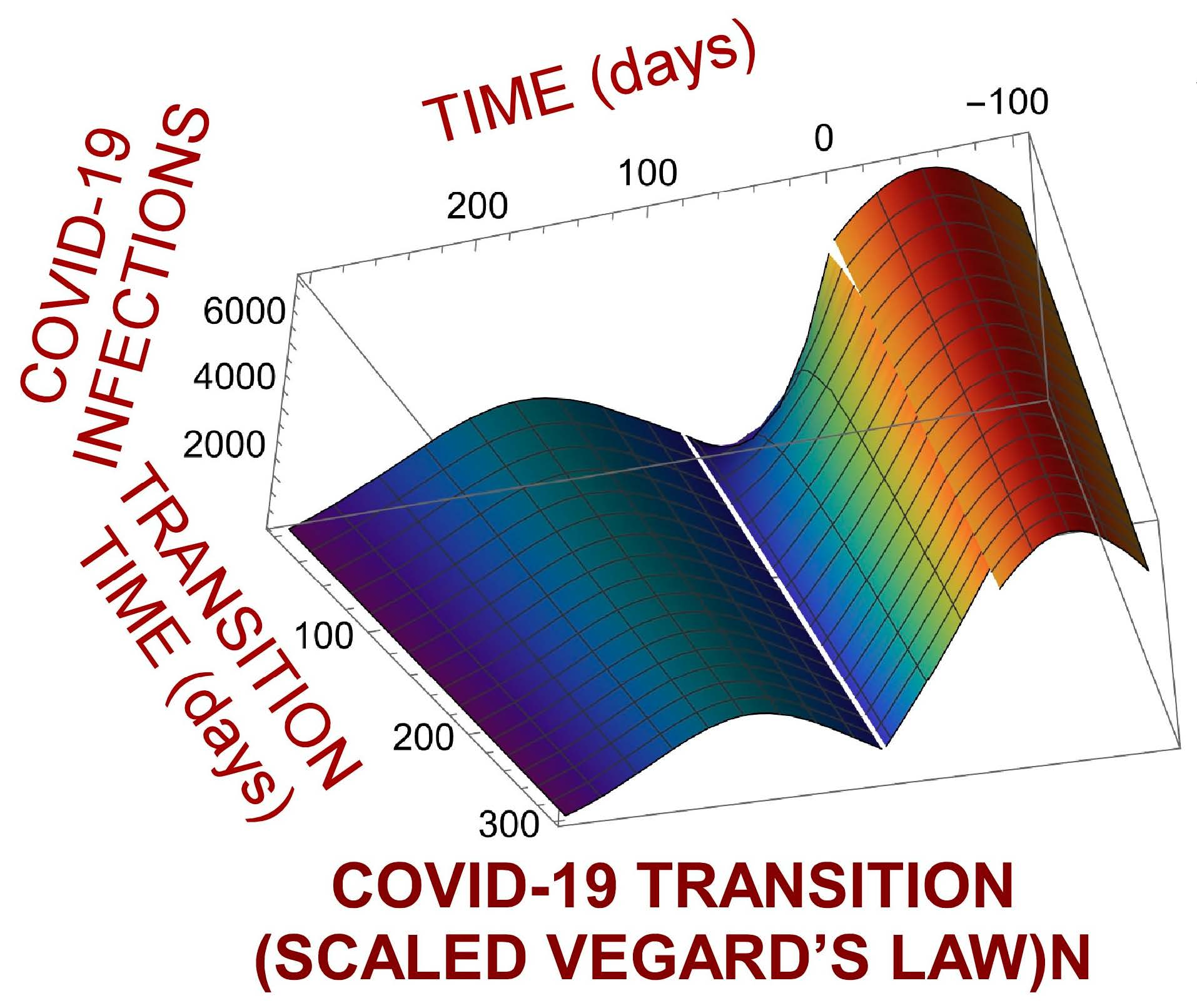
- Vegard, L. Die Konstitution der Mischkristalle und die Raumfüllung der Atome. Z. Für Phys. 1921, 5, 17–26. [Google Scholar] [CrossRef]
- Available online: https://hartfordhealthcaremedicalgroup.org/about-us/news-center/news-detail?articleId=36336&publicid=395 (accessed on 25 October 2023).
- Hu, C. Lucky-electron model of channel hot electron emission. In Proceedings of the 1979 International Electron Devices Meeting, Washington, DC, USA, 3–5 December 1979; pp. 22–25. [Google Scholar] [CrossRef]


| Parameter | Unit | Meaning | Comment |
|---|---|---|---|
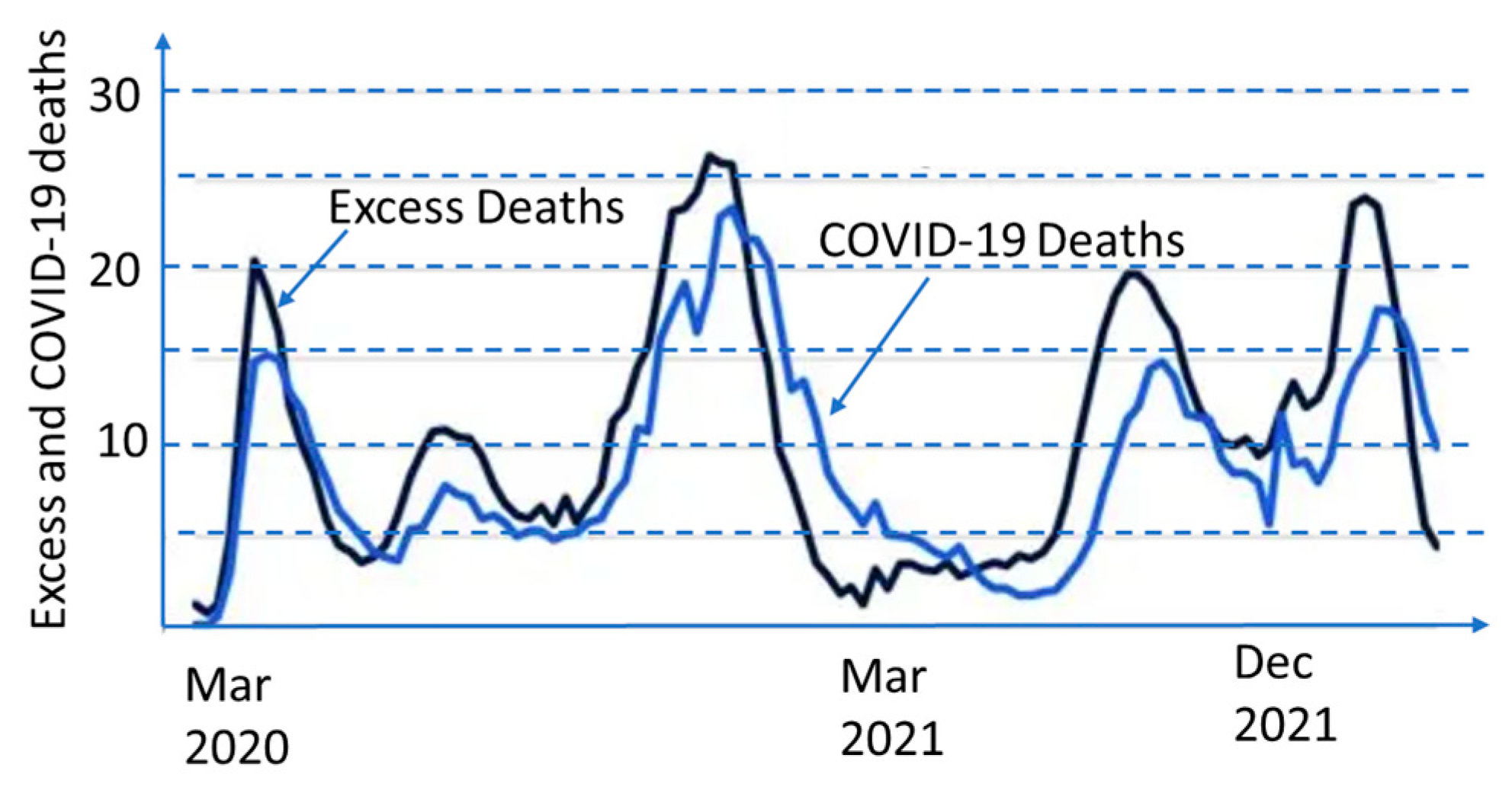
| k | - | The index corresponding to monitoring different pandemic events | k = 1 number of infections, k = 2 number of hospital admissions, k = 3 number of deaths, k = 4 excess mortality numbers |
| w | - | The index corresponding to different mitigation events during pandemic wave | |
| l | - | The index corresponding to different pandemic waves | |
| Nk | The number of people infected from the pandemic start | ||
| Nt | - | Total number of people who could be infected in a local pool | . |
| Nok | Number of infected people at the pandemic start | Typical values 1 to 20 | |
| fok | - | Initial infection ratio | |
| τoκ | day | Initial growth time constant | Typical values from 2 to 5 days |
| τk | day | Time-dependent growth time constant | τk = τok + akτ |
| αk | - | Curve flattening parameter | αk is extracted from pandemic peak time, tm |
| αωk | - | Mitigation event flattening parameter | |
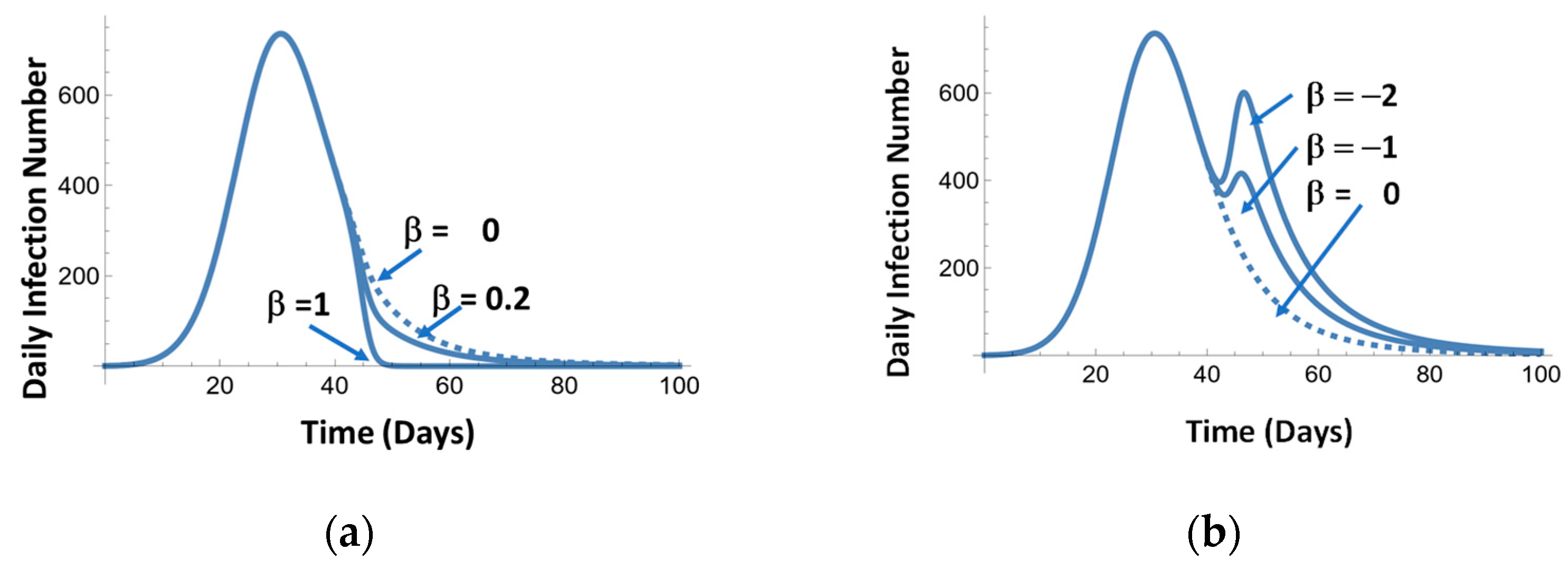
| βkw | - | Mitigation parameters for w = 1, 2, …n mitigation events | Negative β corresponds to lifting restrictions. Typical values −3 to 1 |
| twk | day | Times of mitigation events | Typically, larger than the pandemic peak time |
| τwk | day | Time constants of mitigation events | |
| tm | day | Time of the pandemic peak | |
| Fwk | - | Scaled Fermi–Dirac (FDS) distribution function | |
| q | C | Electronic charge | 1.602 × 10⁻¹⁹ C |
| T | K | Temperature | Degrees Kelvin |
| kB | J/K | Boltzmann constant | 1.38 × 10⁻²³ J/K |
| EF | eV | Fermi level |
Disclaimer/Publisher’s Note: The statements, opinions and data contained in all publications are solely those of the individual author(s) and contributor(s) and not of MDPI and/or the editor(s). MDPI and/or the editor(s) disclaim responsibility for any injury to people or property resulting from any ideas, methods, instructions or products referred to in the content. |
© 2024 by the author. Licensee MDPI, Basel, Switzerland. This article is an open access article distributed under the terms and conditions of the Creative Commons Attribution (CC BY) license (https://creativecommons.org/licenses/by/4.0/).
Share and Cite
Shur, M. Pandemic Equation and COVID-19 Evolution. Encyclopedia 2024, 4, 682-694. https://doi.org/10.3390/encyclopedia4020042
Shur M. Pandemic Equation and COVID-19 Evolution. Encyclopedia. 2024; 4(2):682-694. https://doi.org/10.3390/encyclopedia4020042
Chicago/Turabian StyleShur, Michael. 2024. "Pandemic Equation and COVID-19 Evolution" Encyclopedia 4, no. 2: 682-694. https://doi.org/10.3390/encyclopedia4020042
APA StyleShur, M. (2024). Pandemic Equation and COVID-19 Evolution. Encyclopedia, 4(2), 682-694. https://doi.org/10.3390/encyclopedia4020042