Auto-Correlation Functions of Chaotic Binary Sequences Obtained by Alternating Two Binary Functions

Abstract

This paper discusses the auto-correlation functions of chaotic binary sequences obtained by a one-dimensional chaotic map and two binary functions. The two binary functions are alternately used to obtain a binary sequence from a chaotic real-valued sequence. We consider two similar methods and give the theoretical auto-correlation functions of the new binary sequences, which are expressed by the auto-/cross-correlation functions of the two chaotic binary sequences generated by a single binary function. Furthermore, some numerical experiments are performed to confirm the validity of the theoretical auto-correlation functions.

1. Introduction

One-dimensional (1-D) nonlinear maps can generate chaotic real-valued sequences [1,2] and they can be used as random numbers due to their simplicity, despite their complex behavior [3,4,5,6]. Chaotic real-valued sequences can be transformed into discrete-valued (e.g., binary) sequences using discrete-valued functions, and they have been used in some applications (e.g., CDMA communications as spreading codes) [7]. In 1988, chaotic binary sequences based on a 1-D chaotic map (tent map) were proposed and proven to be independent and identically distributed (i.i.d.) [8]. In 1997, the statistical properties of chaotic binary sequences based on 1-D chaotic maps were deeply discussed and a sufficient condition to generate i.i.d. binary sequences was given for a class of chaotic maps and binary functions [9].

As described above, ideal random numbers are often assumed to be i.i.d. since the most prominent application of chaos-based random numbers is in the area of security, such as cryptography [3,4,5,6]. On the other hand, correlated chaotic sequences have also been discussed, and they are useful in some applications other than cryptography. The auto-correlation functions of chaotic real-valued sequences generated by the skew tent map were theoretically derived in [10], where the auto-correlation functions were exponentially decreasing. Chaotic discrete-valued sequences with exponential auto-correlation functions were discussed in [11,12,13], and some of them can be applied to CDMA communications as spreading codes. In Monte Carlo integration, the convergence rate can be drastically improved by using chaotic sequences with proper auto-correlations, which is called super-efficient chaotic Monte-Carlo simulation [14]. Thus, in applications of chaos-based random numbers, the controllability of the statistical properties is quite important. It should be noted that the desired (or optimal) statistical properties of the random numbers are different depending on the application.

Still, there have been many studies on chaos-based random number generation in both theoretical and experimental contexts (e.g., [15,16,17]). In order to adapt chaos-based random numbers for many applications, we have been attempting to realize chaotic binary (or discrete-valued) sequences with various auto-correlation properties [18]. To generate a chaotic binary sequence, a chaotic map and a binary function are normally used. Of course, there are many combinations of a chaotic map and a binary (or discrete-valued) function, which implies that various statistical properties can be realized. In this paper, however, we propose a different approach to generating chaotic binary sequences using 1-D chaotic maps. We use one chaotic map and two binary functions to generate a chaotic binary sequence, where the two binary functions are alternately used. The theoretical average and auto-correlation function of the new chaotic binary sequence are given, which is followed by numerical experiments using some chaotic maps and binary functions.

The rest of this paper is organized as follows. In Section 2, a brief review of conventional chaotic binary sequences based on 1-D chaotic map is given, where the theoretical average and auto-correlation function are defined. In Section 3, we propose two methods to generate chaotic binary sequences, where a chaotic map and two binary functions are used to generate a chaotic binary sequence. The two binary functions are alternately used. We derive the theoretical auto-correlation functions of the chaotic binary sequences generated by the proposed methods. Numerical results obtained using some chaotic maps and binary functions are shown in Section 4. Finally, Section 5 concludes this paper.

2. Chaotic Binary Sequences Based on a One-Dimensional Map and a Binary Function

A one-dimensional nonlinear difference equation defined by

$$x_{n+1}=\tau \left(x_n\right),x_n\in I=[0,1],n=0,1,2,\cdots$$

(1)

can generate a chaotic real-valued sequence ${\left\{x_n\right\}}_{n=0}^{\infty }$ for a chaotic map $\tau \left(x\right)$ [1,2]. Moreover, we can obtain a binary sequence ${\left\{B\left(x_n\right)\right\}}_{n=0}^{\infty }$ using a binary function $B\left(x\right)(\in \{0,1\left\}\right)$ from a real-valued sequence ${\left\{x_n\right\}}_{n=0}^{\infty }$. Then, the theoretical auto-correlation function of the binary sequence ${\left\{B\left(x_n\right)\right\}}_{n=0}^{\infty }$ is defined by

$$A(\ell ;B)={\int }_I(B\left(x\right)-E\left[B\right])(B\left({\tau }^{\ell }\left(x\right)\right)-E\left[B\right])f^{*}\left(x\right)dx,$$

(2)

under the assumption that $\tau \left(x\right)$ has an invariant density function $f^{*}\left(x\right)$, where ${\tau }^{\ell }\left(x\right)$ is the ℓ-th iterate of the map $\tau$ starting from an initial value $x=x_0$, and $E\left[B\right]$ denotes the average of the binary sequence ${\left\{B\left(x_n\right)\right\}}_{n=0}^{\infty }$ defined by

$$E\left[B\right]={\int }_{I}B\left(x\right)f^{*}\left(x\right)dx.$$

(3)

We also define the normalized auto-correlation function by

$$\tilde{A}(\ell ;B)=\frac{A(\ell ;B)}{A(0;B)},$$

(4)

where $A(0;B)$ is the variance of ${\left\{B\left(x_n\right)\right\}}_{n=0}^{\infty }$. On the other hand, the auto-correlation function of ${\left\{B\left(x_n\right)\right\}}_{n=0}^{\infty }$ in time-average form is defined by

$${\widehat{A}}_N(\ell ;B\left(x_n\right))=\frac{1}{N}\sum _{n=0}^{N-1}(B\left(x_n\right)-E\left[B\right])(B\left(x_{n+\ell }\right)-E\left[B\right]),$$

(5)

which can be used in numerical calculations of auto-correlation functions. According to the Birkhoff individual ergodic theorem [1,2], we have

$${\displaystyle \underset{N\to \infty }{lim}{\widehat{A}}_N(\ell ;B\left(x_n\right))=A(\ell ;B)\mathrm{for} \mathrm{almost} \mathrm{all} x_0.}$$

(6)

Note that the time average of ${\left\{B\left(x_n\right)\right\}}_{n=0}^{\infty }$ is defined by

$${\widehat{E}}_N\left[B\left(x_n\right)\right]=\frac{1}{N}\sum _{n=0}^{N-1}B\left(x_n\right),$$

(7)

and we also have

$$\underset{N\to \infty }{lim}{\widehat{E}}_N\left[B\left(x_n\right)\right]=E\left[B\right]\mathrm{for} \mathrm{almost} \mathrm{all} x_0.$$

(8)

Next, for two chaotic binary sequences ${\left\{B_1\left(x_n\right)\right\}}_{n=0}^{\infty }$ and ${\left\{B_2\left(x_n\right)\right\}}_{n=0}^{\infty }$ generated from a common real-valued sequence ${\left\{x_n\right\}}_{n=0}^{\infty }$, their cross-correlation function is defined by

$$C(\ell ;B_1,B_2)={\int }_I(B_1\left(x\right)-E\left[B_1\right])(B_2\left({\tau }^{\ell }\left(x\right)\right)-E\left[B_2\right])f^{*}\left(x\right)dx.$$

(9)

Note that $C(\ell ;B_1,B_2)=B(\ell ;B_2,B_1)$ does not always hold. The normalized cross-correlation function is defined by

$$\tilde{C}(\ell ;B_1,B_2)=\frac{C(\ell ;B_1,B_2)}{\sqrt{A(0;B_1)}\sqrt{A(0;B_2)}}.$$

(10)

The cross-correlation function between ${\left\{B_1\left(x_n\right)\right\}}_{n=0}^{\infty }$ and ${\left\{B_2\left(x_n\right)\right\}}_{n=0}^{\infty }$ in time-average form is defined by

$${\widehat{C}}_N(\ell ;B_1\left(x_n\right),B_2\left(x_n\right))=\frac{1}{N}\sum _{n=0}^{N-1}(B_1\left(x_n\right)-E\left[B_1\right])(B_2\left(x_{n+\ell }\right)-E\left[B_2\right]).$$

(11)

Similar to (6), we have

$${\displaystyle \underset{N\to \infty }{lim}{\widehat{C}}_N(\ell ;B_1\left(x_n\right),B_2\left(x_n\right))=C(\ell ;B_1,B_2)\mathrm{for} \mathrm{almost} \mathrm{all} x_0.}$$

(12)

3. Chaotic Binary Sequences Obtained by Alternating Two Binary Functions

We use two binary functions $B_1\left(x\right)$ and $B_2\left(x\right)$ to generate a new binary sequence from a chaotic real-valued sequence ${\left\{x_n\right\}}_{n=0}^{\infty }$. We propose the following two methods and discuss the auto-correlation functions of the generated binary sequences.

3.1. Method 1

Using $B_1\left(x\right)$ and $B_2\left(x\right)$ alternately, we generate a new binary sequence ${\left\{D_n^{\left(1\right)}\right\}}_{n=0}^{\infty }$ as

$$B_1\left(x_0\right),B_2\left(x_1\right),B_1\left(x_2\right),B_2\left(x_3\right),\cdots ,$$

(13)

that is,

$$D_n^{\left(1\right)}=\left\{\begin{array}{cc}{B}_1\left(x_n\right)\hfill & (n=0,2,4,\cdots ),\hfill \\ B_2\left(x_n\right)\hfill & (n=1,3,5,\cdots ).\hfill \end{array}\right.$$

(14)

Here, we assume $E\left[B_1\right]=E\left[B_2\right]$, which gives

$$E\left[D_n^{\left(1\right)}\right]=E\left[B_1\right]=E\left[B_2\right].$$

(15)

Next, consider the auto-correlation function of the binary sequence ${\left\{D_n^{\left(1\right)}\right\}}_{n=0}^{\infty }$. First, the auto-correlation function in time-average form is expressed by

$$\begin{array}{cc}\hfill & {\widehat{A}}_N(\ell ;D_n^{\left(1\right)})=\hfill \\ \hfill & \left\{\begin{array}{c}\frac{1}{N}(B_1\left(x_0\right)B_1\left(x_{\ell }\right)+B_2\left(x_1\right)B_2\left(x_{1+\ell }\right)+B_1\left(x_2\right)B_1\left(x_{2+\ell }\right)+B_2\left(x_3\right)B_2\left(x_{3+\ell }\right)+\cdots )\hfill \\ (\ell =0,2,4,\cdots ),\hfill \\ \frac{1}{N}(B_1\left(x_0\right)B_2\left(x_{\ell }\right)+B_2\left(x_1\right)B_1\left(x_{1+\ell }\right)+B_1\left(x_2\right)B_2\left(x_{2+\ell }\right)+B_2\left(x_3\right)B_1\left(x_{3+\ell }\right)+\cdots )\hfill \\ (\ell =1,3,5,\cdots ).\hfill \end{array}\right.\hfill \end{array}$$

(16)

Thus, the theoretical auto-correlation function of ${\left\{D_n^{\left(1\right)}\right\}}_{n=0}^{\infty }$ is given by

$$A(\ell ;D_n^{\left(1\right)})=\left\{\begin{array}{cc}\frac{1}{2}(A(\ell ;B_1)+A(\ell ;B_2))\hfill & (\ell =0,2,4,\cdots ),\hfill \\ \frac{1}{2}(C(\ell ;B_1,B_2)+C(\ell ;B_2,B_1))\hfill & (\ell =1,3,5,\cdots ).\hfill \end{array}\right.$$

(17)

Note that $A(\ell ;D_n^{\left(1\right)})$ is invariant under exchanging $B_1\left(x\right)$ and $B_2\left(x\right)$.

3.2. Method 2

Similar to Method 1, we generate a new binary sequence ${\left\{D_n^{\left(2\right)}\right\}}_{n=0}^{\infty }$ using $B_1\left(x\right)$ and $B_2\left(x\right)$ alternately as

$$B_1\left(x_0\right),B_2\left(x_0\right),B_1\left(x_1\right),B_2\left(x_1\right),\cdots .$$

(18)

That is, for each real value $x_n$, two binary values $B_1\left(x_n\right)$, $B_2\left(x_n\right)$ are generated and $D_n^{\left(2\right)}$ is expressed by

$$D_n^{\left(2\right)}=\left\{\begin{array}{cc}{B}_1\left(x_{\frac{n}{2}}\right)\hfill & (n=0,2,4,\cdots ),\hfill \\ B_2\left(x_{\frac{n-1}{2}}\right)\hfill & (n=1,3,5,\cdots ).\hfill \end{array}\right.$$

(19)

We also assume $E\left[B_1\right]=E\left[B_2\right]$, which gives

$$E\left[D_n^{\left(2\right)}\right]=E\left[B_1\right]=E\left[B_2\right].$$

(20)

The auto-correlation function of ${\left\{D_n^{\left(2\right)}\right\}}_{n=0}^{\infty }$ in time-average form is expressed by

$$\begin{array}{cc}\hfill & {\widehat{A}}_N(\ell ;D_n^{\left(2\right)})=\hfill \\ \hfill & \left\{\begin{array}{c}\frac{1}{N}(B_1\left(x_0\right)B_1\left(x_{\frac{\ell }{2}}\right)+B_2\left(x_0\right)B_2\left(x_{\frac{\ell }{2}}\right)+B_1\left(x_1\right)B_1\left(x_{1+\frac{\ell }{2}}\right)+B_2\left(x_1\right)B_2\left(x_{1+\frac{\ell }{2}}\right)+\cdots )\hfill \\ (\ell =0,2,4,\cdots ),\hfill \\ \frac{1}{N}(B_1\left(x_0\right)B_2\left(x_{\frac{\ell -1}{2}}\right)+B_2\left(x_0\right)B_1\left(x_{\frac{\ell +1}{2}}\right)+B_1\left(x_1\right)B_2\left(x_{1+\frac{\ell -1}{2}}\right)+B_2\left(x_1\right)B_1\left(x_{1+\frac{\ell +1}{2}}\right)+\cdots )\hfill \\ (\ell =1,3,5,\cdots ).\hfill \end{array}\right.\hfill \end{array}$$

(21)

Thus, the theoretical auto-correlation function of ${\left\{D_n^{\left(2\right)}\right\}}_{n=0}^{\infty }$ is given by

$$A(\ell ;D_n^{\left(2\right)})=\left\{\begin{array}{cc}\frac{1}{2}(A(\frac{\ell }{2};B_1)+A(\frac{\ell }{2};B_2))\hfill & (\ell =0,2,4,\cdots ),\hfill \\ \frac{1}{2}(C(\frac{\ell -1}{2};B_1,B_2)+C(\frac{\ell +1}{2};B_2,B_1))\hfill & (\ell =1,3,5,\cdots ).\hfill \end{array}\right.$$

(22)

Note that $A(\ell ;D_n^{\left(2\right)})$ is not invariant under the exchange of $B_1\left(x\right)$ and $B_2\left(x\right)$.

4. Numerical Experiments

We perform numerical experiments on Method 1 and Method 2 using three chaotic maps $(I=[0,1],f^{*}\left(x\right)=1)$ and some binary functions. Note that the chaotic maps and the binary functions are chosen as examples to obtain some interesting (or unique) auto-/cross-correlation functions.

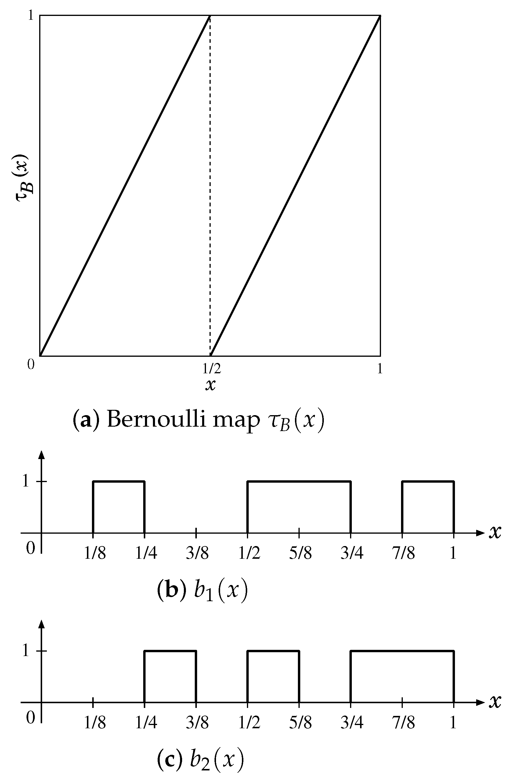
4.1. Bernoulli Map and Binary Functions

The Bernoulli map with $I=[0,1]$ is defined by [1,2]

$${\tau }_B\left(x\right)=\left\{\begin{array}{cc}2x\hfill & (0\le x<\frac{1}{2}),\hfill \\ 2x-1\hfill & (\frac{1}{2}\le x\le 1).\hfill \end{array}\right.$$

(23)

For this map, we use the following two binary functions:

$$\begin{array}{cc}\hfill b_1\left(x\right)& ={\Theta }_{\frac{1}{8}}\left(x\right)-{\Theta }_{\frac{1}{4}}\left(x\right)+{\Theta }_{\frac{1}{2}}\left(x\right)-{\Theta }_{\frac{3}{4}}\left(x\right)+{\Theta }_{\frac{7}{8}}\left(x\right),\hfill \end{array}$$

(24)

$$\begin{array}{cc}\hfill b_2\left(x\right)& ={\Theta }_{\frac{1}{4}}\left(x\right)-{\Theta }_{\frac{3}{8}}\left(x\right)+{\Theta }_{\frac{1}{2}}\left(x\right)-{\Theta }_{\frac{5}{8}}\left(x\right)+{\Theta }_{\frac{3}{4}}\left(x\right),\hfill \end{array}$$

(25)

where ${\Theta }_t\left(x\right)$ is a threshold function with a threshold t defined by

$${\Theta }_t\left(x\right)=\left\{\begin{array}{cc}0& (x<t),\hfill \\ 1& (x\ge t).\hfill \end{array}\right.$$

(26)

The Bernoulli map ${\tau }_B\left(x\right)$ and the binary functions $b_1\left(x\right)$, $b_2\left(x\right)$ are illustrated in Figure 1. Since the Bernoulli map has $f^{*}\left(x\right)=1$ (uniform density), we have

$$E\left[b_1\right]=E\left[b_2\right]=\frac{1}{2},$$

(27)

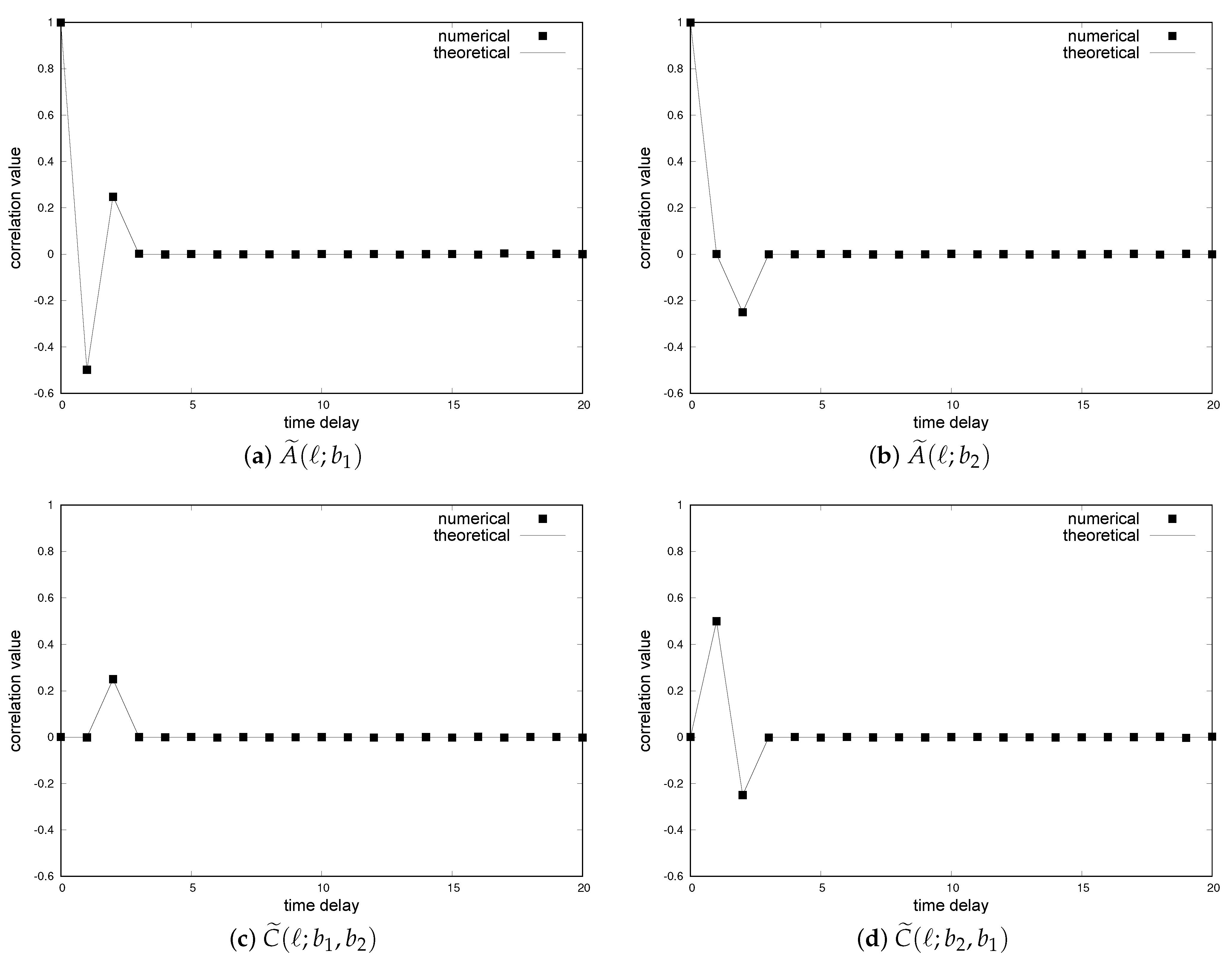
that is, the binary sequences ${\left\{b_1\left({\tau }_B^n\left(x\right)\right)\right\}}_{n=0}^{\infty }$ and ${\left\{b_2\left({\tau }_B^n\left(x\right)\right)\right\}}_{n=0}^{\infty }$ are balanced sequences. The theoretical correlation functions of the binary sequences can be derived by referring to [9,13] (see Appendix A for details). The normalized theoretical auto-/cross-correlation functions of the two binary sequences are summarized in

Table 1. Normalized theoretical auto-/cross-correlation functions of ${\left\{b_1\left({\tau }_B^n\left(x\right)\right)\right\}}_{n=0}^{\infty }$ and ${\left\{b_2\left({\tau }_B^n\left(x\right)\right)\right\}}_{n=0}^{\infty }$.

	$\mathit{\ell }=0$	$\mathit{\ell }=1$	$\mathit{\ell }=2$	$\mathit{\ell }\ge 3$
$\tilde{A}(\ell ;b_1)$	1	$-\frac{1}{2}$	$\frac{1}{4}$	0
$\tilde{A}(\ell ;b_2)$	1	0	$-\frac{1}{4}$	0
$\tilde{C}(\ell ;b_1,b_2)$	0	0	$\frac{1}{4}$	0
$\tilde{C}(\ell ;b_2,b_1)$	0	$\frac{1}{2}$	$-\frac{1}{4}$	0

and illustrated in Figure 2. In Figure 2, numerical auto-/cross-correlation functions calculated by (5) and (11) with $N={10}^6$ are also shown.

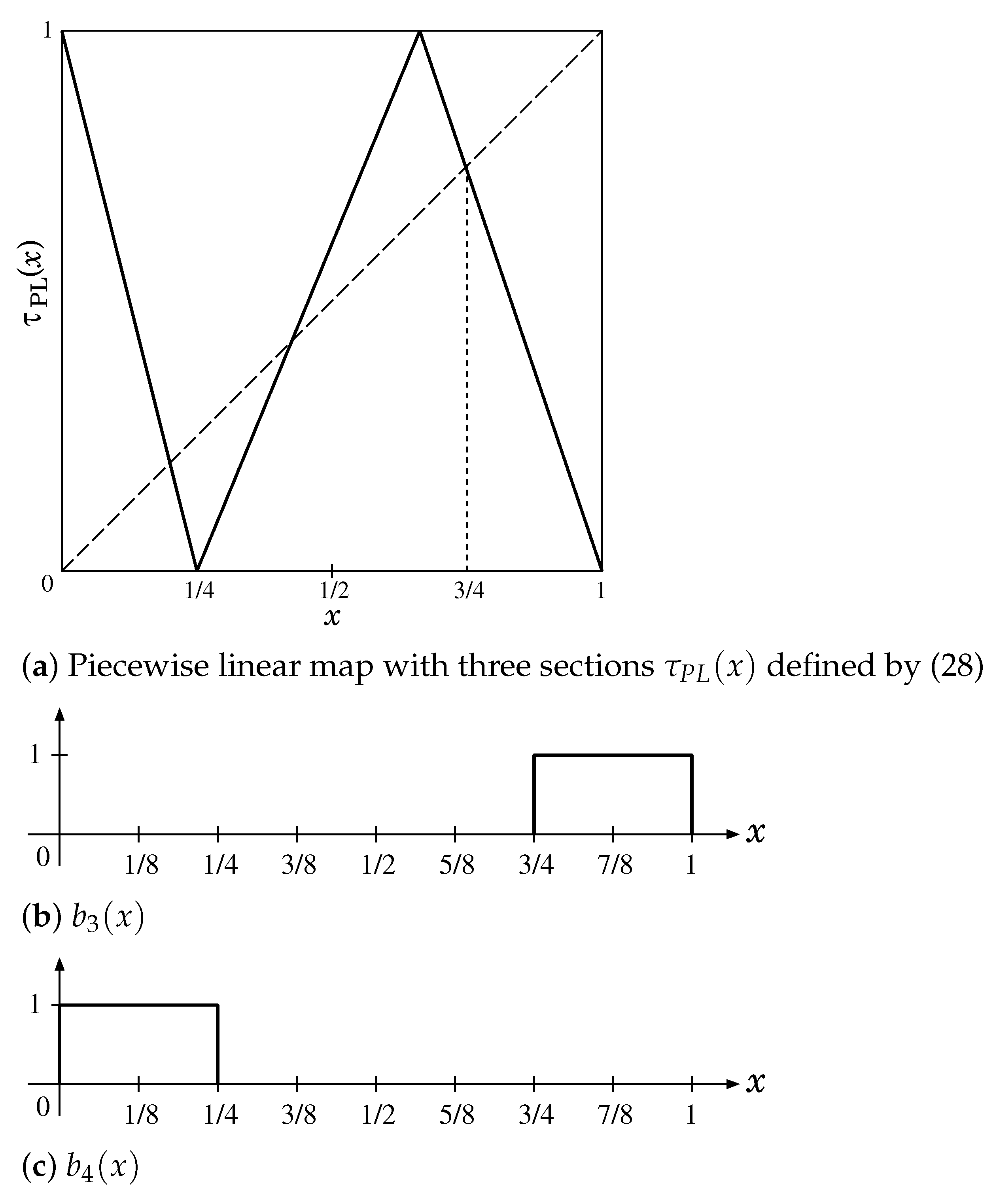
4.2. Piecewise Linear Map with Three Sections and Binary Functions

Define a fully stretching piecewise linear (PL) map with $I=[0,1]$ by [13]

$${\tau }_{PL}\left(x\right)=\left\{\begin{array}{cc}\hfill -4x+1& (0\le x<\frac{1}{4}),\hfill \\ \hfill \frac{12}{5}x-\frac{3}{5}& (\frac{1}{4}\le x<\frac{2}{3}),\hfill \\ \hfill -3x+3& (\frac{2}{3}\le x\le 1).\hfill \end{array}\right.$$

(28)

For this map, we use the following two binary functions:

$$\begin{array}{cc}\hfill b_3\left(x\right)& ={\Theta }_{\frac{3}{4}}\left(x\right),\hfill \end{array}$$

(29)

$$\begin{array}{cc}\hfill b_4\left(x\right)& =1-{\Theta }_{\frac{1}{4}}\left(x\right).\hfill \end{array}$$

(30)

The PL map ${\tau }_{PL}\left(x\right)$ and the binary functions $b_3\left(x\right)$, $b_4\left(x\right)$ are illustrated in Figure 3. Since the PL map ${\tau }_{PL}\left(x\right)$ also has $f^{*}\left(x\right)=1$, we have

$$E\left[b_3\right]=E\left[b_4\right]=\frac{1}{4},$$

(31)

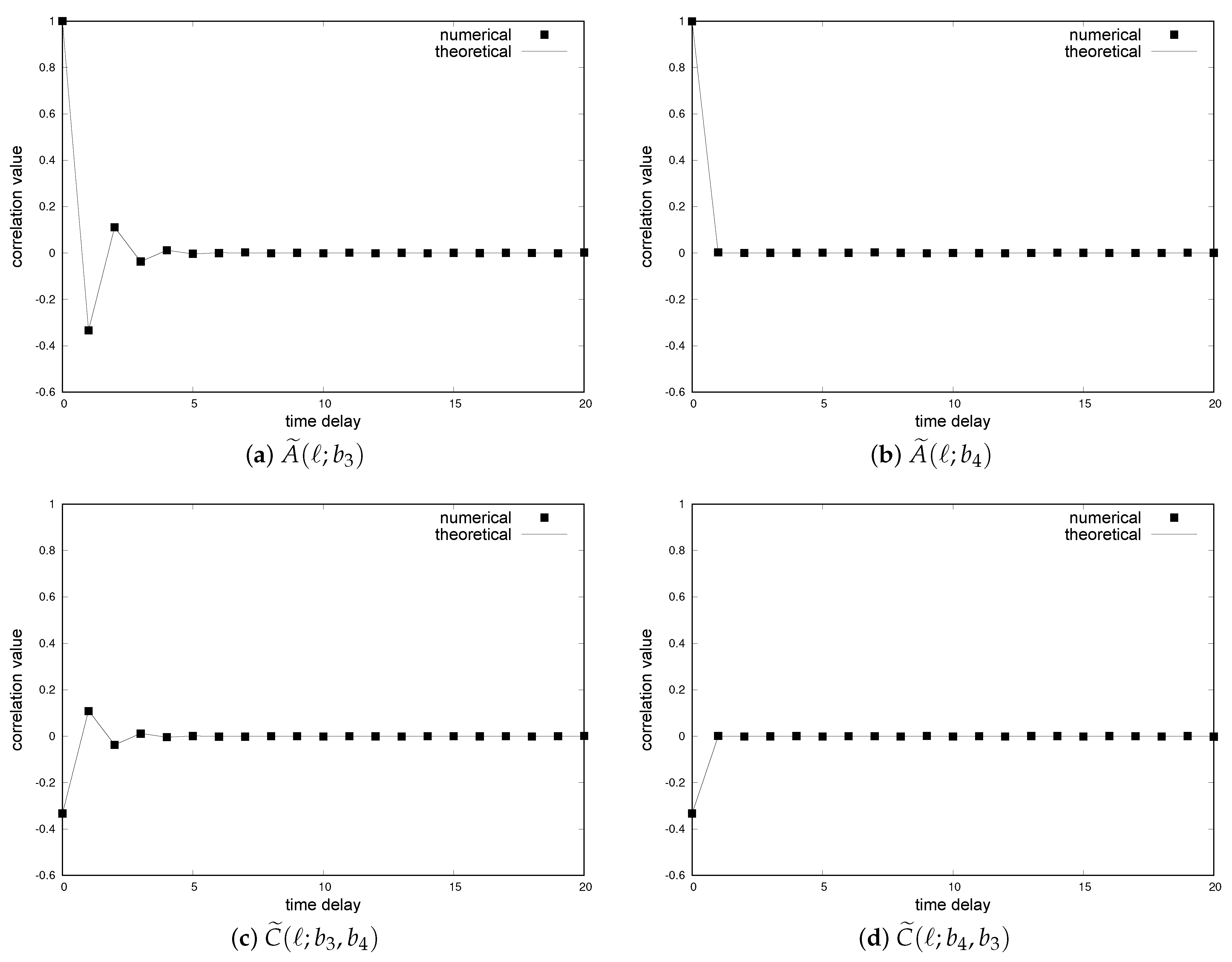
that is, the binary sequences ${\left\{b_3\left({\tau }_{PL}^n\left(x\right)\right)\right\}}_{n=0}^{\infty }$ and ${\left\{b_4\left({\tau }_{PL}^n\left(x\right)\right)\right\}}_{n=0}^{\infty }$ are unbalanced sequences. The theoretical correlation functions of the binary sequences can be derived by referring to [9,13] (see Appendix A for details). The normalized theoretical auto-/cross-correlation functions of the two binary sequences are summarized in

Table 2. Normalized theoretical auto-/cross-correlation functions of ${\left\{b_3\left({\tau }_{PL}^n\left(x\right)\right)\right\}}_{n=0}^{\infty }$ and ${\left\{b_4\left({\tau }_{PL}^n\left(x\right)\right)\right\}}_{n=0}^{\infty }$.

	$\mathit{\ell }=0$	$\mathit{\ell }=1$	$\mathit{\ell }=2$	$\mathit{\ell }\ge 3$
$\tilde{A}(\ell ;b_3)$	${(-3)}^{-\ell }$
$\tilde{A}(\ell ;b_4)$	1	0	0	0
$\tilde{C}(\ell ;b_3,b_4)$	${(-3)}^{-\ell -1}$
$\tilde{C}(\ell ;b_4,b_3)$	$-\frac{1}{3}$	0	0	0

and illustrated in Figure 4. In Figure 4, numerical auto-/cross-correlation functions calculated by (5) and (11) with $N={10}^6$ are also shown.

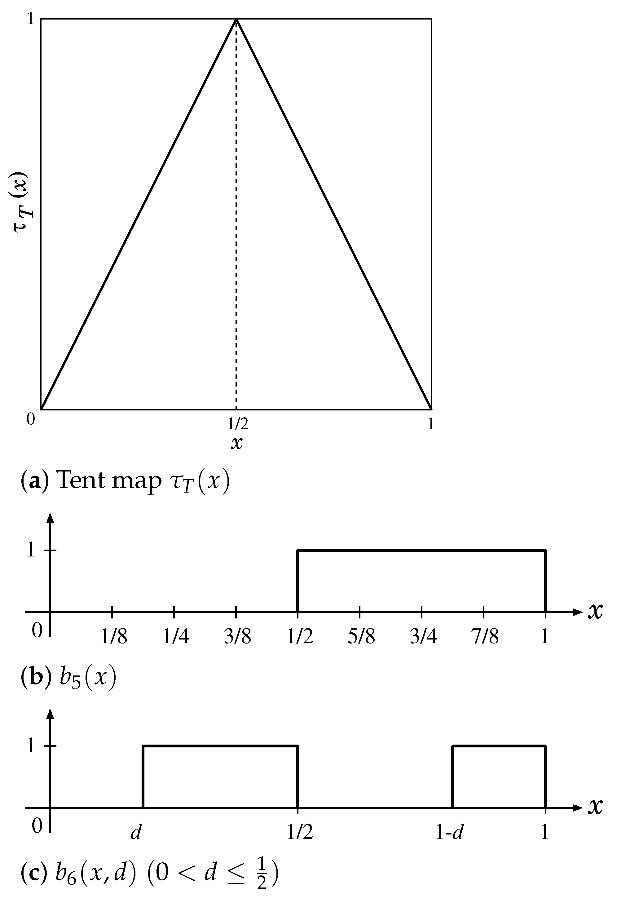
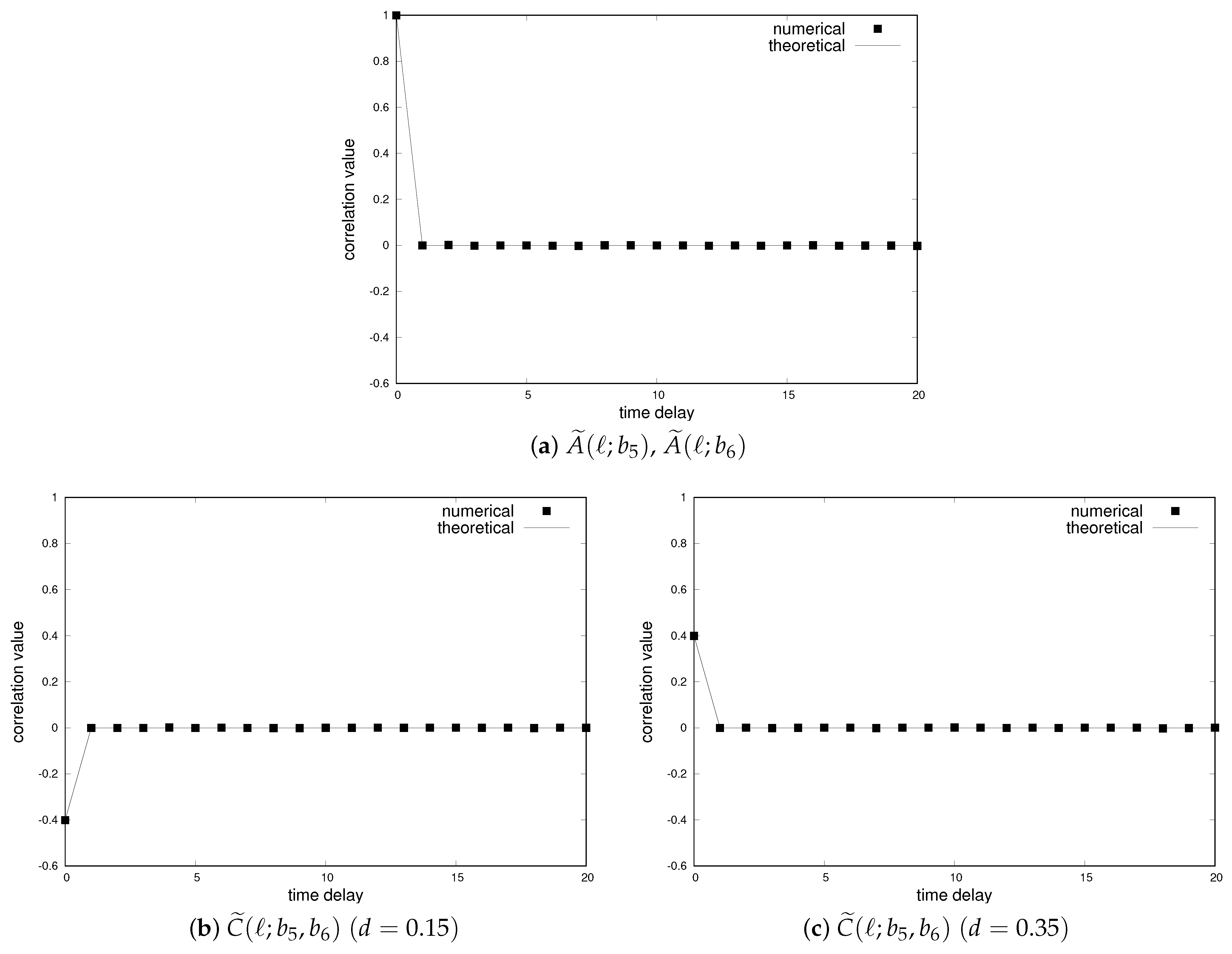
4.3. Tent Map and Binary Functions

Define the tent map with $I=[0,1]$ by [1,2,10]

$${\tau }_T\left(x\right)=\left\{\begin{array}{cc}2x\hfill & (0\le x<\frac{1}{2}),\hfill \\ 2(1-x)\hfill & (\frac{1}{2}\le x\le 1).\hfill \end{array}\right.$$

(32)

For this map, we use the following two binary functions:

$$\begin{array}{cc}\hfill b_5\left(x\right)& ={\Theta }_{\frac{1}{2}}\left(x\right),\hfill \end{array}$$

(33)

$$\begin{array}{cc}\hfill b_6(x,d)& ={\Theta }_d\left(x\right)-{\Theta }_{\frac{1}{2}}\left(x\right)+{\Theta }_{1-d}\left(x\right)(0<d\le \frac{1}{2}).\hfill \end{array}$$

(34)

The tent map ${\tau }_T\left(x\right)$ and the binary functions $b_5\left(x\right)$, $b_6\left(x\right)$ are illustrated in Figure 5. Since the tent map ${\tau }_T\left(x\right)$ also has $f^{*}\left(x\right)=1$, we have

$$E\left[b_5\right]=E\left[b_6\right]=\frac{1}{2},$$

(35)

that is, the binary sequences ${\left\{b_5\left({\tau }_T^n\left(x\right)\right)\right\}}_{n=0}^{\infty }$ and ${\left\{b_6({\tau }_T^n\left(x\right),d)\right\}}_{n=0}^{\infty }$ are balanced sequences. The theoretical correlation functions of the binary sequences can be derived by referring to [9,13] (see Appendix A for details). Actually, ${\left\{b_5\left({\tau }_T^n\left(x\right)\right)\right\}}_{n=0}^{\infty }$ and ${\left\{b_6({\tau }_T^n\left(x\right),d)\right\}}_{n=0}^{\infty }$ are i.i.d. and uncorrelated to each other for $\ell \ge 1$. Note that the cross-correlation function for $\ell =0$, $C(0;b_5,b_6)$, can be controlled by d (parameter of the binary function $b_6(x,d)$). The normalized theoretical auto-/cross-correlation functions of the two binary sequences are summarized in

Table 3. Normalized theoretical auto-/cross-correlation functions of ${\left\{b_5\left({\tau }_T^n\left(x\right)\right)\right\}}_{n=0}^{\infty }$ and ${\left\{b_6({\tau }_T^n\left(x\right),d)\right\}}_{n=0}^{\infty }$.

	$\mathit{\ell }=0$	$\mathit{\ell }\ge 1$
$\tilde{A}(\ell ;b_5)$	1	0
$\tilde{A}(\ell ;b_6)$	1	0
$\tilde{C}(\ell ;b_5,b_6)$	$4d-1$	0

and illustrated in Figure 6. In Figure 6, numerical auto-/cross-correlation functions calculated by (5) and (11) with $N={10}^6$ are also shown.

4.4. Auto-Correlation Functions of New Binary Sequences by Method 1 and Method 2

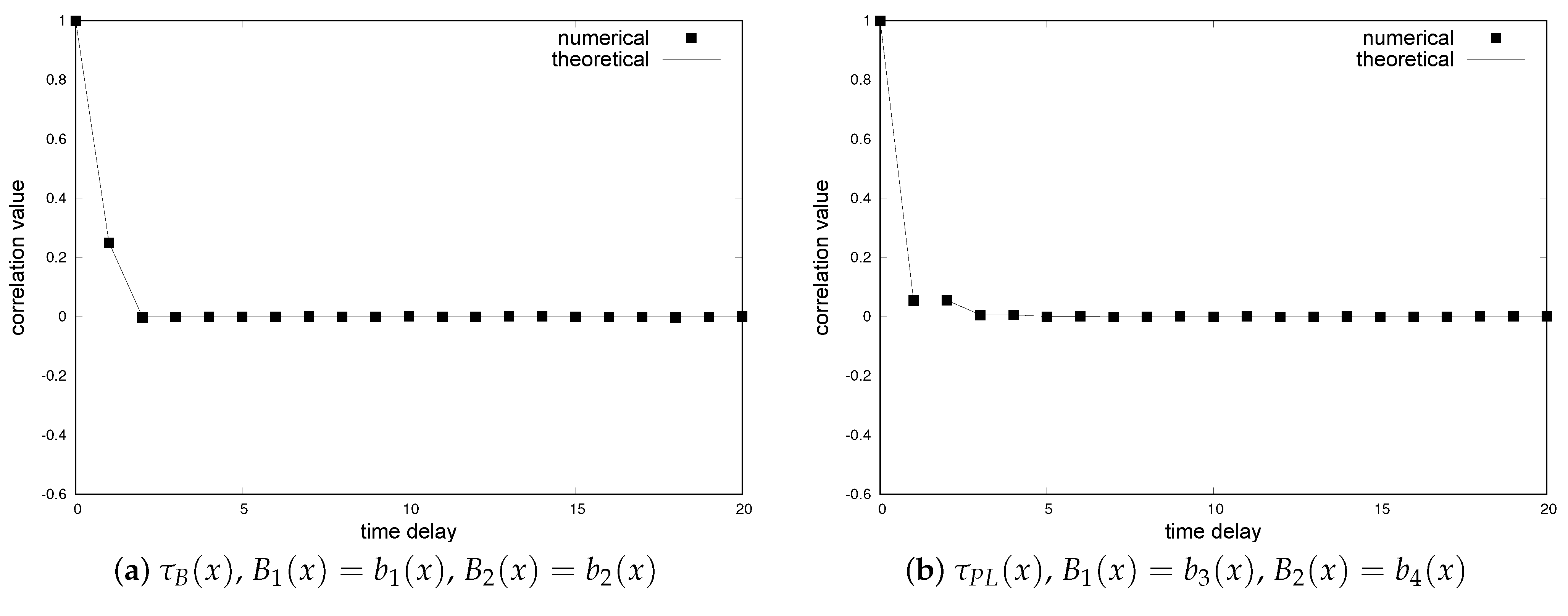
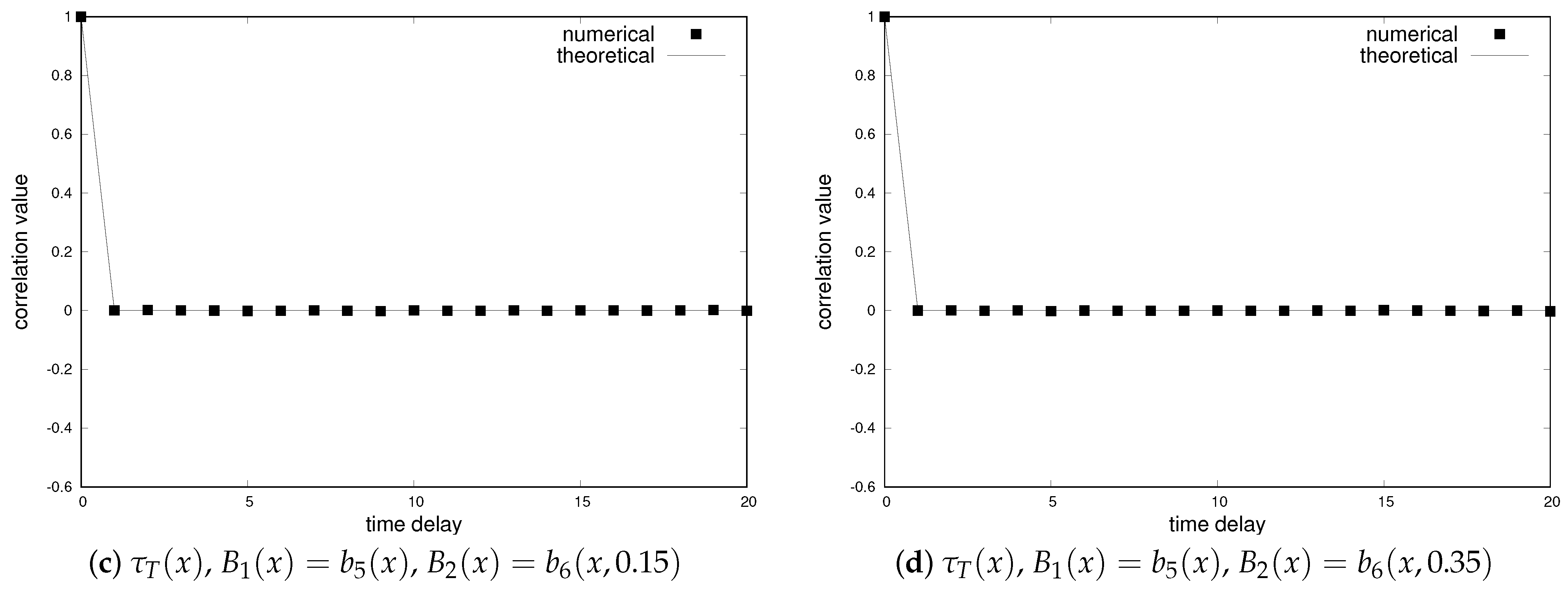
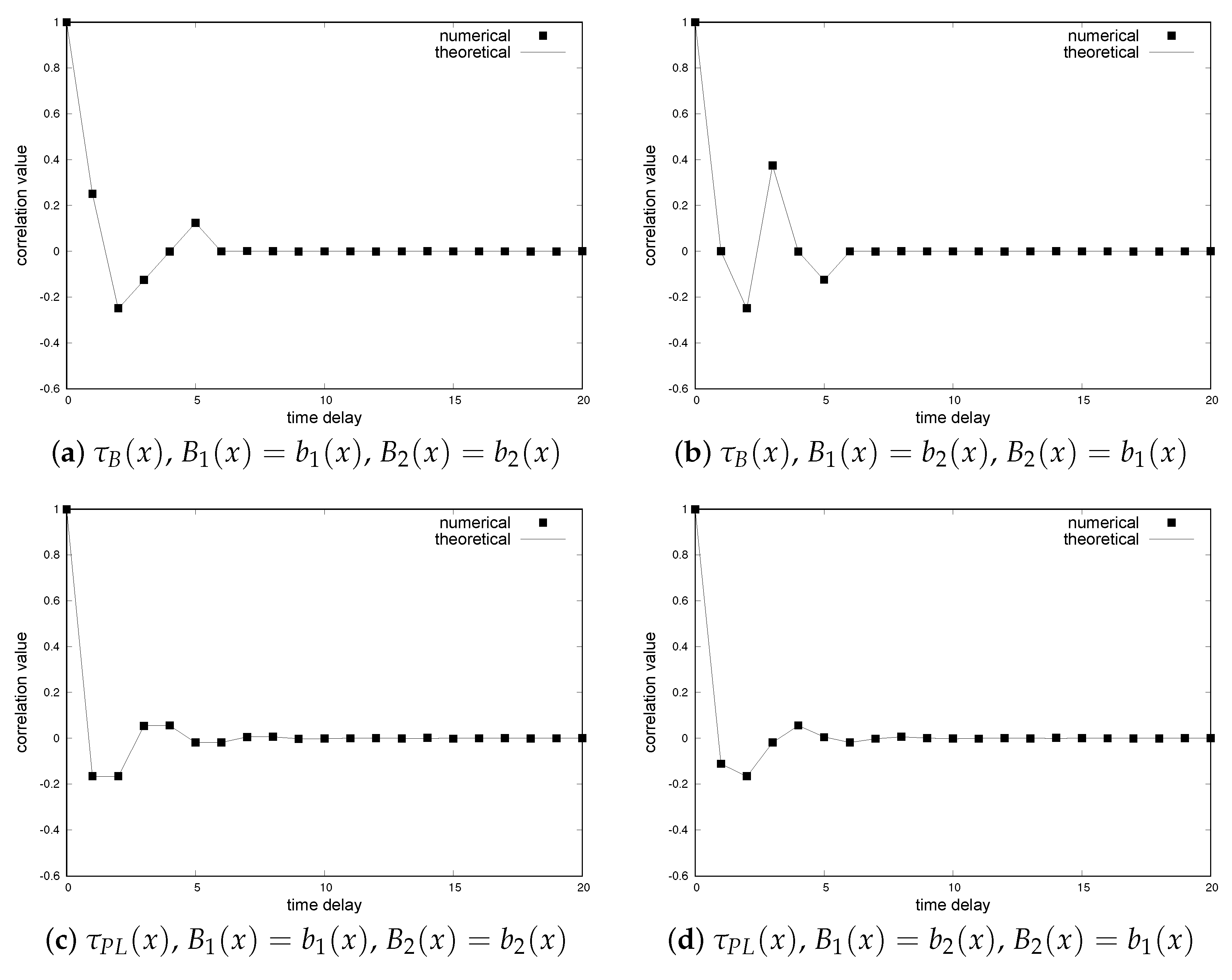
First, Figure 7 shows the normalized auto-correlation functions of new binary sequences ${\left\{D_n^{\left(1\right)}\right\}}_{n=0}^{\infty }$ in Method 1, where the theoretical auto-correlation functions are calculated by (17) and the numerical ones are calculated by (5), where $N={10}^6$. We can find that the auto-correlation functions of ${\left\{D_n^{\left(1\right)}\right\}}_{n=0}^{\infty }$ given in Figure 7a,b are different from those of the original binary sequences, but Figure 7c,d show the uncorrelated property, which is the same as in the original two binary sequences. We also confirm that the theoretical and numerical ones are in good agreement.

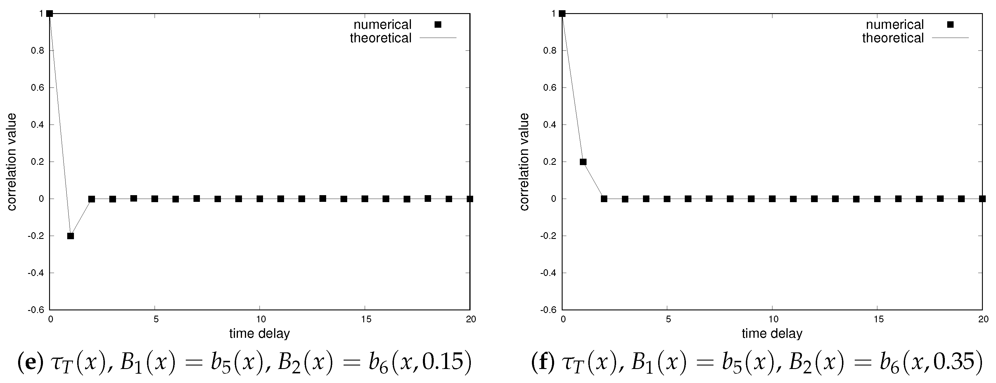
Next, Figure 8 shows the normalized auto-correlation functions of new binary sequences ${\left\{D_n^{\left(2\right)}\right\}}_{n=0}^{\infty }$ in Method 2, where the theoretical auto-correlation functions are calculated by (22) and the numerical ones are calculated by (5), where $N={10}^6$. We can find that the auto-correlation functions of ${\left\{D_n^{\left(2\right)}\right\}}_{n=0}^{\infty }$ are different from those of the original binary sequences, and the theoretical and numerical ones are in good agreement. Moreover, it is confirmed that the auto-correlation functions change if $B_1\left(x\right)$ and $B_2\left(x\right)$ are exchanged. It should be noted that the auto-correlation value at $\ell =1$ in (e) and (f) (Figure 8) can be controlled by the parameter d.

5. Conclusions

The auto-correlation functions of chaotic binary sequences obtained by alternating two binary functions are discussed. Their theoretical auto-correlation function is given and verified by numerical experiments. The proposed methods give more flexibility in designing chaotic sequences with various auto-correlation properties (for example, they can be applied to the method in [18]). The number of binary functions can be extended to three or larger numbers, which will be discussed in future work.

References

- Lasota, A.; Mackey, M.C. Chaos, Fractals, and Noise; Springer: New York, NY, USA, 1994. [Google Scholar]
- Boyarsky, A.; Góra, P. Laws of Chaos; Birkhäuser Boston: Boston, MA, USA, 1997. [Google Scholar]
- Gerosa, A.; Bernardini, R.; Pietri, S. A fully integrated chaotic system for the generation of truly random numbers. IEEE Trans. Circuits Syst. I 2001, 49, 993–1000. [Google Scholar] [CrossRef]
- Stojanovski, T.; Kocarev, L. Chaos-based random number generators—Part I: Analysis. IEEE Trans. Circuits Syst. I 2001, 48, 281–288. [Google Scholar] [CrossRef]
- Cicek, I.; Pusane, A.E.; Dundar, G. A novel design method for discrete time chaos based true random number generators. Integr. VLSI J. 2014, 47, 38–47. [Google Scholar] [CrossRef]
- Li, C.; Feng, B.; Li, S.; Kurths, J.; Chen, G. Dynamic analysis of digital chaotic maps via state-mapping networks. IEEE Trans. Circuits Syst. I 2019, 66, 2322–2335. [Google Scholar] [CrossRef]
- Kennedy, M.P.; Rovatti, R.; Setti, G. (Eds.) Chaotic Electronics in Telecommunications; CRC: Boca Raton, FL, USA, 2000. [Google Scholar]
- Liu, Z.; Tang, J.; Yu, J. An application of chaos: Generating binary pseudo-random sequences. In Proceedings of the 1988 IEEE International Symposium on Circuits and Systems, Espoo, Finland, 7–9 June 1988; pp. 1–3. [Google Scholar]
- Kohda, T.; Tsuneda, A. Statistics of chaotic binary sequences. IEEE Trans. Inf. Theory 1997, 43, 104–112. [Google Scholar] [CrossRef]
- Sakai, H.; Tokumaru, H. Autocorrelations of a certain chaos. IEEE Trans. Acoust. Speech Signal Process 1980, 28, 588–590. [Google Scholar] [CrossRef]
- Rovatti, R.; Mazzini, G. Interference in DS-CDMA systems with exponentially vanishing autocorrelations: Chaos-based spreading is optimal. Electron. Lett. 1998, 34, 1911–1913. [Google Scholar] [CrossRef]
- Mazzini, G.; Rovatti, R.; Setti, G. Interference minimization by autocorrelation shaping in asynchronous DS-CDMA systems: Chaos-based spreading is nearly optimal. Electron. Lett. 1999, 35, 1054–1055. [Google Scholar] [CrossRef]
- Tsuneda, A. Design of binary sequences with tunable exponential autocorrelations and run statistics based on one-dimensional chaotic maps. IEEE Trans. Circuits Syst. I 2005, 52, 454–462. [Google Scholar] [CrossRef]
- Yang, C.A.; Yao, K.; Umeno, K.; Biglieri, E. Using deterministic chaos for superefficient Monte-Carlo simulations. IEEE Circuits Syst. Mag. 2013, 13, 26–35. [Google Scholar] [CrossRef]
- Souza, C.E.C.; Chaves, D.P.B.; Pimentel, C. One-dimensional pseudo-chaotic sequences based on the discrete Arnold’s cat map over Z3m. IEEE Trans. Circuits Syst. II 2021, 68, 491–495. [Google Scholar]
- Paul, P.S.; Sadia, M.; Hossain, M.R.; Muldrey, B.; Hasan, M.S. Cascading CMOS-based chaotic maps for improved performance and its application in efficient RNG design. IEEE Access 2022, 10, 33758–33770. [Google Scholar] [CrossRef]
- Tang, J.; Zhang, Z.; Chen, P.; Huang, Z.; Huang, T. A simple chaotic model with complex chaotic behaviors and its hardware implementation. IEEE Trans. Circuits Syst. I 2023, 70, 3676–3688. [Google Scholar] [CrossRef]
- Tsuneda, A. Various Auto-correlation functions of m-bit random numbers generated from chaotic binary sequences. Entropy 2021, 23, 1295. [Google Scholar] [CrossRef]