System Identification Using Self-Adaptive Filtering Applied to Second-Order Gradient Materials

Abstract

For many engineering applications, it is sufficient to use the concept of simple materials. However, higher gradients of the kinematic variables are taken into account to model materials with internal length scales as well as to describe localization effects using gradient theories in finite plasticity or fluid mechanics. In many approaches, length scale parameters have been introduced that are related to a specific micro structure. An alternative approach is possible, if a thermodynamically consistent framework is used for material modeling, as shown in the present contribution. However, even if sophisticated and thermodynamically consistent material models can be established, there are still not yet standard experiments to determine higher order material constants. In order to contribute to this ongoing discussion, system identification based on the method of self-adaptive filtering is proposed in this paper. To evaluate the effectiveness of this approach, it has been applied to second-order gradient materials considering longitudinal vibrations. Based on thermodynamically consistent models that have been solved numerically, it has been possible to prove that system identification based on self-adaptive filtering can be used effectively for both narrow-band and broadband signals in the field of second-order gradient materials. It has also been found that the differences identified for simple materials and gradient materials allow for condition monitoring and detection of gradient effects in the material behavior.

1. Introduction

For many engineering applications, it is sufficient to use the concept of simple materials [1] that includes only first gradients of the kinematical variables. However, in various fields, modern continuum mechanics is also driven by applications that include higher gradients [2]. This is particularly true for materials with a micro-structure, functionally graded materials, and metamaterials [3,4,5,6,7,8]. Furthermore, finite gradient plasticity [9,10] and theories for gradient fluids [11,12,13] became blossoming fields of research in the last few decades. Because of the broad range of research in this field, the list of references is restricted to recent publications. For this reason, the latter is far from being complete. The author therefore apologizes to any colleague not mentioned in spite of their important contributions to academic and/or applied research on gradient materials.

The same holds for theories that have been developed for vibrational problems and wave propagation. However, common for many of these theories is the assumption of an underlying micro-structure characterized by a micro-displacement, as proposed for linear elastic continua by Mindlin [14]. Nowadays, such a continuum theory has been applied to model anti-plane surface waves in an elastic half-space [15]. Also, one-dimensional gradient elasticity models have been derived from a discrete microstructure using continualization methods [16]. The static and dynamic responses of these models have been analyzed in [17].

A comprehensive overview of formulations of gradient elasticity is given in [18]. In this reference, so-called dynamically consistent models based on at least two length scale parameters are discussed. In particular, it is shown that one scalar length scale parameter in combination with strain gradients is relevant for statics, while a second one can, in combination with acceleration gradients, be added for use in dynamics. A purely strain gradient approach that has been applied for longitudinal vibration analysis of microbars using three different length scale parameters has been proposed in [19].

Analytical solutions for thermal vibrations of strain gradient beams considering one internal length scale parameter for the strain gradient have been reported in [20]. Furthermore, optimal vibration control of gradient materials based on a dynamically consistent approach with two length scale parameters has been studied in [21].

However, even if sophisticated and thermodynamically consistent material models can be established, there are still no standard experiments to determine length scale parameter or higher order material constants [22]. To solve this problem, it is possible to apply atomistic simulation approaches [23]. An alternative approach is the application of system identification approaches that have been established in the theory of mechanical vibrations. For simple materials, system identification based on resonance measurements has been proposed [24,25]. Recently, an inverse identification approach based on results of impulse response measurements was proposed in [26].

It is obvious that especially for linear time-invariant (LTI) systems that are composed of structures described by material models considering higher gradients of the kinematical variables, the question of system identification needs further discussion. Contributing to this discussion is the motivation for the present paper. In order to avoid restrictions, the presented approach is embedded in a thermodynamically consistent continuum theory of second-order gradient materials [2] without further specification of internal micro-structures or length scales that are linked to specific strain or acceleration gradients. This allows for a consistent formulation of the governing equations of LTI systems using longitudinal vibrations in finite one-dimensional wave guides as an illustrative example. Such systems can be identified by adaptive filtering considering self-adaptive identification schemas based on the least mean square (LMS) algorithm [27]. To the best knowledge of the author, this paper reports on the application of adaptive filtering for system identification considering second-order gradient materials for the first time.

The introduction of the well-established concept of adaptive filtering to gradient elasticity enables the development of novel and comparable identification approaches based on input–output relations, such as impulse response functions (IRF) or frequency response functions (FRF), that are independent of knowledge about an underlying micro-structure. This is the key motivation for the investigation presented in this paper. Thus, the combination of gradient elasticity and adaptive filtering can been seen as a new contribution to the academic discussion.

However, it is also possible to motivate practical applications, one of which can be connected with computational material design. If it is possible to derive input–output relations for LTI systems with gradient material properties (that do not yet exist) using numerical models, it is possible to include the identified input–output relations into conventional simulation models before manufacturing real world materials. This enables performance evaluations on the material, compound, structural, and/or system level, before dealing with time-consuming and cost-intensive manufacturing problems. Another application can be considered if structural health monitoring is taken into account. In a situation in which the measured real-world IRF (or FRF) of the system that is monitored differs from the nominal one, the change could be used as an indicator for the development of an internal microstructure. If, furthermore, such a change is compared to the change in the input–output relation of an associated virtual twin that includes gradient material effects, it could also be possible to localize the position of the structural change. This could be carried out using a model update procedure based on minimizing the difference between the measured and the simulated input–output relations.

This paper is structured as follows: All aspects of material modeling, necessary to describe and investigate longitudinal vibrations of finite one-dimensional wave guides considering both simple materials and second-order gradient materials, are described in Section 2. The associated numerical models as well as the principle of adaptive filtering applied in this paper are presented in Section 3, while the results of numerical simulations and discussion of the dynamical behavior are presented in Section 4. The main findings are summarized in the conclusion in Section 5.

2. Continuum Models for One-Dimensional Wave Guides Based on Linear Elasticity

The dynamical behavior of elastic materials will be analyzed, considering only geometrically linear theories, also known as theories of small deformations; see [1] for comparisons. As a consequence, it is not necessary to distinguish between the current placement and the reference placement. The same applies for operators such as grad, div, and curl, which are related to the gradient, divergence, and curl operation of a vector field. The analysis will be limited to the use of Cartesian coordinates and isotropic materials. Furthermore, specific body field forces will be neglected.

2.1. Modeling Longitudinal Vibrations Considering Simple Materials

Following the framework presented in [2], the local balance of linear momentum for simple materials reads as

$$\left({\alpha }_1+\frac{{\alpha }_2}{2}\right)grad\left(div u\right)+\frac{{\alpha }_2}{2}\Delta u=\rho a \mathrm{with} \Delta u:=div\left(grad\left(u\right)\right),$$

(1)

where $u=u\left(x,t\right)$ is the displacement field, $a=a\left(x,t\right)$ is the acceleration field (both vectors are depending on space and time), and $\rho$ is the density. Furthermore, ${\alpha }_1=\lambda$ is the first and ${\alpha }_2/2=\mu$ is the second LAMÉ constant, respectively. These constants can also be expressed in terms of YOUNGS’s modulus $E$ and POISSON’s $\upsilon$ ratio such as $\lambda =\left(\upsilon E\right)/\left(\left(1-2\upsilon \right)\cdot \left(1-2\upsilon \right)\right)$ and $\mu =E/\left(2+2\upsilon \right)$. If the displacement field is given by

$$u=u\left(x,t\right)e_x,$$

(2)

where $e_x$ is the unit vector in x-direction, it is straight forward to show that the local balance of linear momentum is represented by the (classical) wave equation

$$\frac{{\partial }^{2}u\left(x,t\right)}{\partial x^2}=\frac{1}{c^2}\cdot \frac{{\partial }^{2}u\left(x,t\right)}{\partial t^2} \mathrm{with} c^2:=\frac{E}{\rho } \mathrm{and} E=\lambda +2\mu ,$$

(3)

in which the speed of sound $c$ is defined by the relation of YOUNGS’s modulus and the density. Considering time-harmonic fluctuations of all quantities, Equation (3) can be solved considering proper boundary conditions, compare [18,19,20,21], in order to derive natural frequencies as well as the associated mode shapes.

2.2. Modeling Longitudinal Vibrations Considering Second-Order Gradient Linear Elasticity

If isotropic material behavior as well as linear elasticity is assumed for a second-order gradient material, the local balance of linear momentum becomes more sophisticated. According to [2], the following form can be derived, containing six additional material constants (${\alpha }_i,i= 3,4,5,6,7,8$)

$$\begin{array}{l}\left({\alpha }_1+\frac{{\alpha }_2}{2}\right)grad\left(div u\right)+\frac{{\alpha }_2}{2}\Delta u-{\alpha }_{3}curl\left(\Delta u\right)+\dots \\ \dots -\left({\alpha }_4+{\alpha }_6\right)\Delta \Delta u-\left({\alpha }_5+{\alpha }_7+{\alpha }_8\right)grad\left(div\left(\Delta u\right)\right)=\rho a. \end{array}$$

(4)

In contrast to Equation (1), higher gradients of the displacement field can be found in the third, fourth, and fifth term on the left hand side of Equation (4). It should be noticed that, in contrast to the formulations used in [16,17,18,19,20,21], a parameter describing an internal length scale has not been introduced. Thus, all terms containing higher gradients of the displacement field are linked to material properties, described by material constants. This results from the fact that Equation (4) is embedded into a thermodynamically consistent theory of second-order gradient material behavior that is consistent with the principal of virtual power as well as the global balance of power; for a comparison, see [2]. Because a micro-displacement is not introduced in this particular continuum theory to gradient materials, spatial acceleration gradients are not to be found in Equation (4). This is different compared to the models proposed in [15,16,17]. These approaches have been applied to describe dispersive wave propagation in semi-infinite bars considering a micro-deformation. The latter can be represented by the spatial gradient of the macro-deformation [18]. For this reason, it is necessary to comment on the following question: why are the so-called gradient inertia terms not considered in this work?

At first, we have to keep in mind that the gradient theory for continuum mechanics presented in [2] is based on the assumption that the stress at a material point depends on the motion of only a finite neighborhood of that point (Principle of Local Action) [1]. Consequently, the elastic energy of the linear second-order gradient material depends on the macro-deformation as well as on the spatial gradient of the macro-deformation. But, an underlying micro-structure is not introduced in [2]. For this reason, we have no time derivatives related to the spatial gradient of the macro-deformation that contribute to the kinetic energy $K=\frac{1}{2}{\displaystyle {\int }_{V}v\cdot vdm}$. Thus, in the present approach, the kinetic energy is only based on the velocity field $v=v\left(x,t\right)$. But, discussing this important aspect of material modeling in more detail would require an additional study.

However, if the application of Equation (4) is restricted to finite, one-dimensional wave guides, it is also possible to argue that the nature of standing waves becomes more important compared to the dispersive nature of waves traveling in semi-infinite bars [17]. This is especially true if the investigations are restricted to the low-frequency range considering only the first natural frequencies as well as the associated mode shapes. Finally, the presented approach focuses on system identification based on self-adaptive filtering. The analyzed system would remain linear by adding the so-called gradient inertia terms to the right hand side of Equation (4). Thus, adding such terms would not cause a reason to change the proposed identification approach. Summarizing these comments, it should (in this particular case) be possible to continue the discussion on gradient inertia terms in subsequent investigations.

If the displacement field is again described by Equation (2), the local balance of linear momentum is reduced to

$$\frac{{\alpha }_1+{\alpha }_2}{\rho }\cdot \frac{{\partial }^{2}u\left(x,t\right)}{\partial x^2}-\frac{{\alpha }_4+{\alpha }_5+{\alpha }_6+{\alpha }_7+{\alpha }_8}{\rho }\cdot \frac{{\partial }^{4}u\left(x,t\right)}{\partial x^4}=\frac{{\partial }^{2}u\left(x,t\right)}{\partial t^2}.$$

(5)

Because the displacement field is given by Equation (2), the material constant ${\alpha }_3$ is not present in Equation (5), which can be rearranged as

$$\begin{array}{l}\frac{{\partial }^{2}u\left(x,t\right)}{\partial x^2}-{\alpha }^4\cdot \frac{{\partial }^{4}u\left(x,t\right)}{\partial x^4}=\frac{1}{c^2}\cdot \frac{{\partial }^{2}u\left(x,t\right)}{\partial t^2} \mathrm{with}\\ \hspace{1em}\hspace{1em}\hspace{1em}\hspace{1em}\hspace{1em}\hspace{1em}\hspace{1em}{\alpha }^4:=\frac{{\alpha }_4+{\alpha }_5+{\alpha }_6+{\alpha }_7+{\alpha }_8}{{\alpha }_1+{\alpha }_2},\end{array}$$

(6)

where ${\alpha }^4$ describes a combination of the relevant material constants. If ${\alpha }^4$ vanishes, Equation (6) reduces to the classical wave equation that is used to describe the dynamical behavior of simple materials, see Equation (3). Please note that Equation (6) still describes longitudinal vibrations.

In order to derive an analytical solution for Equation (6), time-harmonic fluctuation of the displacement field is assumed as

$$u\left(x,t\right)=\mathrm{Re}\left\{U\left(x\right)e^{j\omega t}\right\},$$

(7)

where $U\left(x\right)$ is the spatial distribution of the displacement field, and $\omega$ is the associated angular frequency. Considering Equation (7), it is possible to derive a frequency domain representation, such as

$$\frac{{\partial }^{2}U\left(x\right)}{\partial x^2}-{\alpha }^4\cdot \frac{{\partial }^{4}U\left(x\right)}{\partial x^4}+k^2\cdot U\left(x\right)=0 \mathrm{with} k:=\frac{\omega }{c},$$

(8)

where $k$ is known as the wave number. If ${\alpha }^4$ vanishes, Equation (8) reduces to the well-known HELMHOLTZ equation. For a special set of boundary conditions such as $u\left(0,t\right)=u\left(L,t\right)=0$ in combination with ${\partial }^{2}u\left(0,t\right)/\partial x^2={\partial }^{2}u\left(L,t\right)/\partial x^2=0$, where $L$ is the total length of the finite wave guide, the ansatz

$$U\left(x\right)={\displaystyle \sum _{n=1}^{\infty }{C}_n\sin \left(\frac{n\pi x}{L}\right)}$$

(9)

is valid to calculate natural frequencies. Equation (9) describes the superposition of harmonic mode shapes considering the arbitrary constants $C_n$ for each n-th vibrational mode. It is straight forward to show that inserting Equation (9) into Equation (8) yields

$$f_n=\frac{nc}{2L}\sqrt{1+{\alpha }^4{\left(\frac{n\pi }{L}\right)}^2},$$

(10)

where $f_n$ is the n-th natural frequency. The result presented in Equation (10) is in agreement with the results presented in [18,19,20,21]. If ${\alpha }^4$ vanishes, Equation (10) reduces to the solution known for the simple materials described by Equation (3) and boundary conditions such as $u\left(0,t\right)=u\left(L,t\right)=0$. The solution presented in Equation (10) includes the influence of the higher material constants that are combined in ${\alpha }^4$ at natural frequencies. This influence increases if the total length of the finite wave guide $L$ decreases. If higher gradients of the displacements have to be taken into account, the n-the natural frequency is increased by the term $\sqrt{1+{\alpha }^4{\left(n\pi /L\right)}^2}$ compared to the classical theory.

3. Numerical Models for One-Dimensional Continua and Self-Adaptive Filtering

In the previous section, linear elastic material behavior has been modeled for simple as well as second-order gradient materials. The models can be used to analyze longitudinal vibrations of one-dimensional finite wave guides considering one specific set of boundary conditions. In order to study the potential of self-adaptive filtering for system identification applied to second-order gradient materials, numerical models have been used to generate a data base. The upcoming section reports on simple numerical modelling of the material behavior. Furthermore, the method for self-adaptive filtering used for system identification is summarized.

3.1. Finite Difference Models for Linear Elastic Materials

In order to generate data that are required for system identification, simple numerical models based on the finite difference method (FDM) have been established. The FDM is well documented [28] and is still an effective approach to solving boundary value problems [29].

It is of course also possible to use other approaches in computational continuum mechanics such as the finite element method [28], but the FDM is a straightforward approach that can be used to sufficiently generate reliable numerical data that can be used for adaptive filtering. To ease the numerical approach, a damping term has been introduced at the right hand side of Equation (6), such as

$$\begin{array}{l}\frac{{\partial }^{2}u\left(x,t\right)}{\partial x^2}-{\alpha }^4\cdot \frac{{\partial }^{2}v\left(x,t\right)}{\partial x^2}=\frac{1}{c^2}\cdot \frac{{\partial }^{2}u\left(x,t\right)}{\partial t^2}+r\cdot \frac{\partial u\left(x,t\right)}{\partial t}\\ \hfill \mathrm{with}\hfill \\ \hfill v\left(x,t\right)=\frac{{\partial }^{2}u\left(x,t\right)}{\partial x^2},\hfill \end{array}$$

(11)

where $r$ is a viscosity parameter that in combination with the first time derivative of the displacement field $\partial u\left(x,t\right)/\partial t$, allows for considering velocity proportional damping. Please note that the curvature field $v\left(x,t\right)$ has been introduced in Equation (11). This modification makes it easier to implement a specific set of boundary conditions such as $u\left(0,t\right)=g\left(t\right), u\left(L,t\right)=0, v\left(0,t\right)={\partial }^{2}u\left(0,t\right)/\partial x^2=0, v\left(L,t\right)={\partial }^{2}u\left(L,t\right)/\partial x^2=0,$ where $g\left(t\right)$ defines the displacement at the left boundary as shown in [30].

The influence of physical damping on numerical stability has been discussed for decades. However, it has been found that the analysis becomes unconditionally stable for extremely high linear viscous damping, and that in adjusting the details of time integrations schemas, physical damping should be taken into account to eliminate higher erroneous modes; see [31] for a comparison.

In order to discretize Equation (11) in time and space, as illustrated by Figure 1, well-known finite difference formulas have been applied, see [28,29,30]. These formulas are given by

$$\begin{array}{l}{\left(\frac{\partial u\left(x,t\right)}{\partial t}\right)}_x \approx \frac{u_{n+1}-u_n}{\Delta t}\\ {\left(\frac{{\partial }^{2}u\left(x,t\right)}{\partial t^2}\right)}_x\approx \frac{u_{n+1}-2u_n+u_{n-1}}{\Delta t^2}\\ {\left(\frac{{\partial }^{2}u\left(x,t\right)}{\partial x^2}\right)}_t\approx \frac{u_{m+1}-2u_m+u_{m-1}}{\Delta x^2}\\ {\left(\frac{{\partial }^{2}v\left(x,t\right)}{\partial x^2}\right)}_t\approx \frac{v_{m+1}-2v_m+v_{m-1}}{\Delta x^2},\end{array}$$

(12)

where the index n describes a discrete time step, while the index m represents a certain position inside the calculation domain. The time step size is given by $\Delta t$, and the special discretization is defined by $\Delta x$. Inserting the formulas presented in Equation (12) into Equation (11) yields, considering causality, algebraic equations that have to be evaluated for every spatial point m at every time step n inside the calculation domain

$$\begin{array}{l}u\left(m,n\right)=\frac{c^2\Delta t^2/\Delta x^2}{1+c^{2}r\Delta t}\cdot v\left(m,n-1\right) +\dots \\ - \frac{{\alpha }^4{c}^2\Delta t^2/\Delta x^2}{1+c^{2}r\Delta t}\cdot \left[v\left(m-1,n-1\right)-2v\left(m,n-1\right)+v\left(m+1,n-1\right)\right]+\dots \\ -\frac{1}{1+c^{2}r\Delta t}\cdot u\left(m,n-2\right)+\frac{2+c^{2}r\Delta t}{1+c^{2}r\Delta t}\cdot u\left(m,n-1\right)\\ \\ \mathrm{with}\\ \\ v\left(m,n\right)=\frac{1}{\Delta x^2}\cdot \left[u\left(m-1,n\right)-2u\left(m,n\right)+u\left(m+1,n\right)\right].\end{array}$$

(13)

Please note that the boundary conditions that were used in the previous subsection can be applied properly using Equation (13), which is based on the approach described in [30]. Equation (13) represents a simple numerical model that can easily be implemented and solved using an ordinary personal computer. The second term on the right hand side of Equation (13) represents the influence of the second-order gradient effects, while the first and the third term would also appear for a simple material.

3.2. Plant Modeling Using Self-Adaptive Finite Impulse Response Filter

Using the numerical data, it is possible to analyze the potential of system identification based on adaptive filtering and the application of the LMS algorithm [27]. In the present study, the so-called normalized NLMS [32] will be applied. The main idea of this approach will be outlined in this subsection. Let us consider a time-discrete LTI system with input signal $x$ (called reference signal) and output signal $d$ (called desired signal). Both signals can be measured for every n-th time step and can, therefore, be used to define an error signal such as

$$e\left(n\right)=d\left(n\right)-y\left(n\right) \mathrm{with} y\left(n\right)=w^T\left(n\right)x\left(n\right),$$

(14)

where the $N_w\times 1$ column matrix $w$ contains the $N_w$ coefficients of a time-varying finite impulse response (FIR) filter at the n-th time step such as

$$w\left(n\right)={\left[w_0\left(n\right) w_1\left(n\right) \dots w_{N_w-1}\left(n\right)\right]}^T.$$

(15)

The signal y, see Equation (14), represents a model of the desired signal and results from the discrete convolution of the adaptive FIR filter $w$, given in Equation (15), with the last $N_w$ coefficients of the reference signal

$$x\left(n\right)={\left[x\left(n\right) x\left(n-1\right) \dots x\left(n-N_w+1\right)\right]}^T.$$

(16)

Please notice that the number of filter coefficients (filter length) $N_w$ defines the number of samples that have to be taken into account for the reference signal, as shown in Equation (16). Based on the instantaneous error signal it is possible to define the cost function such as

$$J\left(n\right)=e^2\left(n\right).$$

(17)

The cost function introduced in Equation (17) depends quadratically on the coefficients of the adaptive FIR filter. According to [27,32], the steepest descent method can be applied to find the global minimum of $J$ using an update schema that is given by

$$w\left(n+1\right)=w\left(n\right)-\frac{h\left(n\right)}{2}\frac{\partial J\left(n\right)}{\partial w\left(n\right)},$$

(18)

where $h$ defines the power-adaptive step size; see [32] for a comparison. The latter is based on the instantaneous power of the reference signal normalized by the filter length $N_w$. The minimum power $P_{\min }$ is used to avoid a division by zero

$$h\left(n\right):=\frac{\tilde{h}}{N_w\cdot \max \left(P_x\left(n\right),P_{\min }\right)} \mathrm{with} P_x\left(n\right)=\frac{x^T\left(n\right)x\left(n\right)}{N_w}.$$

(19)

As shown in [32], the normalized step size must be limited by $0<\tilde{h}<2$ to guarantee a stable filter update. Calculating the gradient of the cost function, see Equation (18), yields the NLMS update schema given in Equation (20)

$$w\left(n+1\right)=w\left(n\right)+h\left(n\right)e\left(n\right)x\left(n\right).$$

(20)

It is obvious that the speed of adaption is reduced if the error signal is reduced. For more details on adaptive filtering, please refer to the references cited in this paper. However, to conclude this section, it is also necessary to comment on the errors in the desired signal $d$. Because of the numerical schema, see Equation (13), we will include systematic errors in the computational results. The effect of such errors on the filter weights $w$ is discussed in Appendix A.

4. Results of Numerical Simulations and Discussion of Dynamic Behavior

The numerical models that were derived in the previous section can be used to analyze and identify the dynamics of simple materials and second-order gradient materials considering longitudinal vibrations in time domain as well as in frequency domain. Because system identification based on the NLMS is organized in time domain, the discussion focusses on the results of discrete time simulations. In the upcoming section, the system response is discussed considering input signals such as (i) the unit impulse, (ii) time-harmonic excitation, and (iii) band-limited noise.

The parameter that were used in all of the simulations are summarized in

Table 1. Parameter used for numerical simulation.

Parameter	Description	Value and Unit
$L$	Length of wave guide	2.0 m
$\rho$	Density	1.2 kg/m3
$c$	Speed of sound	340.0 m/s
${\alpha }^4$	Higher order parameter	0.05 m2
$N_x$	Number of grid points	31
$N_t$	Number of time steps	3,072,000
$f_s$	Sampling frequency	85.0 kHz

. The remaining settings for the damping constant $r$, the length of the adaptive filter $N_w$, and the excitation frequency range are specified in the associated subsections. Considering simple materials, it should be noted that the convergence condition defined by Courant, Friedrichs, and Lewy, see [33], holds for the chosen set of simulation parameters, because $0.062=\left(c\cdot N_x\right)/\left(f_s\cdot L\right)=c\cdot \Delta t/\Delta x<1$. For every simulation, the input signal is prescribed at $x=0$, while the system output is determined at the 29th grid point.

4.1. Impule Response of Simple Materials and Second-Order Gradient Materials

In the first step the response to a unit impulse input at the position $x=0$ has been analyzed considering boundary conditions such as

$$u\left(0,t\right)=\{\begin{array}{c}1 if t=0\\ 0 if t>0\end{array} u\left(L,t\right)=0 \frac{{\partial }^{2}u\left(0,t\right)}{\partial x^2}=0 \frac{{\partial }^{2}u\left(L,t\right)}{\partial x^2}=0.$$

(21)

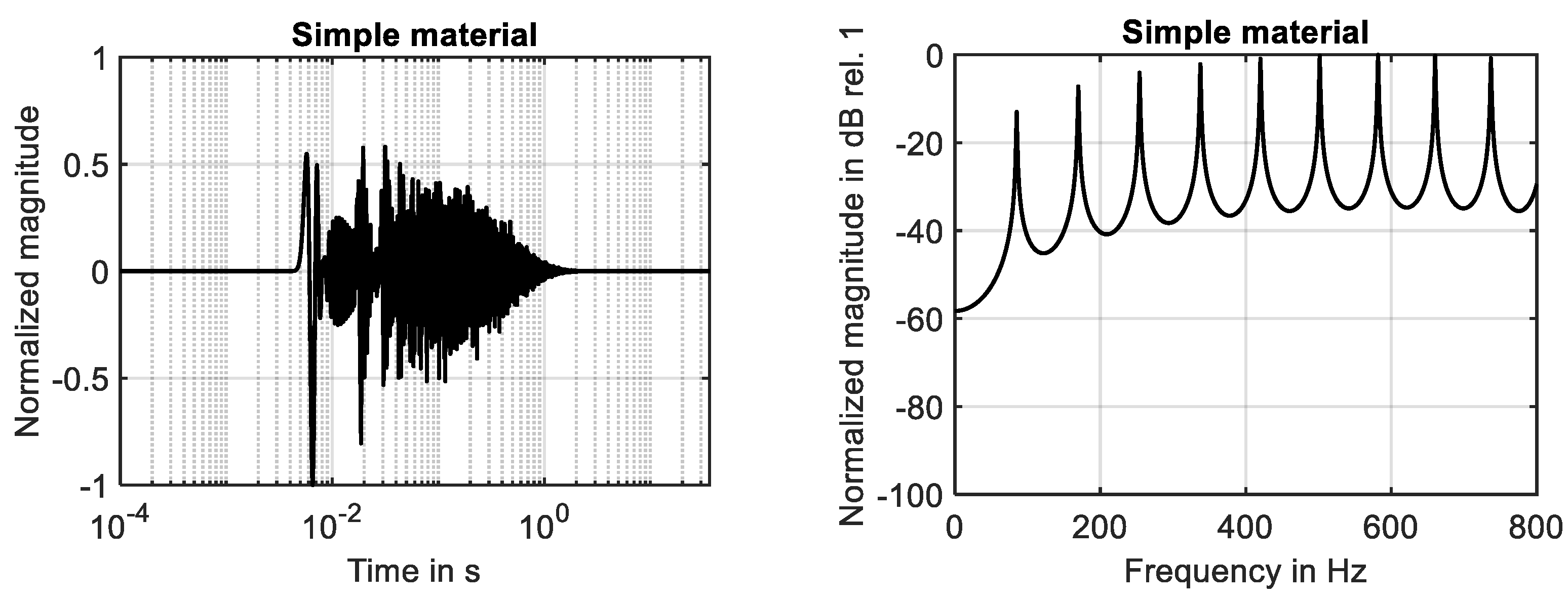
In addition to the boundary condition listed in Equation (21), the damping parameter has been set to $r=0.00005 \mathrm{s}/{\mathrm{m}}^2$. The results of these simulations are shown in Figure 2 and Figure 3 for both time domain and frequency domain. Please note that the curves are normalized to the maximum of the absolute values of the dependent variable.

For both materials, the impulse response decreases rapidly and shows the typical behavior of linear systems with viscous damping. To recognize the differences, it is necessary to compare the frequency response curves shown in Figure 2 (right) and Figure 3 (right). For the simple material, in total, nine resonances can be detected below 800 Hz. As known from the classical theory, these resonances are equally spaced. The results are in full agreement with Equation (10), if higher gradient effects are neglected, i.e., ${\alpha }^4=0$.

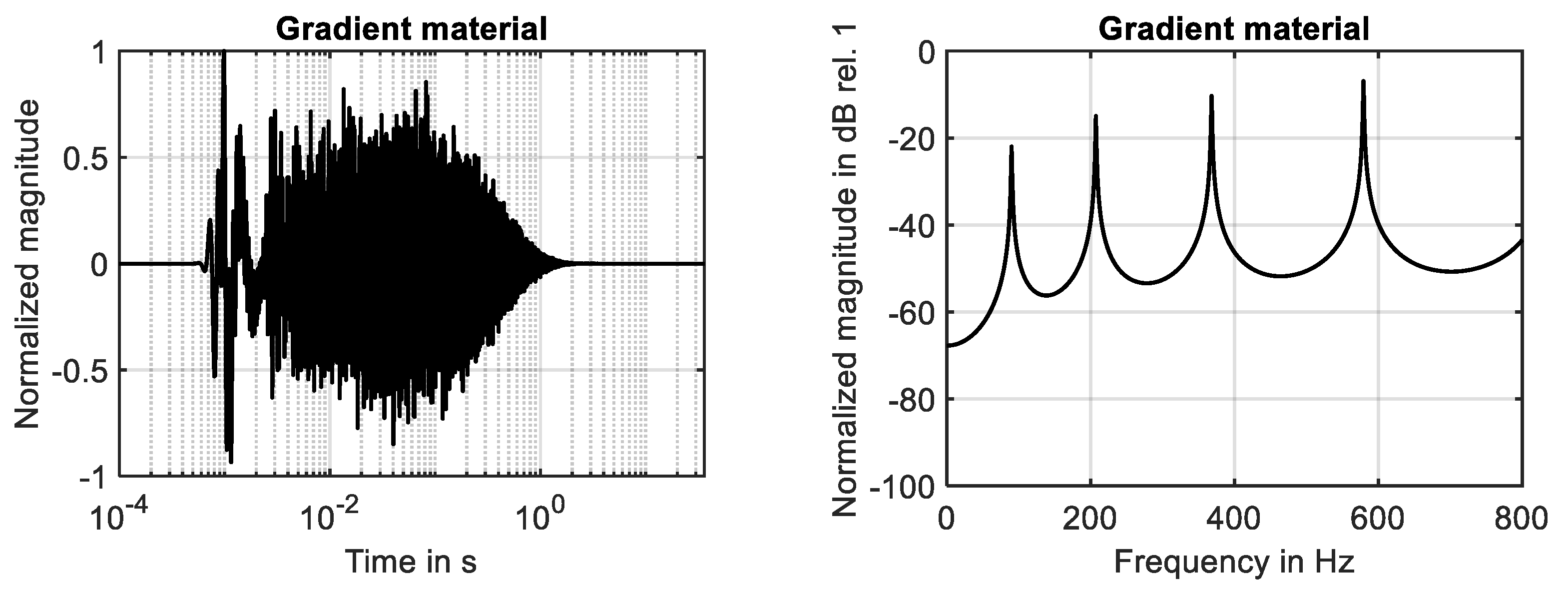
As shown in Figure 3 (right), the number of resonances is reduced down to four if the second-order gradient material is analyzed. The spacing between the resonances increases with an increase in mode number. Furthermore, modes with the same mode number occur at higher frequencies compared to the simple material. Thus, the results of the numerical simulations confirm the analytical solution given in Equation (10), see

Table 2. Comparison of analytical/numerical solution for natural frequencies for a sampling frequency of 85.0 kHz and 31 grid points.

No	Simple Material	Relative Error	Gradient Material	Relative Error
1	85.0 Hz/84.9 Hz	−0.1%	90.1 Hz/90.0 Hz	−0.1%
2	170.0 Hz/169.7 Hz	−0.1%	207.8 Hz/207.3 Hz	−0.2%
3	255.0 Hz/254.1 Hz	−0.4%	370.4 Hz/368.1 Hz	−0.6%
4	340.0 Hz/337.4 Hz	−0.8%	586.3 Hz/579.3 Hz	−1.2%

. Furthermore, it has been found that the relative error between the analytical and numerical results is limited by −1.2% using the discretization in time and space specified in Table 1.

To verify the numerical implementation, the influence of the time step on the relative error was also analyzed. The same applies for the effect of the spatial discretization on the relative error. The associated results are presented in Appendix B. It has been found that the relative error is still limited by −1.2% using sampling frequencies of 42.5 kHz and 170 kHz, if the spatial discretization is not changed, see

Table A1. Comparison of analytical/numerical solution for natural frequencies for a sampling frequency of 42.5 kHz and 31 grid points.

No	Simple Material	Relative Error	Gradient Material	Relative Error
1	85.0 Hz/85.0 Hz	0.0%	90.1 Hz/90.1 Hz	−0.1%
2	170.0 Hz/169.7 Hz	−0.2%	207.8 Hz/207.3 Hz	−0.2%
3	255.0 Hz/254.0 Hz	−0.4%	370.4 Hz/368.3 Hz	−0.6%
4	340.0 Hz/337.5 Hz	−0.7%	586.3 Hz/579.4 Hz	−1.2%

and

Table A2. Comparison of analytical/numerical solution for natural frequencies for a sampling frequency of 170.0 kHz and 31 grid points.

No	Simple Material	Relative Error	Gradient Material	Relative Error
1	85.0 Hz/84.9 Hz	−0.1%	90.1 Hz/90.0 Hz	−0.1%
2	170.0 Hz/169.7 Hz	−0.2%	207.8 Hz/207.2 Hz	−0.3%
3	255.0 Hz/253.9 Hz	−0.4%	370.4 Hz/368.1 Hz	−0.6%
4	340.0 Hz/337.5 Hz	−0.7%	586.3 Hz/579.2 Hz	−1.2%

. It has also been found that the relative error can increase up to 4.7% if the spatial discretization is reduced down to 16 grid points, considering a sampling rate of 85 kHz. However, using 46 grid points, it has also been confirmed that the maximum relative error is reduced down to −1.2% if the spatial discretization is increased, see

Table A3. Comparison of analytical/numerical solution for natural frequencies for a sampling frequency of 85.0 kHz and 16 grid points.

No	Simple Material	Relative Error	Gradient Material	Relative Error
1	85.0 Hz/84.8 Hz	−0.2%	90.1 Hz/89.9 Hz	−0.2%
2	170.0 Hz/168.7 Hz	−0.8%	207.8 Hz/205.7 Hz	−0.9%
3	255.0 Hz/250.0 Hz	−1.7%	370.4 Hz/361.2 Hz	−2.5%
4	340.0 Hz/330.2 Hz	−2.9%	586.3 Hz/558.5 Hz	−4.7%

and

Table A4. Comparison of analytical/numerical solution for natural frequencies for a sampling frequency of 850.0 kHz and 46 grid points.

No	Simple Material	Relative Error	Gradient Material	Relative Error
1	85.0 Hz/85.0 Hz	0.0%	90.1 Hz/90.1 Hz	0.0%
2	170.0 Hz/169.9 Hz	−0.1%	207.8 Hz/207.5 Hz	−0.1%
3	255.0 Hz/254.5 Hz	−0.2%	370.4 Hz/369.4 Hz	−0.3%
4	340.0 Hz/338.3 Hz	−0.5%	586.3 Hz/583.2 Hz	−0.5%

. The computational load is also influenced by the fineness of the time step and the fineness of the spatial discretization. Using an ordinary personal computer, the lowest CPU time (102 s) was determined for the simulation of the simple material using as sampling frequency of 42.5 kHz and a spatial discretization of 16 grid points. The highest CPU time (130 s) was detected during the simulation of the gradient material considering a sampling frequency of 170.0 kHz and 46 grid points.

4.2. Time-Harmonic Excitation

In the second step, adaptive filtering was applied considering time-harmonic excitation with an excitation frequency of $f=150.0 \mathrm{Hz}$ at $x=0$ and a damping parameter of $r=0.00005 \mathrm{s}/{\mathrm{m}}^2$. The associated boundary conditions are summarized in Equation (22)

$$u\left(0,t\right)=\cos \left(2\pi f\cdot t\right) u\left(L,t\right)=0 \frac{{\partial }^{2}u\left(0,t\right)}{\partial x^2}=0 \frac{{\partial }^{2}u\left(L,t\right)}{\partial x^2}=0.$$

(22)

Because adaptive filtering has been performed using a harmonic signal, it has been sufficient to restrict the filter length to $N_w=2$. The minimum power of the reference signal has been set to $P_{\min }=0.0001 \mathrm{V}$, and $\tilde{h}=0.0005$ has been used as the normalized step size.

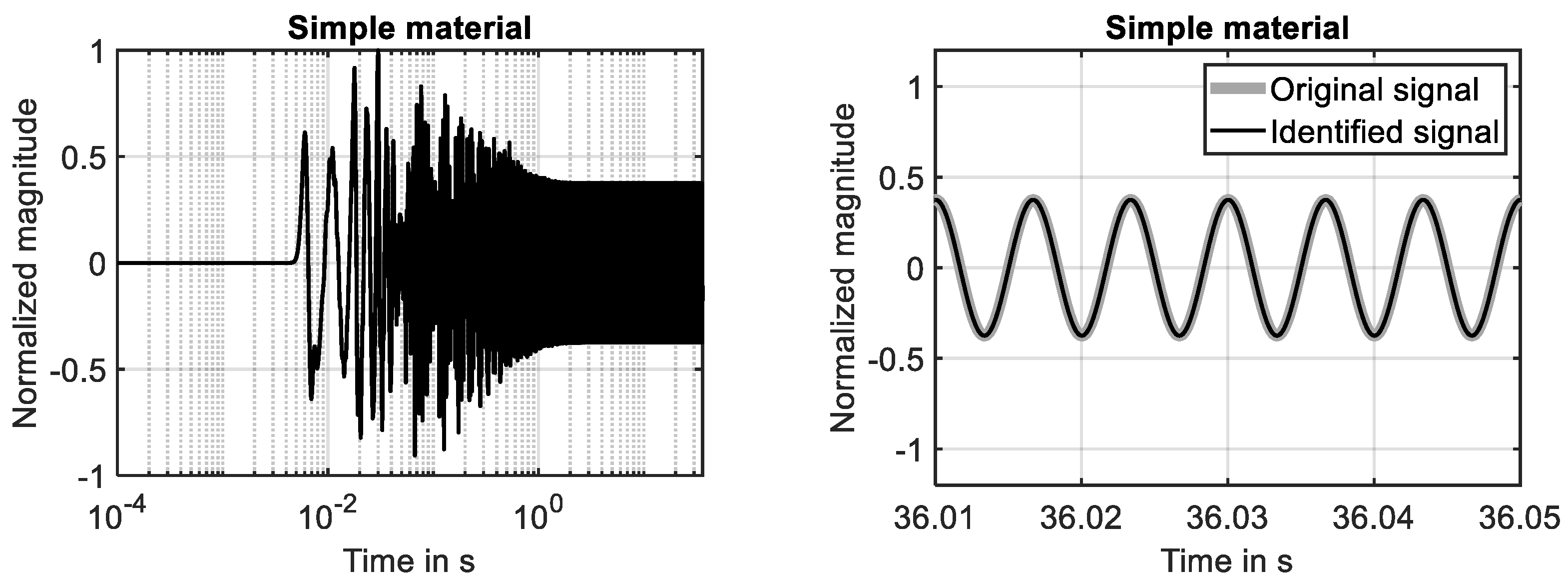
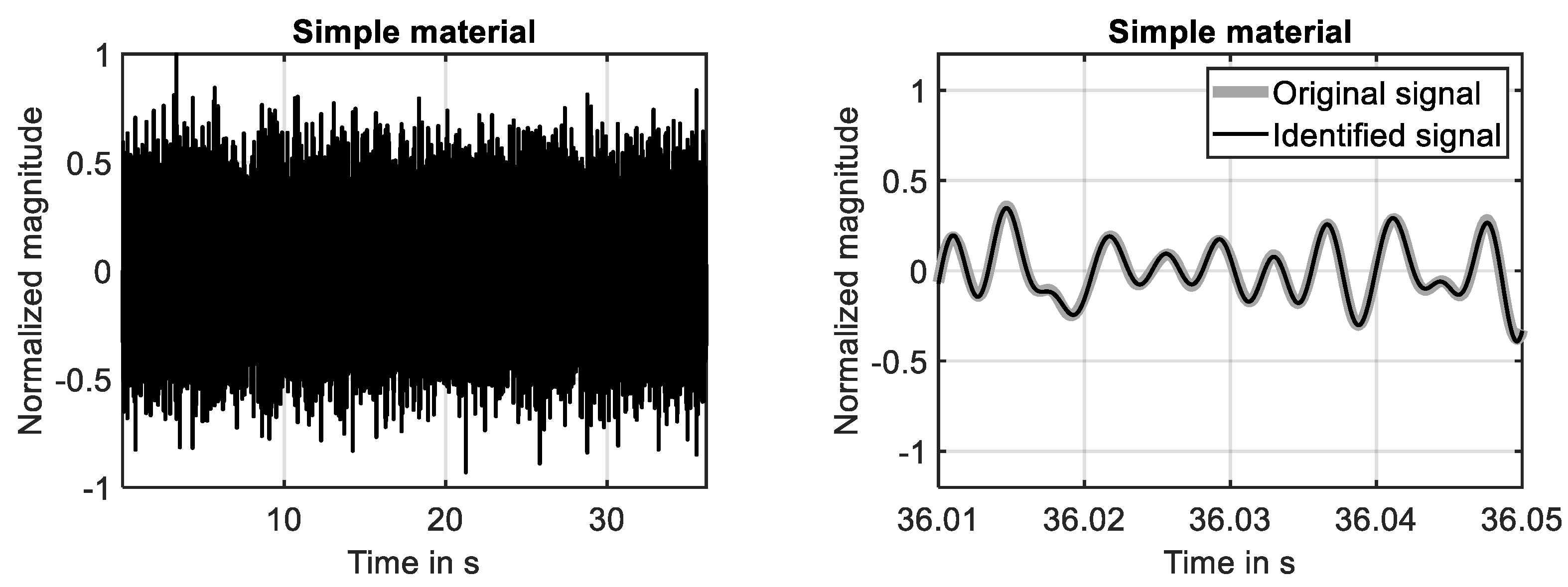
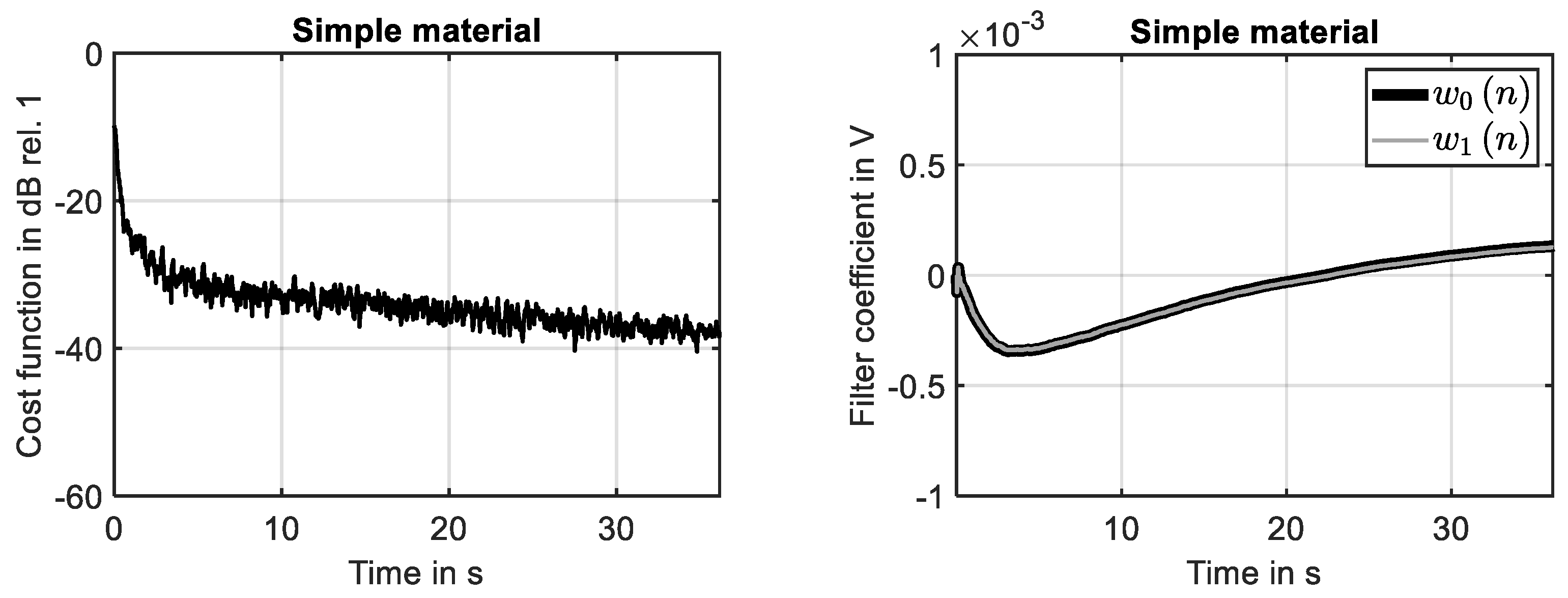
The time-harmonic response of the simple material is shown in Figure 4 (left) for the first ten seconds of the simulation. The steady-state response is fully developed during the first two seconds. This finding is in agreement with the decay of the associated impulse response, see Figure 2 (left). The results shown in Figure 4 (right) clarify that the system response determined at the 29th grid point is fully identified by the adaptive filter. 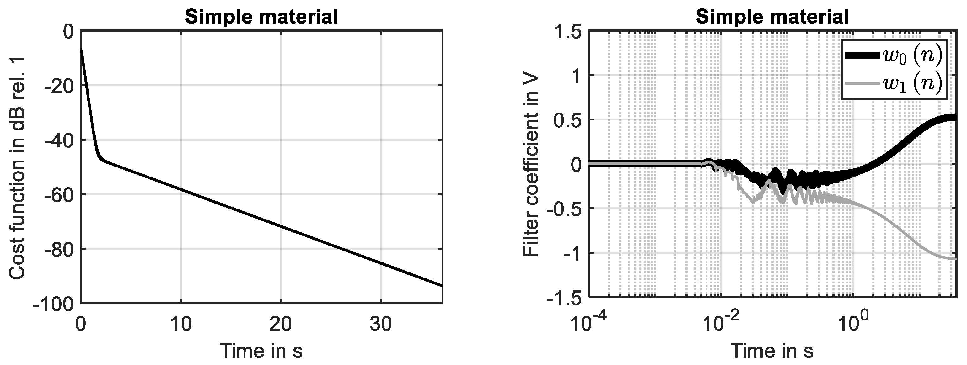The adaption process is illustrated by Figure 5. While the reduction in the cost function (learning curve) is shown in Figure 5 (left), the development of the two filter coefficients is presented in Figure 5 (right). It can been seen that using the NLMS, a rapid convergence of the filter weights has been achieved.

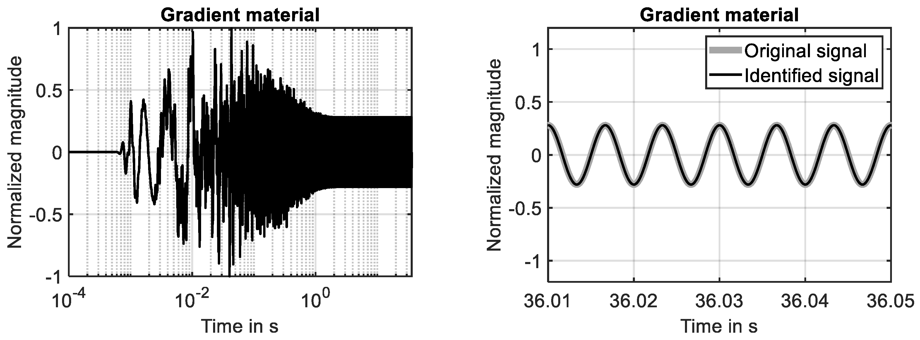
The time-harmonic response of the second-order gradient material is presented in Figure 6 (left), considering again the first ten seconds of the simulation. Also, for this material, the steady-state response is fully developed after the first two seconds. This finding is in agreement with the decay of the associated impulse response. The latter is shown in Figure 3 (left).

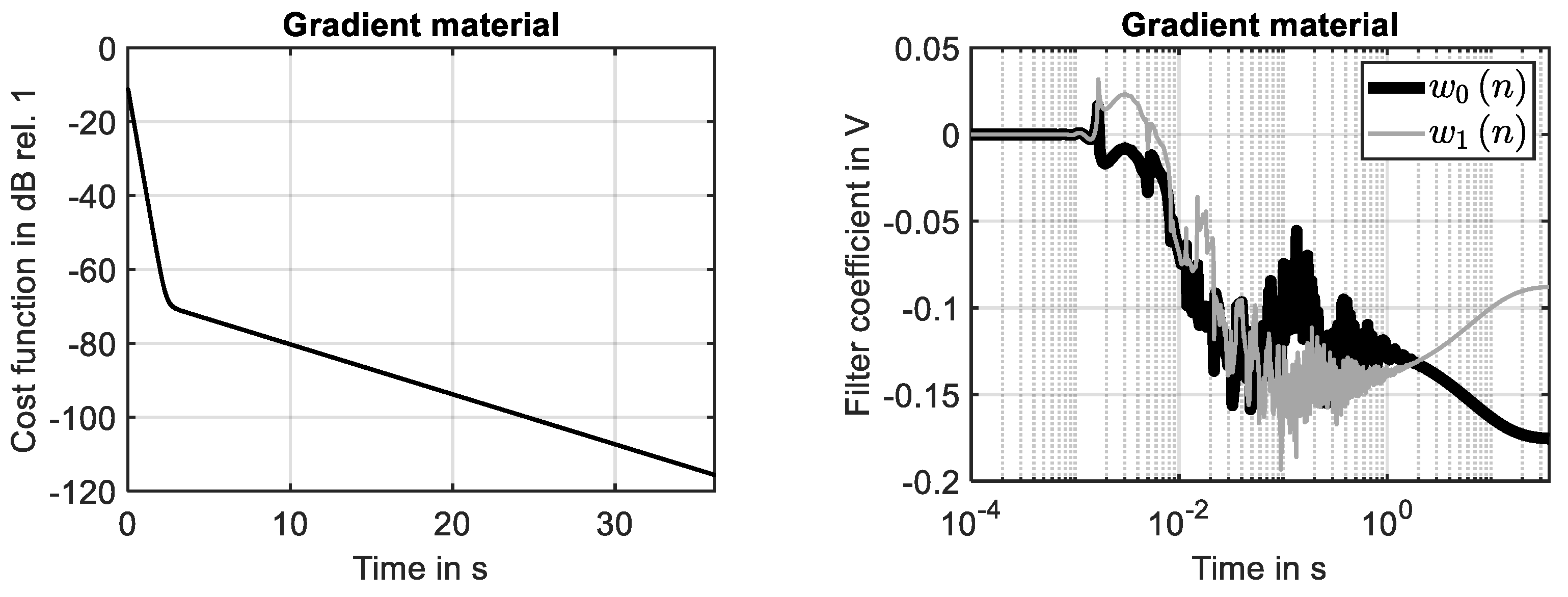
The results shown in Figure 6 (right) prove that the system response determined for the second-order gradient material at the 29th grid point is identified by the adaptive filter with high accuracy. The adaption process is illustrated by Figure 6. The reduction in the cost function, shown in Figure 7 (left), is similar to the learning curve of the simple material, see Figure 5 (left).

The development of the two filter coefficients is presented in Figure 7 (right). As for the simple material, see Figure 5 (right), a fully converged filter is achieved at the end of the simulation. This clarifies that the NLMS algorithm can be applied to identify the time-harmonic response of LTI systems that include higher gradient effects with the same accuracy known for LTI systems based on simple materials.

Please note that it was necessary to increase the filter length or to adjust the normalized step size of the self-adaptive algorithm. The same applies for the minimum reference signal power $P_{\min }$ and the normalized step size $\tilde{h}$. This implies that the same set of parameters that defines the process of adaptive filtering can be used to monitor changes in the material behavior. Because of the differences in the evolution of filter weights, see Figure 5 (right) and Figure 7 (right), it is possible to monitor a change in the material behavior that can be caused by the relevance of higher gradients.

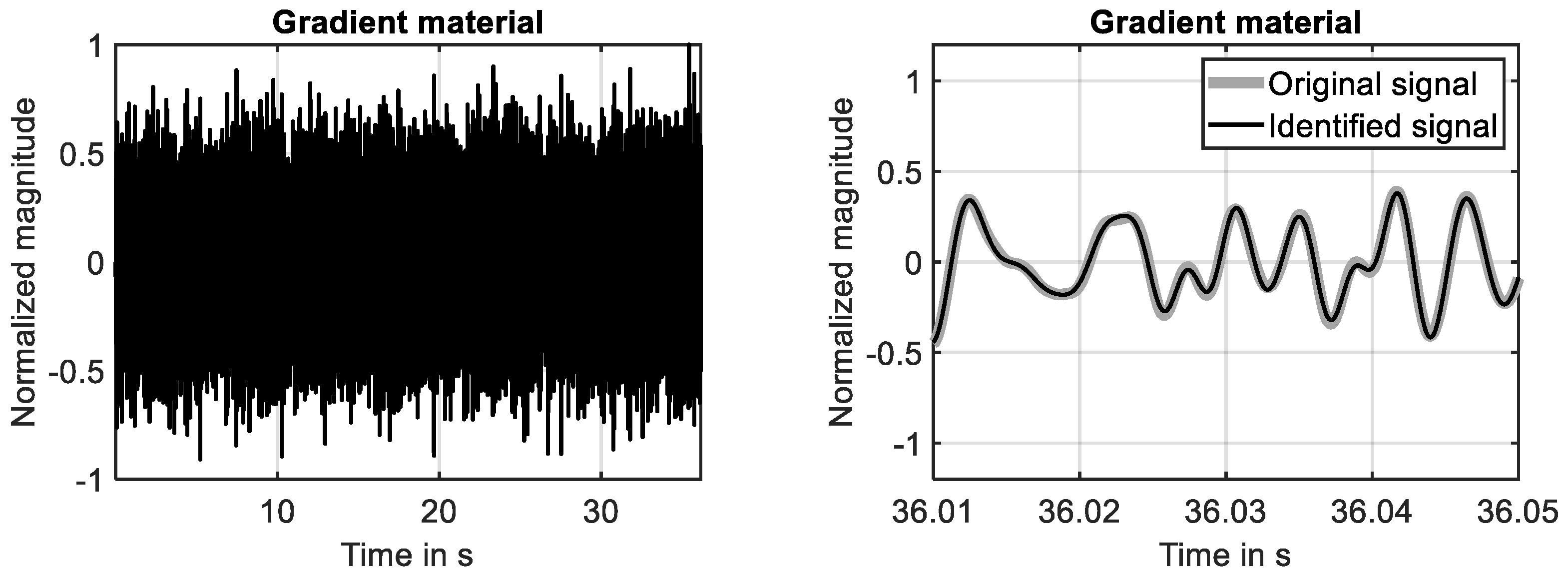
4.3. Band-Limited Noise

In the third step, adaptive filtering was applied considering band-limited Gaussian noise in the frequency range $70.0 \mathrm{Hz}\le f\le 250.0 \mathrm{Hz}$. This reference signal was used to excite the system at the position $x=0$. The damping parameter was increased significantly to $r=0.005 \mathrm{s}/{\mathrm{m}}^2$. The boundary conditions used in this third step are summarized in Equation (23)

$$u\left(0,t\right)=\xi \left(t\right) u\left(L,t\right)=0 \frac{{\partial }^{2}u\left(0,t\right)}{\partial x^2}=0 \frac{{\partial }^{2}u\left(L,t\right)}{\partial x^2}=0,$$

(23)

where $\xi \left(t\right)$ represents the random excitation signal. The length of the adaptive filter was also increased. It was set to $N_w=2048$. The minimum power of the reference signal and the normalized step size were not altered. Thus, the minimum power was again set to $P_{\min }=0.0001 \mathrm{V}$, and $\tilde{h}=0.0005$ was again used as the normalized step size.

For the simple material, the time domain response simulated in the first ten seconds is shown in Figure 8 (left), while the converged state at the end of the simulation is shown in Figure 8 (right). The presented results prove that the system response is identified by high accuracy in the investigated frequency range. This finding is also supported by the learning curve shown Figure 9 (left), because the squared error is reduced down to −40 dB at the end of the simulation. The development of the first two filter weights is shown in Figure 9 (right). It can be seen that these filter weights strive against constant values at the end of the simulation.

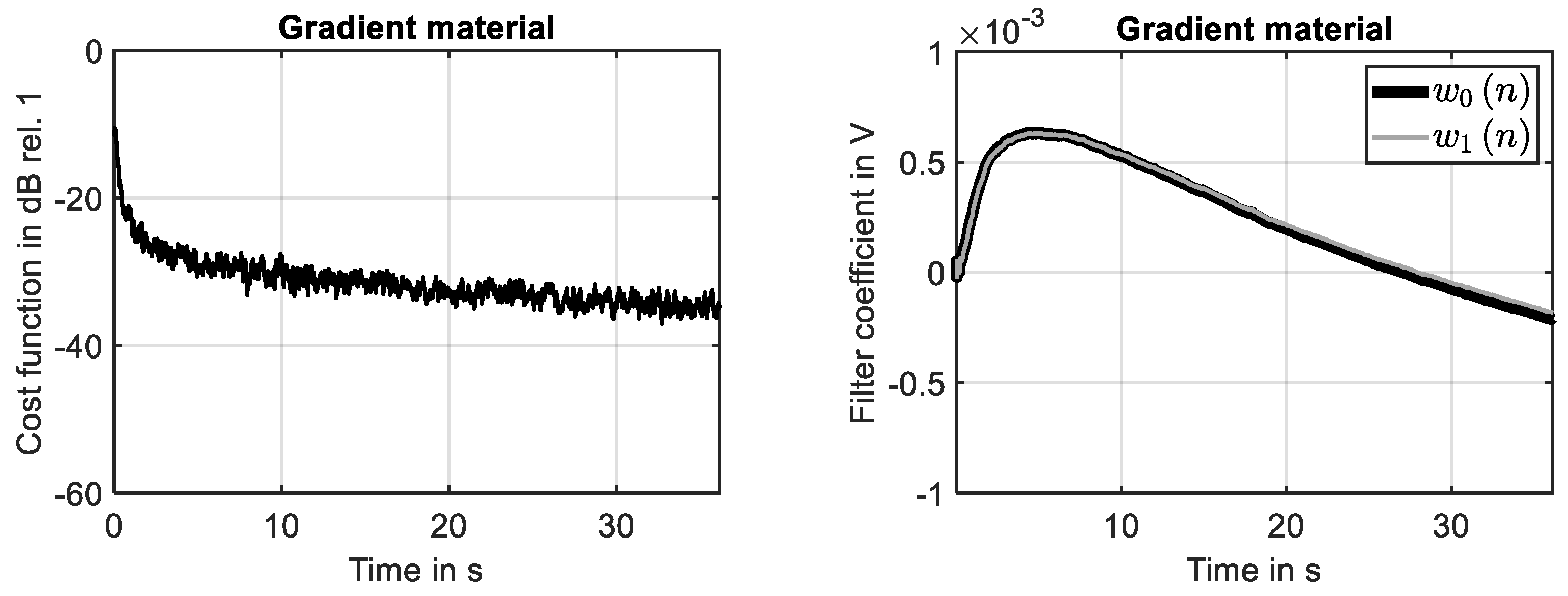
The time domain response of the second-order gradient material simulated in the first ten seconds is shown in Figure 10 (left). As for the simple material, the system is identified with high accuracy at the end of the simulation, see Figure 10 (right). This finding is again supported by the learning curve shown Figure 11 (left), because the squared error is reduced down to −45 dB at the end of the simulation. The development of the first two filter weights is shown in Figure 11 (right). It can be seen that nearly constant values are reached at the end of the simulation.

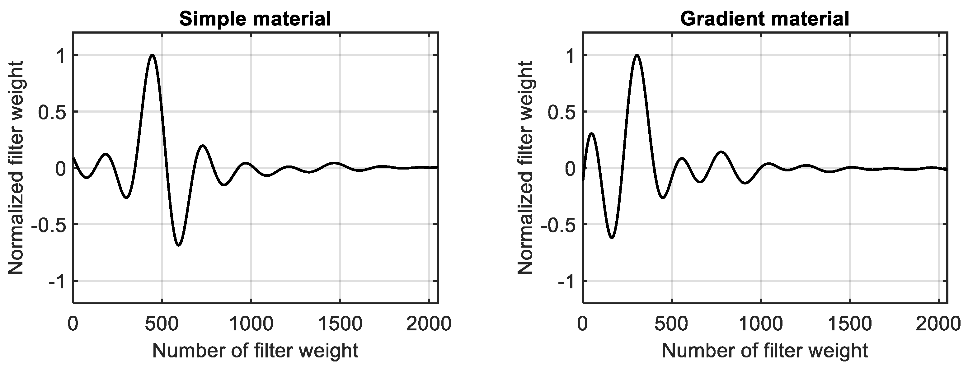
In a converged state, the coefficients of the adaptive filter represent the impulse response of the investigated system in the investigated frequency range. Using a normalization to the maximum of the absolute values, the converged filter coefficients of the simple material are presented in Figure 12 (left). The converged and normalized filter weights that have been identified for the second-order gradient materials are shown in Figure 12 (right). For both materials, a stable impulse response has been identified in the investigated frequency range. Please note that both impulse response curves tend to zero with an increasing filter weight number because viscous damping has been taken into account.

Because different systems based on different material models have been identified, the impulse response curves shown in Figure 12 are not identical. However, as for the time-harmonic signal, the parameters of the adaptive schema have been changed. This opens the possibility of using monitoring techniques such as online plant modeling [34] to observe changes in the system behavior that could be caused by an increase in the relevance of higher gradients in the material behavior. For a practical approach to system identification and condition monitoring, it is possible to formulate the following statements as the main findings of the numerical investigations presented in Section 4:

Statement 1: If the investigated system behaves in a linear and time-invariant way and is fully observable, the influence of higher gradients of the kinematic variables can be relevant for the development of system models, if the number of resonances in a certain frequency band is reduced and the spacing between single resonances increases with an increase in frequency.

Statement 2: If the investigated system behaves in a linear and time-invariant way and is fully observable, a change in the convergence characteristics of the adaptive filter weights that is not caused by changing the parameter of the adaptive schema can indicate a change in the material behavior that can be caused by an increasing relevance of higher-order gradients of the kinematic variables.

Statement 3: If the investigated system behaves in a linear and time-invariant way and is fully observable, a change in the impulse response (that might be observed in condition monitoring during online plant modeling) that is not caused by changing the parameter of the adaptive schema can indicate a change in the material behavior that can be caused by an increasing relevance of higher-order gradients of the kinematic variables.

5. Conclusions

For the first time, system identification based on self-adaptive filtering has been applied to second-order gradient materials using numerical models. These models have been derived from thermodynamically consistent material models that are embedded into a general three-dimensional framework for gradient materials. For this reason, it has not been necessary to consider parameters such as internal length scales that can be used to link the material behavior to a specific internal micro structure. Because of the thermodynamically consistent approach, it has been possible to compare all of the results with the behavior of simple materials.

To obtain simple numerical models, the FDM has been applied. System identification has been performed using the NLMS algorithm. All investigations have been restricted to vibrations in longitudinal finite wave guides. It has been found that in contrast to the classical theory of simple materials, these kind of vibrations are described by a fourth-order PDE. In agreement with the state-of-the-art, it has also been found that such a PDE can be solved analytically for a specific set of boundary conditions. The resulting solution allows for calculating natural frequencies that can differ significantly from the solution known for a simple material.

In particular, it has been found that the influence of second-order gradients of the kinematic variables results in higher values for the natural frequencies and a spacing of natural frequencies that is not equidistant in frequency. The deviation in the natural frequencies increases with an increase in frequency. It starts with a deviation of 6% at the first natural frequency and reaches a deviation of 72.5% at the fourth natural frequency. To observe such a characteristic in a frequency response curve can be relevant for the development of adequate continuum mechanical models. However, all simulations have been validated successfully considering an analytical solution. It has been found that the relative error was reduced down to 0.0% at the first natural frequency using 46 grid points and a sampling frequency of 170 kHz. This holds for both the simple material and the gradient material. It has also been found that the relative error increases if the spatial discretization is reduced. Furthermore, the effect of spatial discretization on the results is more important, compared to the influence of the sampling frequency. Nevertheless, for the lowest spatial discretization (using 16 grid points) in combination with the lowest sampling frequency (42.5 kHz), the absolute value of the relative error did not exceed 4.7% at the fourth natural frequency, considering gradient material behaviour.

The results of the numerical investigation in combination with the adaptive filtering applied for system identification prove that this technique can also be successfully applied to gradient materials. However, compared to simple materials, differences have been found, especially in the evolution of the filter weights. These differences could be used for applications in the field of condition monitoring.

According to the author, future work in this field should include experimental data observed in physical experiments. Furthermore, the field is open to derive more mathematical models that can be used to describe more sophisticated wave propagation phenomena (such as shear waves or bending waves) as well as to develop more advanced numerical models in order to guarantee stable integration schemas. Taking progress in these research directions into account, self-adaptive filtering can become an interesting alternative to other identification methods, especially for dynamical problems. It should also be noticed that the present contribution is limited to small strains and LTI-systems at low frequencies. Thus, the introduction of non-linear effects as well as the discussion of high-frequency effects are open topics for further investigation. Furthermore, only the second gradients of the kinematic variables have been taken into account. For this reason, the introduction of higher gradient terms can also be considered in future investigations.