Orbit Rendezvous Maneuvers in Cislunar Space via Nonlinear Hybrid Predictive Control

Abstract

The NASA’s Artemis project intends to bring humans back to the Moon in the next decade. A key element of the project will be the Lunar Gateway, a space station placed in a peculiar, near rectilinear Halo orbit in the vicinity of a collinear libration point in the Earth–Moon system. This study focuses on the high-fidelity description of the relative orbit dynamics of a chaser spacecraft with respect to the Gateway, as well as on the design of a proper orbit control strategy for rendezvous maneuvers. A novel formulation of the Battin–Giorgi approach is introduced, in which the reference orbit is that traveled by the Gateway, i.e., it is a highly non-Keplerian, perturbed orbit. The modified Battin–Giorgi approach allows for the description of a relative orbit motion with no restrictive assumption, while including all the relevant orbit perturbations on both the chaser and the Gateway. Moreover, nonlinear hybrid predictive control is introduced as a feedback guidance strategy. This new technique is shown to outperform the classical, well-established feedback linearization in terms of success rate and accuracy on the final conditions. Moreover, a Monte Carlo analysis confirms that hybrid predictive control is also effective in the presence of the temporary unavailability of propulsion or thrust misalignment.

1. Introduction

In the context of the NASA Artemis program for lunar exploration, Gateway will play a crucial role. This space station will serve as a permanent advanced logistics outpost, collecting supplies and resources for human missions in the lunar environment and beyond [1]. Gateway will travel a near rectilinear Halo orbit (NRHO) in cislunar space, beneficial for extended communication periods between Gateway and potential future facilities at the lunar South pole. The stability properties of this peculiar orbit were already tested by the CAPSTONE mission [2], while the launch of the first two modules of Gateway are scheduled at the end of 2025.

Designing orbit transfers to and from the Gateway is essential to enable the station’s operations. Various strategies have been explored for both stable and unstable orbits, using underlying manifold structures for optimal departures and approaches. Howell et al. [3] proposed low-cost transfers between the Earth–Moon and Sun–Earth systems using transit orbits. Alessi et al. [4] developed a two-impulse transfer strategy between Low Earth Orbits (LEOs) and Lissajous orbits at two collinear libration points, with the use of the related stable invariant manifold in the dynamical framework of the Circular Restricted 3-Body Problem (CR3BP). A polyhedral representation for invariant manifolds was introduced by Pontani et al., to classify trajectories near the interior collinear libration point and identify optimal low-thrust and two-impulse transfers from LEOs to Lyapunov orbits [5]. More recently, Singh et al. [6] investigated low-thrust transfers to the southern near rectilinear Halo orbit at $L_2$ leveraging invariant manifolds.

Transfer trajectories for stable orbits have been designed using both low-thrust and impulsive maneuvers. More specifically, low-thrust transfers between Distant Retrograde Orbits (DROs) and halo orbits in the Earth–Moon system were obtained by Parish et al. [7], while Pino et al. [8] identified intermediate orbits for low-thrust transfers by exploiting energy surfaces. Pritchett et al. [9] used a collocation algorithm for low-thrust transfers, while Das et al. [10] combined machine learning and numerical optimization for trajectory design, while leveraging dynamical structures. McCarty et al. [11] proposed a monotonic basin hopping optimization technique to find low-thrust transfers from a Gateway-like near rectilinear Halo orbit (NRHO) to a DRO. Additionally, Vutukuri [12] investigated intermediate resonant orbits and their manifolds for transfers between stable orbits, whereas Zimovan et al. [13] utilized higher-period orbits and the related dynamical structures to achieve similar goals.

Low Lunar Orbits (LLOs) are the most convenient parking paths for lunar descent and safe touchdown [14]. In the context of the CR3BP, several studies addressed transfers between Gateway and LLOs. Rozek et al. [15] used an elitist non-dominated sorting genetic algorithm to find two-impulse transfers, further refined by gradient-based optimization. Lu et al. [16] combined local gradient optimization with a numerical continuation strategy to yield optimal direct transfers, while constraining the time of flight to the maximal value of six days. Bucchioni et al. [17] compared Lambert/differential corrections, direct numerical optimization, and Hohmann/differential corrections for similar transfers. Giordano and Topputo [18] focused on the orbit transfers of nanosatellites from LLO to a halo orbit in the presence of uncertainties. Recently, Sanna et al. [19] proposed a fast, minimum-fuel two-impulse transfer strategy suitable for manned missions, incorporating all relevant perturbations in a high-fidelity model. Pozzi et al. [20] also used a high-fidelity dynamical framework to determine minimum-time low-thrust transfers from Gateway to LLO. It is worth remarking that the actual Gateway’s orbit (available from the NAIF kernel [21]) requires modest stationkeeping maneuvers (of a few millimeters per second), to perform at aposelenium, with the intent of avoiding inadvertent departure from the nominal quasi-periodic orbit after a few periods [22]. Related to this aspect, Alvarado and Singh [23] recently proposed an interesting technique for orbit maintenance in the framework of the elliptic restricted three-body problem.

Once a spacecraft has completed its orbit transfer to Gateway, active orbit control is required for successful rendezvous. Numerous studies have addressed rendezvous maneuvers, often assuming that the target spacecraft travels a circular orbit, with the consequent application of linear orbit theory, i.e., the Hill–Clohessy–Wiltshire (HCW) equations of relative orbit motion. Using the latter theoretical framework, Pontani et al. [24] focused on minimum-time and minimum-fuel rendezvous maneuvers. Relative orbit elements were used by Bevilacqua et al. [25] to develop an analytical solution for spacecraft relative orbit control by means of on/off continuous thrusters. Gurfil [26] investigated relative motion between two elliptic Keplerian orbits without linear orbit theory, while Lopez et al. [27] proposed a guidance scheme based on Lyapunov stability theory for impulsive velocity changes. Kluever [28] tackled the same problem with a feedback control scheme capable of yielding the continuous thrust vector along two orthogonal axes. More recently, Karlgaard [29] introduced a guidance strategy using polar coordinates and feedback linearization. The latter technique was also employed by Santoro et al. [30], in conjunction with the Battin–Giorgi description of relative orbit motion, without any linearizing approximation. Nonlinear approaches such as sliding mode control and adaptive control have also been explored for close-range maneuvering. In this context, Anand et al. [31] utilized a nonsingular terminal sliding mode controller based on the HCW equations. Capello et al. [32] and Li et al. [33] also investigated the final phase of rendezvous through sliding mode control.

The aim of this study is the analysis, development, and test of a convenient formulation to model relative orbit motion, together with an effective orbit control strategy for the rendezvous of a spacecraft with Gateway. In particular, a new formulation of the nonlinear BG approach is presented for the description of relative orbit dynamics. Feedback linearization is first applied to orbit rendezvous in cislunar environment. Then, nonlinear hybrid predictive control, i.e., a new feedback guidance strategy for approaching Gateway, is introduced and discussed. Several tests are run in both nominal and nonnominal conditions in order to evaluate the performance of hybrid predictive control.

The paper is organized as follows: In Section 2 a detailed overview of Gateway’s orbit characteristics is offered. In Section 3 the dynamical model employed for the description of the relative motion is presented. The rendezvous strategy is discussed in Section 4, while Section 5 treats the orbit control used to perform the rendezvous maneuver. Tests in both nominal and nonnominal conditions are reported in Section 6 and in Section 7, respectively. Final conclusions are drawn in Section 8.

2. Orbital Motion of Gateway

The reference orbit of Gateway is a southern $L_2$ NRHO. The selection of this specific orbit followed several criteria [34]: (i) an $L_2$ family offers improved visibility of the far side of the Moon for communications with respect to the $L_1$ family [14]; (ii) $L_2$ NRHOs exhibit more advantageous stability properties than $L_1$ NRHOs, which implies lower orbit maintenance requirements [35,36]; (iii) a southern NRHO requires less propellant for returning paths directed toward the Earth’s northern hemisphere; (iv) the southern NRHO provides excellent communications coverage of the lunar South pole, a region of high scientific interest due to large water ice deposits in shadowed craters [37]; (v) the 9:2 Lunar Synodic Resonance (LSR) prevents eclipses due to the Earth [38], which can exceed current hardware limitations. Avoiding Earth shadowing was a primary design goal for this reference orbit, while lunar eclipses, though common, pose no threat because they have short duration (80 min or less). The operational orbit of Gateway has a periselenium radius ranging from 3196 to 3557 km, with an average value of 3366 km, and an average orbital period of 6.562 days.

The Gateway’s ephemeris accounts for perturbing effects from the gravitational fields of the Earth, Sun, and Jupiter, as well as the selenopotential harmonics up to an order and degree of 8. Figure 1 depicts the ephemeris-based Gateway trajectory in the Earth–Moon synodic frame.

3. Relative Orbit Dynamics

Successful rendezvous maneuvers require a high-fidelity description of the spacecraft motion relative to Gateway. In this framework, the spacecraft, also referred to as the chaser, approaches Gateway, termed the target. Several approaches to describe relative motion were developed. Linear orbit theory, i.e., the Eulero–Hill equations [39], is commonly used. These methods are based on the linearization of the relative motion equations around the position of the target. For this reason, they provide an accurate description of the motion only when the chaser is sufficiently close to the target. An interesting alternative option is represented by the BG approach. It does not require any linearization, therefore there exist no constraints on the relative distance $\rho$. The classical BG approach describes the motion of a perturbed spacecraft with respect to a reference body on a Keplerian orbit. Hence, in order to obtain the relative motion of the chaser with respect to the target, one should study, separately, the relative motion of target and chaser with respect to a virtual reference body, which travels a Keplerian orbit. The difference of the two relative positions describes the nonlinear relative motion of the chaser with respect to the target. However, because the target travels a highly non-Keplerian path, recurrent updates of the reference Keplerian path are required, and the approach at hand reveals to be rather impratical. In the following, a new formulation of BG method is proposed, where the reference orbit is non-Keplerian. This allows for a more straightforward description of the motion of the spacecraft with respect to Gateway.

In a generic inertial reference frame, the target acceleration is

$${\ddot{\overrightarrow{r}}}_t=-{\displaystyle \frac{\mu }{r_t^3}}{\overrightarrow{r}}_t+{\overrightarrow{a}}_{p,t}$$

(1)

where

• ${\overrightarrow{r}}_t$ indicates the inertial position vector of the target, $r_t=\left|{\overrightarrow{r}}_t\right|$;
• $\mu$ represents the gravitational parameter of the main attracting body (i.e., the Moon);
• ${\overrightarrow{a}}_{p,t}$ is the sum of all the relevant perturbing accelerations acting on the target.

In a similar way, for the chaser

$${\ddot{\overrightarrow{r}}}_c=-{\displaystyle \frac{\mu }{r_c^3}}{\overrightarrow{r}}_c+{\overrightarrow{a}}_{p,c}+{\overrightarrow{a}}_{t,c}$$

(2)

where

• ${\overrightarrow{r}}_c$ indicates the inertial position vector of the chaser, $r_c=\left|{\overrightarrow{r}}_c\right|$;
• ${\overrightarrow{a}}_{p,c}$ is the sum of all the relevant perturbing accelerations acting on the chaser;
• ${\overrightarrow{a}}_{t,c}$ represents the thrust acceleration of the chaser.

The relative position is defined as $\overrightarrow{\rho }={\overrightarrow{r}}_c-{\overrightarrow{r}}_t$, thus $\ddot{\overrightarrow{\rho }}={\ddot{\overrightarrow{r}}}_c-{\ddot{\overrightarrow{r}}}_t$. Considering Equations (1) and (2), $\ddot{\overrightarrow{\rho }}$ can be expressed as

$$\ddot{\overrightarrow{\rho }}=-{\displaystyle \frac{\mu }{r_c^3}}{\overrightarrow{r}}_c+{\displaystyle \frac{\mu }{r_t^3}}{\overrightarrow{r}}_t+{\overrightarrow{a}}_{p,c}+{\overrightarrow{a}}_{t,c}-{\overrightarrow{a}}_{p,t}$$

(3)

Moreover, because ${\overrightarrow{r}}_c=\overrightarrow{\rho }+{\overrightarrow{r}}_t$,

$$\begin{array}{cc}\hfill \ddot{\overrightarrow{\rho }}& =-{\displaystyle \frac{\mu }{r_c^3}}\overrightarrow{\rho }-{\displaystyle \frac{\mu }{r_c^3}}{\overrightarrow{r}}_t+{\displaystyle \frac{\mu }{r_t^3}}{\overrightarrow{r}}_r+{\overrightarrow{a}}_{p,c}+{\overrightarrow{a}}_{t,c}-{\overrightarrow{a}}_{p,t}\hfill \\ \hfill & ={\displaystyle \frac{\mu }{r_t^3}}{\overrightarrow{r}}_t\left[1-{\displaystyle \frac{r_t^3}{r_c^3}}\right]-{\displaystyle \frac{\mu }{r_c^3}}\overrightarrow{\rho }+{\overrightarrow{a}}_{p,c}+{\overrightarrow{a}}_{t,c}-{\overrightarrow{a}}_{p,t}\hfill \\ \hfill & ={\displaystyle \frac{\mu }{r_t^3}}{\overrightarrow{r}}_t\left[1-{\displaystyle \frac{r_t^3}{|\overrightarrow{\rho }+{\overrightarrow{r}}_t{|}^3}}\right]-{\displaystyle \frac{\mu }{r_c^3}}\overrightarrow{\rho }+{\overrightarrow{a}}_{p,c}+{\overrightarrow{a}}_{t,c}-{\overrightarrow{a}}_{p,t}\hfill \\ \hfill & ={\displaystyle \frac{\mu }{r_t^3}}{\overrightarrow{r}}_t\left[1-{\displaystyle \frac{r_t^3}{{\left({\rho }^2+r_t^2+2\overrightarrow{\rho }·{\overrightarrow{r}}_t\right)}^{3/2}}}\right]-{\displaystyle \frac{\mu }{r_c^3}}\overrightarrow{\rho }+{\overrightarrow{a}}_{p,c}+{\overrightarrow{a}}_{t,c}-{\overrightarrow{a}}_{p,t}\hfill \end{array}$$

(4)

Introducing the parameter

$$q={\displaystyle \frac{{\rho }^2+2\overrightarrow{\rho }·{\overrightarrow{r}}_t}{r_t^2}}$$

(5)

the preceding equation becomes

$$\ddot{\overrightarrow{\rho }}={\displaystyle \frac{\mu }{r_t^3}}{\displaystyle \frac{q\left[2+q+{(1+q)}^{1/2}\right]}{{(1+q)}^{3/2}\left[{(1+q)}^{1/2}+1\right]}}{\overrightarrow{r}}_t-{\displaystyle \frac{\mu }{r_c^3}}\overrightarrow{\rho }+{\overrightarrow{a}}_{p,c}+{\overrightarrow{a}}_{t,c}-{\overrightarrow{a}}_{p,t}$$

(6)

In the previous relation, $\ddot{\overrightarrow{\rho }}$ is expressed in an inertial reference frame. Anyway, for relative motion, the Local Horizontal Local Vertical (LVLH) frame centered on the target is preferred with respect to an inertial frame. The axes of this reference system are defined as follows:

• $\widehat{r}$ is parallel to the position vector of the spacecraft with respect to the main body, i.e., the Moon;
• $\widehat{h}$ is parallel to the spacecraft angular momentum;
• $\widehat{\theta }$ completes the right-hand triad.

However, since the LVLH frame is rotating, one has to take into account the transport theorem

$${}^N\dot{\overrightarrow{\rho }}={}^R\dot{\overrightarrow{\rho }}+{}^N\overrightarrow{\omega }^R\times \overrightarrow{\rho }$$

(7)

where ${}^N\dot{\overrightarrow{\rho }}$ and ${}^R\dot{\overrightarrow{\rho }}$ indicate the time derivatives of the relative position with respect to the inertial and the rotating LVLH frame, respectively, while ${}^N\overrightarrow{\omega }^R$ represents the angular velocity of the LVLH frame with respect to the inertial frame. Applying the transport theorem two times yields

$$\begin{array}{cc}\hfill {}^N\ddot{\overrightarrow{\rho }}=& {}^R\ddot{\overrightarrow{\rho }}+2{}^N\overrightarrow{\omega }^R\times {}^R\dot{\overrightarrow{\rho }}+{}^N\dot{\overrightarrow{\omega }}^R\times \overrightarrow{\rho }\hfill \\ \hfill +& {}^N\overrightarrow{\omega }^R\times {}^N\overrightarrow{\omega }^R\times {}^R\dot{\overrightarrow{\rho }}\hfill \end{array}$$

(8)

Comparing Equation (6) with Equation (8), one obtains the final expression of $\ddot{\overrightarrow{\rho }}$ in the LVLH frame,

$$\begin{array}{cc}\hfill \ddot{\overrightarrow{\rho }}=& -2\overrightarrow{\omega }\times \dot{\overrightarrow{\rho }}-\dot{\overrightarrow{\omega }}\times \overrightarrow{\rho }-\overrightarrow{\omega }\times \overrightarrow{\omega }\times \overrightarrow{\rho }\hfill \\ \hfill & +{\displaystyle \frac{\mu }{r_t^3}}{\displaystyle \frac{q\left[2+q+{(1+q)}^{1/2}\right]}{{(1+q)}^{3/2}\left[{(1+q)}^{1/2}+1\right]}}{\overrightarrow{r}}_t-{\displaystyle \frac{\mu }{r_c^3}}\overrightarrow{\rho }+{\overrightarrow{a}}_{p,c}+{\overrightarrow{a}}_{t,c}-{\overrightarrow{a}}_{p,t}\hfill \end{array}$$

(9)

In the last equation, superscripts are neglected for simplicity; the same choice is adopted in the following. For the sake of clarity, all time derivatives are expressed in the rotating LVLH frame, while $\overrightarrow{\omega }$ and $\dot{\overrightarrow{\omega }}$ represent the angular velocity and acceleration, respectively, of the LVLH frame with respect to the inertial frame. The angular velocity can be computed at any desired time from the instantaneous Classical Orbit Elements (COE) of the target [40],

$$\overrightarrow{\omega }={\left(\begin{array}{c}\dot{\Omega }sinisin{\theta }_t+\dot{i}cos{\theta }_t\\ \dot{\Omega }sinicos{\theta }_t-\dot{i}sin{\theta }_t\\ \dot{\Omega }cosi+{\dot{\theta }}_t\end{array}\right)}^T\left(\begin{array}{c}\widehat{r}\\ \widehat{\theta }\\ \widehat{h}\end{array}\right)$$

(10)

where

• $\Omega$ represents the Right Ascension of the Ascending Node (RAAN),
• i indicates the orbit inclination, and
• ${\theta }_t=\omega +\nu$ is the argument of latitude, with $\omega$ and $\nu$ denoting the argument of periapse and true anomaly, respectively.

The time derivatives of COE are provided by the Gauss Variational Equations; in particular $\dot{i}$, $\dot{\Omega }$, and ${\dot{\theta }}_t$ are described by the following formulae [40]:

$$\begin{array}{cc}\hfill \dot{i}& =r{\displaystyle \frac{cos{\theta }_t}{h}}{a}_h\hfill \\ \hfill \dot{\Omega }& =r{\displaystyle \frac{sin{\theta }_t}{hsini}}{a}_h\hfill \\ \hfill {\dot{\theta }}_t& =\sqrt{{\displaystyle \frac{\mu }{p^3}}}{(1+ecos\nu )}^2-r{\displaystyle \frac{sin{\theta }_{t}cosi}{hsini}}{a}_h\hfill \end{array}$$

(11)

with $\left(a_r,a_{\theta },a_h\right)$ being the components of the total perturbing acceleration acting on the target, expressed in the LVLH frame. The angular acceleration $\dot{\overrightarrow{\omega }}$ can be computed in a numerical way. In particular, the target orbital motion is forward propagated for the time interval of interest, by integrating the dynamic equations of the Modified Equinoctial Elements (MEE). Then, Equation (10) is employed to obtain the components of $\overrightarrow{\omega }$. The time histories of each component are interpolated through a cubic spline, whose time derivative leads to the computation of the components of $\dot{\overrightarrow{\omega }}$. The spline and its derivative are carried out with the MATLAB functions spline and fnder, respectively.

The perturbations included in Equations (9) and (11) and in the dynamic equations of MEE are represented by the higher harmonics of the selenopotential and the third-body gravitational perturbation due to the Earth and the Sun [19]. In particular, all the harmonics with coefficients $|J_{l,m}|>5·{10}^{-6}$ are included in the dynamical model.

It is worth noticing that in this model only the target state and the relative motion of the chaser are propagated. In fact, the positions of the Earth and the Sun with respect to the spacecraft are provided by the NAIF ephemeris. The initial position and velocity of Gateway are retrieved from ephemeris data as well.

The main differences introduced with respect to the classical BG scheme depend on the fact that in this formulation the reference orbit is the real path traveled by Gateway, which considers the perturbations that affect it. In particular

• the expressions of $\overrightarrow{\omega }$ and $\dot{\overrightarrow{\omega }}$ take the time variations of COE into account, unlike the case of unperturbed Keplerian motion;
• the target perturbing acceleration ${\overrightarrow{a}}_{p,t}$ is also explicitly included in Equation (6).

The introduction of this high-fidelity framework is fundamental for the study of the motion of the spacecraft relative to Gateway, because the orbit of the latter is strongly perturbed. In fact, any simplifying assumption regarding the target orbit, e.g., considering it as Keplerian or even circular (as in the Eulero–Hill approach), would yield unacceptable inaccuracies.

4. Rendezvous Strategy

The rendezvous maneuver of the space vehicle toward Gateway is studied in the LVLH frame. In particular, the new version of the BG method, explained in detail in Section 3, is employed. Gateway is assumed to be passive, therefore the entire maneuver is performed by the chaser. At the starting time, an initial relative distance $\rho =1.5$ km is considered. The rendezvous is designed as a maneuver with specified duration set to 12 h. Gateway is modeled as a sphere with radius of 5 m. Moreover, the docking port is assumed to be aligned with $\widehat{r}$. Therefore, the desired final relative position, expressed in the target LVLH frame, is

$${\underline{\rho }}_f=\left(\begin{array}{c}5\\ 0\\ 0\end{array}\right)\mathrm{m}$$

(12)

At the same time, for the purpose of performing a smooth docking, the following final relative velocity is selected (in the LVLH frame):

$${\underline{\dot{\rho }}}_f=-\left(\begin{array}{c}1\\ 0\\ 0\end{array}\right){\displaystyle \frac{\mathrm{cm}}{\mathrm{s}}}$$

(13)

The chaser propulsion system consists of a low-thrust engine, characterized by an effective exhaust velocity $c=30{\displaystyle \frac{\mathrm{km}}{\mathrm{s}}}$ and a maximum thrust acceleration $u_{max}=5\times {10}^{-5}{g}_0=4.90310\times {10}^{-4}{\displaystyle \frac{\mathrm{m}}{\mathrm{s}}}$, where $g_0$ represents the gravitational acceleration on Earth at sea level.

In most cases, the role of the propulsion system is in reducing the relative velocity of the spacecraft with respect to Gateway, starting from the dynamical conditions at the end of an orbit transfer. This means that the plume might be pointed toward Gateway at the end of the rendezvous maneuver, which represents a possible threat for the integrity of the lunar station. Moreover, an attitude maneuver is usually necessary in the last meters before mating, in order to align the docking port of the chaser with that of Gateway. To allow this, the last 5 m of the rendezvous maneuver are assumed to be traveled in the absence of propulsion, in a phase termed natural drift. In light of this, when the approaching spacecraft reaches a distance of 10 m from Gateway, low-thrust propulsion is turned off and natural drift begins. For this reason, identifying a suitable dynamical state (i.e., position and velocity) of the chaser at 10 m from Gateway appears crucial. To find this specific state at 10 m from Gateway, the desired final state at docking is backward propagated until the distance reaches 10 m, while assuming no propulsion acceleration in Equation (9). The dynamical state at 10 m from Gateway represents the final target state of relative orbital control, which drives the spacecraft in the thrusted phase. In the next sections, the dynamical state obtained at the end of the powered phase is propagated in the high-fidelity model until the final distance of 5 m is reached, to obtain the outcome of rendezvous at the end of natural drift, even in the presence of nonnominal flight conditions.

5. Feedback Control Techniques

At the end of the orbit transfer directed toward Gateway, the target is in the proximity of the lunar space station, with a certain relative velocity. At this stage, in order to perform a successful rendezvous, an active orbital control that drives the position and velocity of the spacecraft toward the desired ones is crucial. In this study, orbit control for the final approach is based on feedback linearization. Moreover, the limits of classical feedback linearization are discussed and an advantageous modification of this control scheme is presented. An improved feedback orbit control is employed in the rendezvous maneuvers investigated in this work.

5.1. Feedback Linearization

According to Equation (9), the relative dynamics of the chaser with respect to Gateway can be written as

$$\ddot{\underline{\rho }}=\underline{f}+\underline{u}$$

(14)

where $\underline{f}$ represents the natural relative dynamics, while $\underline{u}$ indicates the chaser thrust acceleration. In particular,

$$\begin{array}{cc}\hfill \underline{f}=& -2\underline{\omega }\times \dot{\underline{\rho }}-\dot{\underline{\omega }}\times \underline{\rho }-\underline{\omega }\times \underline{\omega }\times \underline{\rho }\hfill \\ \hfill & +{\displaystyle \frac{\mu }{r_t^3}}{\displaystyle \frac{q\left[2+q+{(1+q)}^{1/2}\right]}{{(1+q)}^{3/2}\left[{(1+q)}^{1/2}+1\right]}}{\underline{r}}_t-{\displaystyle \frac{\mu }{r_c^3}}\underline{\rho }+{\underline{a}}_{p,c}-{\underline{a}}_{p,t}\hfill \end{array}$$

(15)

The desired relative path, associated with ${\underline{\rho }}_d\left(t\right)$ and subscript d, is computed using a cubic spline for each position component. Let subscript f stand for final. These spline functions connect the initial relative position coordinates to the final desired position coordinates, while also enforcing ${\dot{\underline{\rho }}}_d\left(t_f\right)={\dot{\underline{\rho }}}_f$. Once the interpolating spline is identified, ${\dot{\underline{\rho }}}_d\left(t\right)$ and ${\ddot{\underline{\rho }}}_d\left(t\right)$ are obtained as the first and second time derivative of ${\underline{\rho }}_d\left(t\right)$, respectively. The spline is computed by means of the MATLAB spline function, while its time derivatives are computed with MATLAB fnder function. The state error is defined as

$$\underline{E}:=\underline{\rho }-{\underline{\rho }}_d$$

(16)

The thrust acceleration needed to drive the spacecraft toward the desired state is computed as

$$\underline{u}=-\underline{f}+{\ddot{\underline{\rho }}}_d-K_d\left(\dot{\underline{E}}\right)-K_p\left(\underline{E}\right)$$

(17)

where $K_p$ and $K_d$ are the proportional and derivative gain matrices, respectively. After substituting Equation (17) in Equation (14), a second order error equation is obtained

$$\ddot{\underline{E}}+K_d\dot{\underline{E}}+K_p\underline{E}=0$$

(18)

The gain matrices are constant and positive definite. Moreover, they are assumed to be diagonal, with equal postive elements

$$K_p=\left[\begin{array}{ccc}{k}_p& 0& 0\\ 0& k_p& 0\\ 0& 0& k_p\end{array}\right],K_d=\left[\begin{array}{ccc}{k}_d& 0& 0\\ 0& k_d& 0\\ 0& 0& k_d\end{array}\right]$$

(19)

Given the diagonal structure of the gain matrices, Equation (18) corresponds to three uncoupled scalar equations in the form

$${\ddot{e}}_i+k_d{\dot{e}}_i+k_p{e}_i=0,i=r,\theta ,h$$

(20)

This last equation, as any linear second-order differential equation with constant coefficients, can be rewritten in terms of damping ratio $\zeta$ and natural frequency ${\omega }_n$ [41]

$$\begin{array}{cc}\hfill k_p& ={\omega }_n^2\hfill \\ \hfill k_d& =2\zeta {\omega }_n\hfill \end{array}$$

(21)

The two coefficients $k_d$ to $k_p$ can be related by imposing the critical damping condition [41], i.e., $\zeta =1$. Unlike the underdamped ($\zeta <1$) condition, critical damping assures convergence toward the desired state without an oscillatory transient, with a convergence time that is shorter than any overdamped ($\zeta >1$) system. In critical damping regime,

$$k_d=2\sqrt{k_p}$$

(22)

By introducing the vector coefficients

$$\begin{array}{cc}\hfill \underline{a}& =-\underline{f}+{\ddot{\underline{\rho }}}_d\hfill \\ \hfill \underline{b}& =2\left(\dot{\underline{\rho }}-{\dot{\underline{\rho }}}_d\right)\hfill \\ \hfill \underline{c}& =\underline{\rho }-{\underline{\rho }}_d\hfill \end{array}$$

(23)

the norm of the thrust acceleration can be expressed as a function of their components in the target LVLH frame,

$$u=|\underline{u}|=\left|\underline{a}-\sqrt{K_p}\underline{b}-K_p\underline{c}\right|$$

(24)

Using the auxiliary variable $k=\sqrt{k_p}$ and requiring $u=u_{max}$, Equation (24) can be rearranged as

$$|\underline{c}{|}^2{k}^4+2{\underline{b}}^T\underline{c}{k}^3+(|\underline{b}{|}^2-2{\underline{a}}^T\underline{c})k^2-2{\underline{a}}^T\underline{b}k+{\left|\underline{a}\right|}^2-u_{max}^2=0$$

(25)

At any time t, all the quantities $\underline{a}$, $\underline{b}$ and $\underline{c}$ are known. Therefore, this fourth-degree equation for k can be solved at the initial time, and the value of k is found. Finally, $k_p$ is obtained from k as $k_p=k^2$. Only a real positive value of $k_p$ can lead to the convergence of the actual state to desired one. Thus, only real positive solutions of Equation (25) are regarded acceptable. If multiple real positive solutions exist, then the one with the minimum magnitude is selected.

In short, this procedure allows for the finding the value of $k_p$, such that

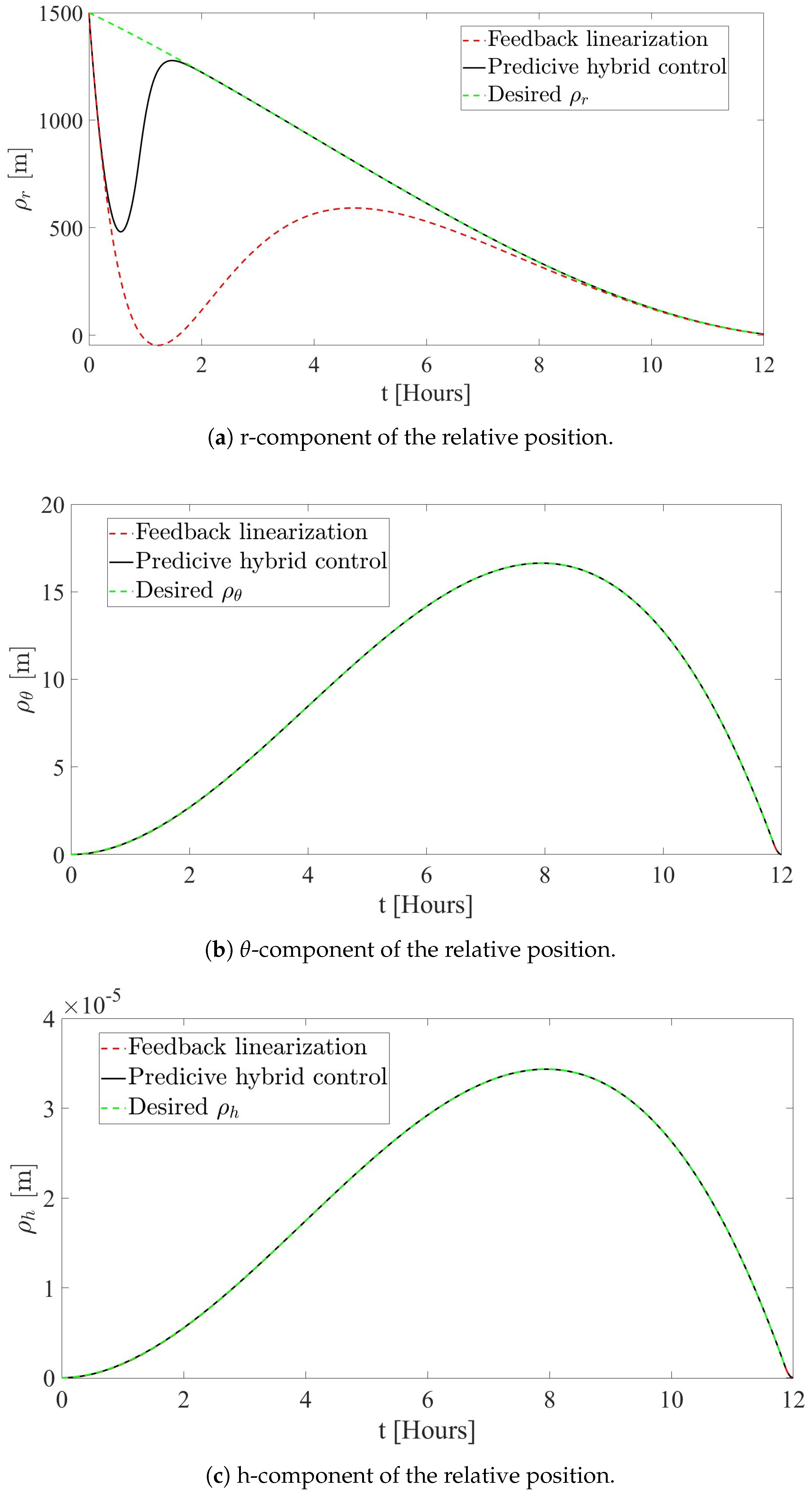
• error components show a critical damping behavior, with convergence toward the desired values, without the occurrence of overshooting;
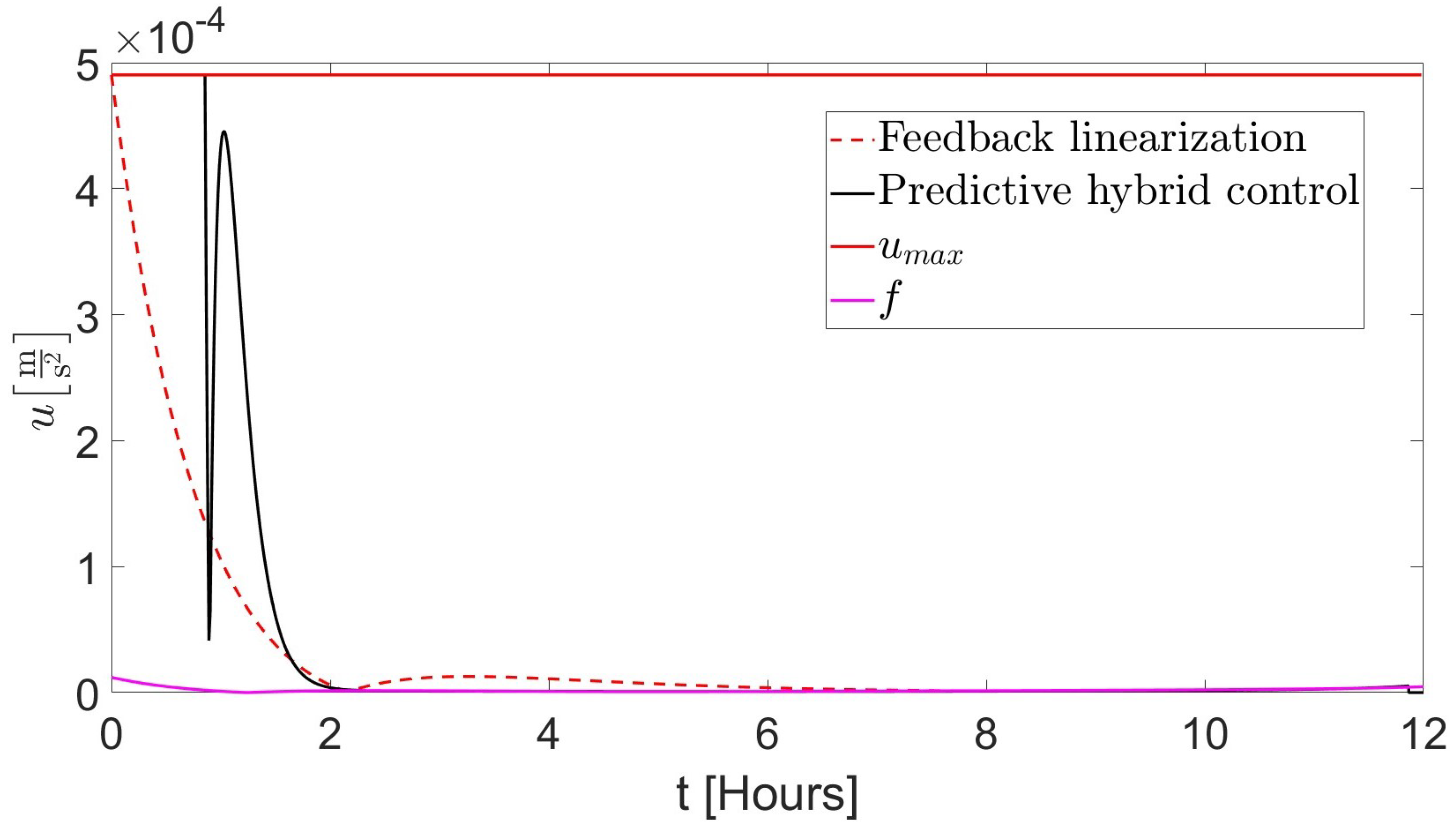
• the initial thrust acceleration magnitude is exactly equal to the maximum available value.

Coefficients $\underline{a}$, $\underline{b}$ and $\underline{c}$ are computed at the beginning of the rendezvous. In this way, Equation (25) can be employed in order to find the constant $k_p$ that assures the use of all the available thrust. This is a desired behavior; because the initial state is relatively far from the desired one, then it is rather natural to require maximum thrust at the beginning. It is worth remarking that this strategy does not require any further gain tuning. The thrust acceleration follows the time history shown in Figure 2.

As one can notice, thrust acceleration is at maximum only at the very beginning of the maneuver.

5.2. Nonlinear Hybrid Predictive Control

It is desirable to design a control law such that, in the early phase of the rendezvous, the thrust acceleration is saturated, i.e., $u=u_{max}$. In fact, if the maximum thrust is employed in the first time interval of the maneuver, a faster convergence toward the desired state can be expected, with respect to the feedback linearization approach. This time behavior can be achieved by solving Equation (25) at any time, which provides the value of $k_p$ associated with the maximum available thrust. This means $k_p$ is time-varying in this first, saturated phase. Then, feedback linearization drives the spacecraft in the subsequent phase, using a constant value of $k_p$ equal to the last one computed in the preceding phase. The switching time from saturation to feedback linearization can be identified by evaluating the peak thrust magnitude after the switching time. In fact, as shown in Figure 3, the peak value increases as the duration of the saturated phases increases. This behavior allows for formulating the following criterion for the duration of the saturation regime: saturation is maintained until the subsequent thrust acceleration peak exceeds $90\%$ of $u_{max}$. Predictive forward propagations are performed during the saturation regime, while considering a constant value of $k_p$ equal to the current value, until the preceding condition is met. When this occurs, variable-gain saturation ends and pure feedback linearization starts.

6. Rendezvous in Nominal Conditions

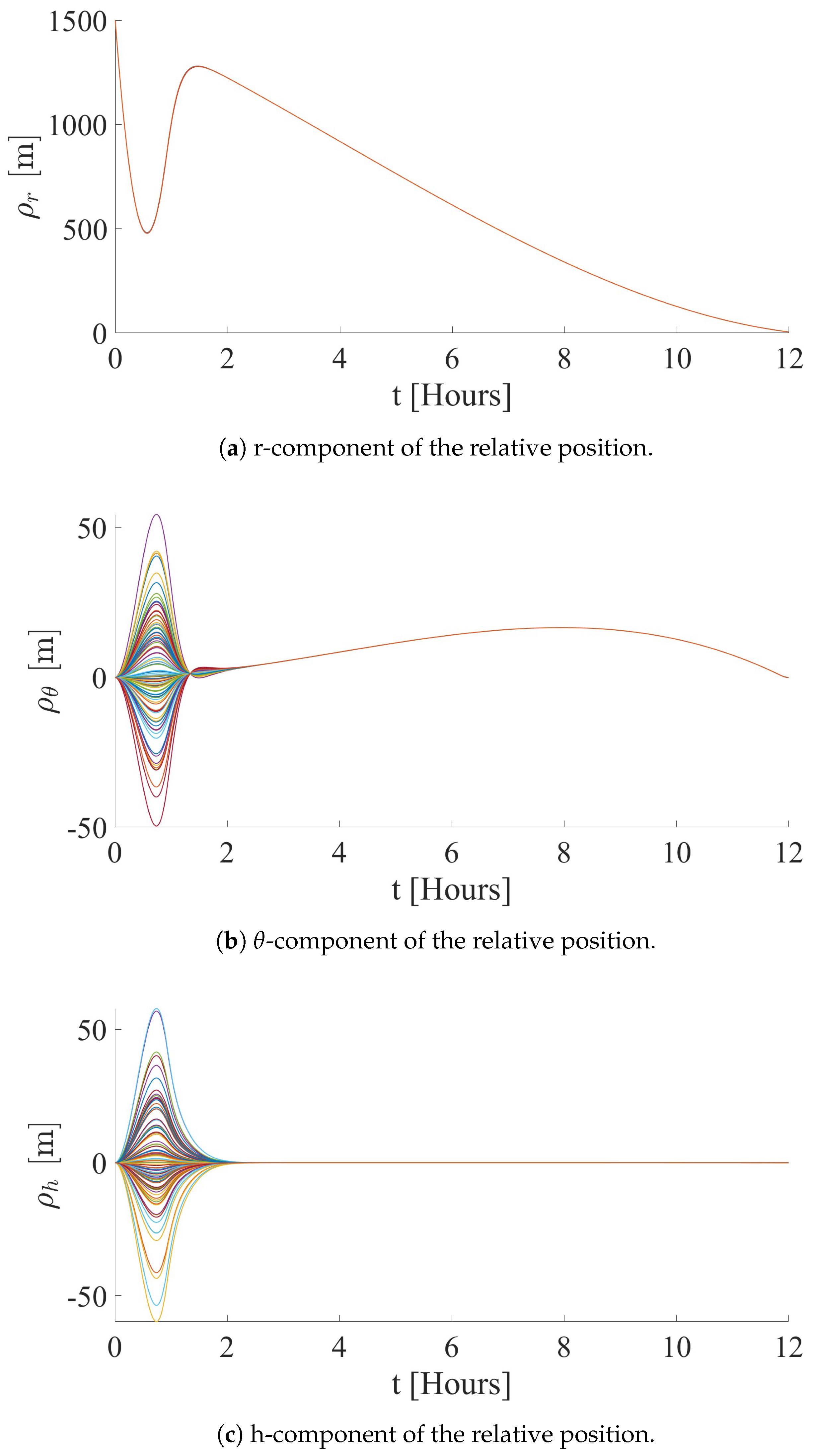
In order to prove its efficiency, the nonlinear hybrid predictive control is tested in several scenarios. Three cases are considered for tests in nominal conditions, where it is assumed that the control $\underline{u}$ provided by Equation (17) is applied. Each study presents a performance comparison between the constant-gain feedback linearization approach and hybrid predictive control. In all simulations, the starting epoch of the maneuver is set to 23 May 2025 at 10:00 UTC, while the final epoch corresponds to 23 May 2025 at 22:00 UTC. The final epoch coincides with a periselenium passage. This choice represents a sort of worst-case scenario, because the target has maximum velocity, and rendezvous is more challenging as a result. A predictive integration is performed every 2 min, through the forward propagation of the relative orbit dynamics by 30 min, in order to meet the criterion established in Section 5. However, in Section 6.3, the prediction rate is increased, and forward propagations are performed every 30 s, because relative orbit dynamics is faster. In all cases, the components of all vector quantities are expressed in the LVLH frame. All simulations are performed in a PC with i7-6700HQ processor and 32 GB of RAM.

6.1. Initial Radial Position ${\overrightarrow{\rho }}_0$ and Velocity ${\dot{\overrightarrow{\rho }}}_0$

Consider radial approaching as the initial conditions for rendezvous, with

$${\underline{\rho }}_0=\left(\begin{array}{c}1.5\\ 0\\ 0\end{array}\right)\mathrm{km},{\underline{\dot{\rho }}}_0=-\left(\begin{array}{c}1\\ 0\\ 0\end{array}\right)\mathrm{m}/\mathrm{s}$$

(26)

The control scheme and final desired state are described in Section 4. The resulting time evolution of the components of relative position and velocity is reported in Figure 4 and Figure 5, respectively. Thanks to the critical damping condition, the components of $\overrightarrow{\rho }$ have a smooth convergence toward the desired relative position, without overshooting. Using constant-gain feedback linearization, ${\rho }_r$ reaches ${\rho }_r=0$ in the first part of the maneuver. When this condition occurs, ${\rho }_{\theta }$ and ${\rho }_h$ are both below the Gateway radius, set to 5 m. Thus, this situation means that an impact with Gateway occurs. In contrast, nonlinear hybrid predictive control successfully drives the chaser state toward the desired final state. In fact, given a certain initial relative state, constant-gain feedback linearization requires much longer convergence time than the hybrid predictive control. This is due to the fact that feedback linearization uses the maximum available thrust only at the very beginning of the maneuver, as appears in Figure 6, where the norm of the thrust acceleration is illustrated. Looking at the thrust acceleration magnitude, a sudden drop at the end of the saturation time is evident. If the components of the thrust acceleration in Figure 7 are also taken into consideration, it can be noticed that this drop in thrust acceleration magnitude coincides with a change in the sign of $u_r$, which is the main component. This sign change corresponds to thrust direction reversal. Although the transition is rather steep, it is not instantaneous.

The trajectories followed by the chaser using both control algorithms are reported in Figure 8 and Figure 9. Due to the specific initial conditions, the motion is near monodimensional along $\widehat{r}$, with only a small component along $\widehat{\theta }$. This is in agreement with the modest value of $u_{\theta }$ that appears in Figure 7. The fact that the chaser does not only move along $\widehat{r}$ is caused by the introduction of a final drift phase. The final part of the trajectory obtained using nonlinear hybrid predictive control is depicted in Figure 10, where the drifting portion is highlighted. The final errors on relative position and velocity at the end of the rendezvous, i.e., at the end of the drifting phase, are reported in

Table 1. Desired terminal values and final errors on the relative state, using nonlinear hybrid predictive control.

	Desired Final Value	Final Error
${\rho }_r\left[\mathrm{m}\right]$	5	1.421 $\times {10}^{-6}$
${\rho }_{\theta }\left[\mathrm{m}\right]$	0	$-3.491\times {10}^{-7}$
${\rho }_h\left[\mathrm{m}\right]$	0	$-8.236\times {10}^{-11}$
${\dot{\rho }}_r\left[{\displaystyle \frac{\mathrm{cm}}{\mathrm{s}}}\right]$	−1	$3.665\times {10}^{-7}$
${\dot{\rho }}_{\theta }\left[{\displaystyle \frac{\mathrm{cm}}{\mathrm{s}}}\right]$	0	$1.345\times {10}^{-7}$
${\dot{\rho }}_h\left[{\displaystyle \frac{\mathrm{cm}}{\mathrm{s}}}\right]$	0	$-2.679\times {10}^{-11}$

. Only the results regarding the nonlinear hybrid predictive control are reported. It is evident that the final desired relative state is achieved with high accuracy.

6.2. Initial Radial Position ${\overrightarrow{\rho }}_0$ and Transversal Velocity ${\dot{\overrightarrow{\rho }}}_0$

Consider the following initial conditions for rendezvous

$${\underline{\rho }}_0=\left(\begin{array}{c}1.5\\ 0\\ 0\end{array}\right)\mathrm{km},{\underline{\dot{\rho }}}_0=\left(\begin{array}{c}0\\ 1\\ 1\end{array}\right)\mathrm{m}/\mathrm{s}$$

(27)

In this scenario, ${\dot{\overrightarrow{\rho }}}_0$ has zero components along $\widehat{r}$, therefore the chaser is not approaching Gateway at the beginning. Indeed, the initial relative velocity is orthogonal to the initial relative position. Therefore, orbit control needs to steer the velocity in order to have a negative component along $\widehat{r}$, while compensating the velocity components along $\widehat{\theta }$ and $\widehat{h}$. The resulting relative position and velocity components are reported in Figure 11 and Figure 12, respectively.

Also, in this case, nonlinear hybrid predictive control shows faster convergence toward the desired relative state with respect to constant-gain feedback linearization. The nonlinear hybrid predictive control succeeds in compensating the components of relative velocity along $\widehat{\theta }$ and $\widehat{h}$, and their effect on the respective components of relative position. At the same time, this control yields a modest r-component of relative velocity (of order of a few cm/s), which allows for the reaching of the desired final relative state in 12 h. On the contrary, constant-gain feedback linearization is not able to drive the system in a proper way in the required time interval. This is evident in Figure 13, where the chaser trajectories using both control algorithms are compared.

Since only the nonlinear hybrid predictive control proved to be effective in the case at hand, the following part of the analysis regards only this. The magnitude and components of the thrust acceleration are depicted in Figure 14 and Figure 15. Final errors on the relative state are shown in

Table 2. Desired terminal values and final errors on the relative state, using nonlinear hybrid predictive control.

	Desired Final Value	Final Error
${\rho }_r\left[\mathrm{m}\right]$	5	$1.416\times {10}^{-6}$
${\rho }_{\theta }\left[\mathrm{m}\right]$	0	$-3.499\times {10}^{-7}$
${\rho }_h\left[\mathrm{m}\right]$	0	$-8.237\times {10}^{-11}$
${\dot{\rho }}_r\left[{\displaystyle \frac{\mathrm{c}\mathrm{m}}{\mathrm{s}}}\right]$	−1	$3.655\times {10}^{-7}$
${\dot{\rho }}_{\theta }\left[{\displaystyle \frac{\mathrm{c}\mathrm{m}}{\mathrm{s}}}\right]$	0	$1.346\times {10}^{-7}$
${\dot{\rho }}_h\left[{\displaystyle \frac{\mathrm{c}\mathrm{m}}{\mathrm{s}}}\right]$	0	$-2.679\times {10}^{-11}$

.

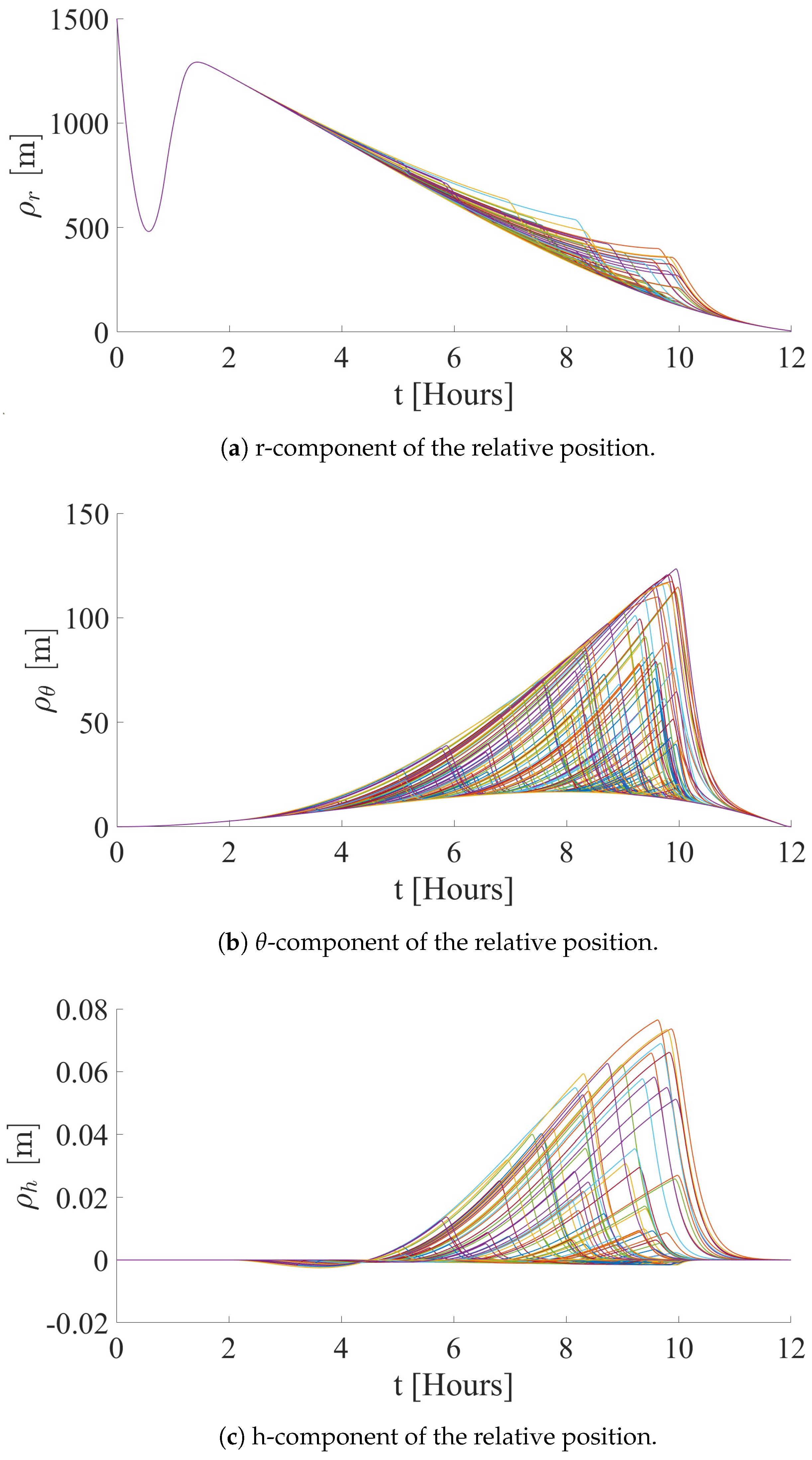
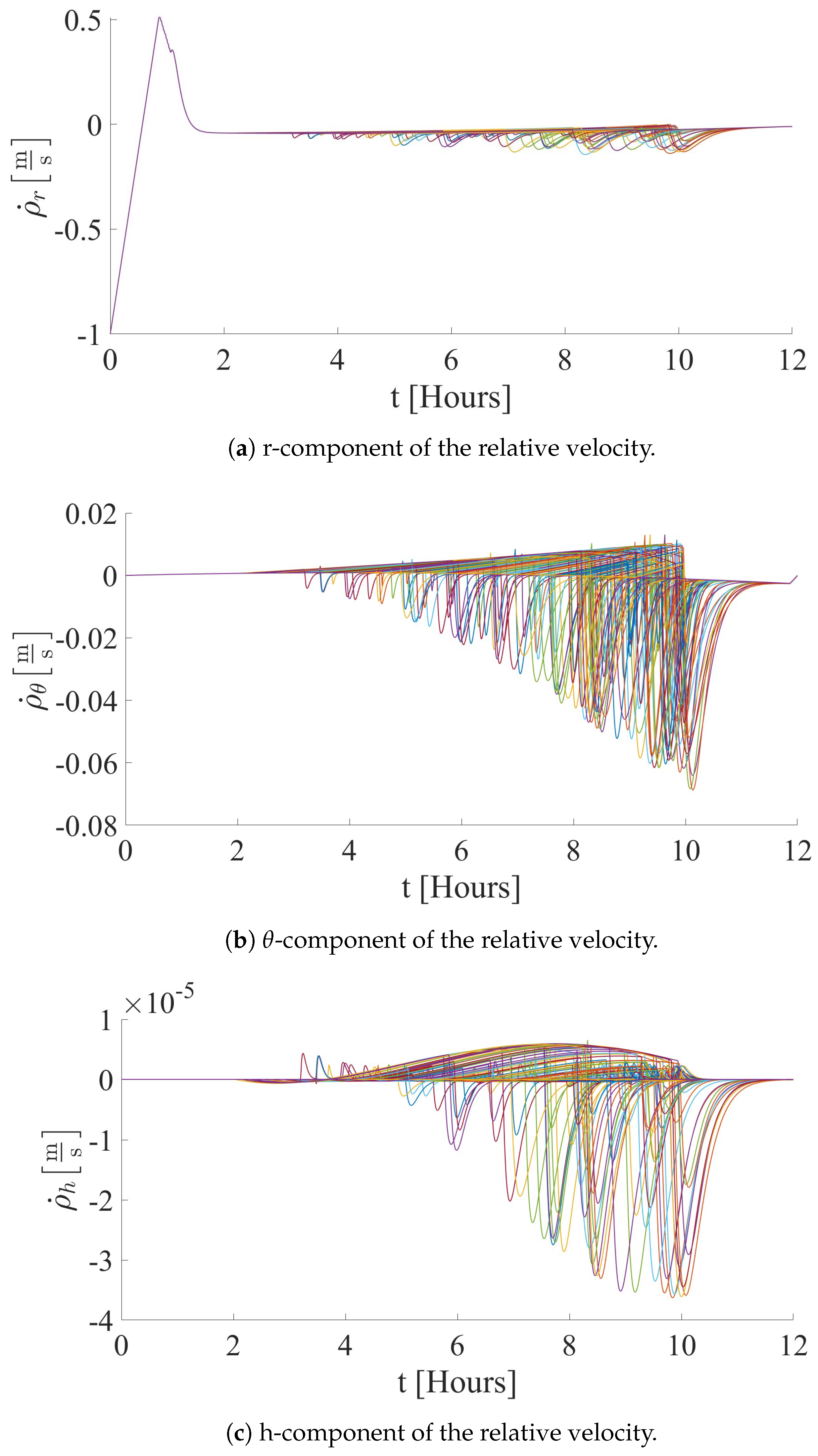
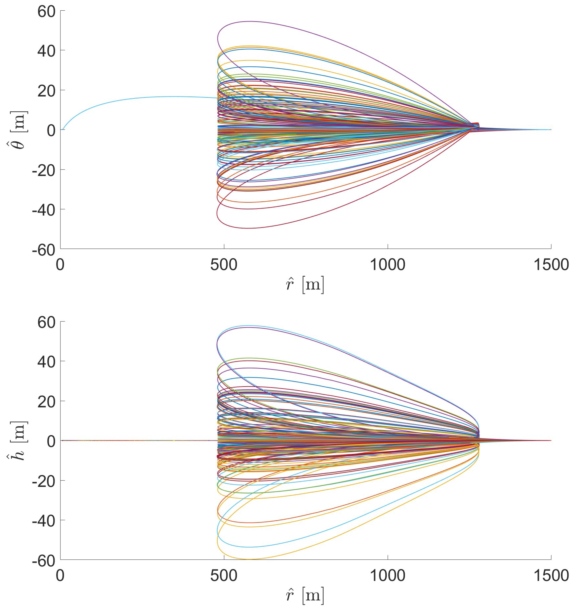
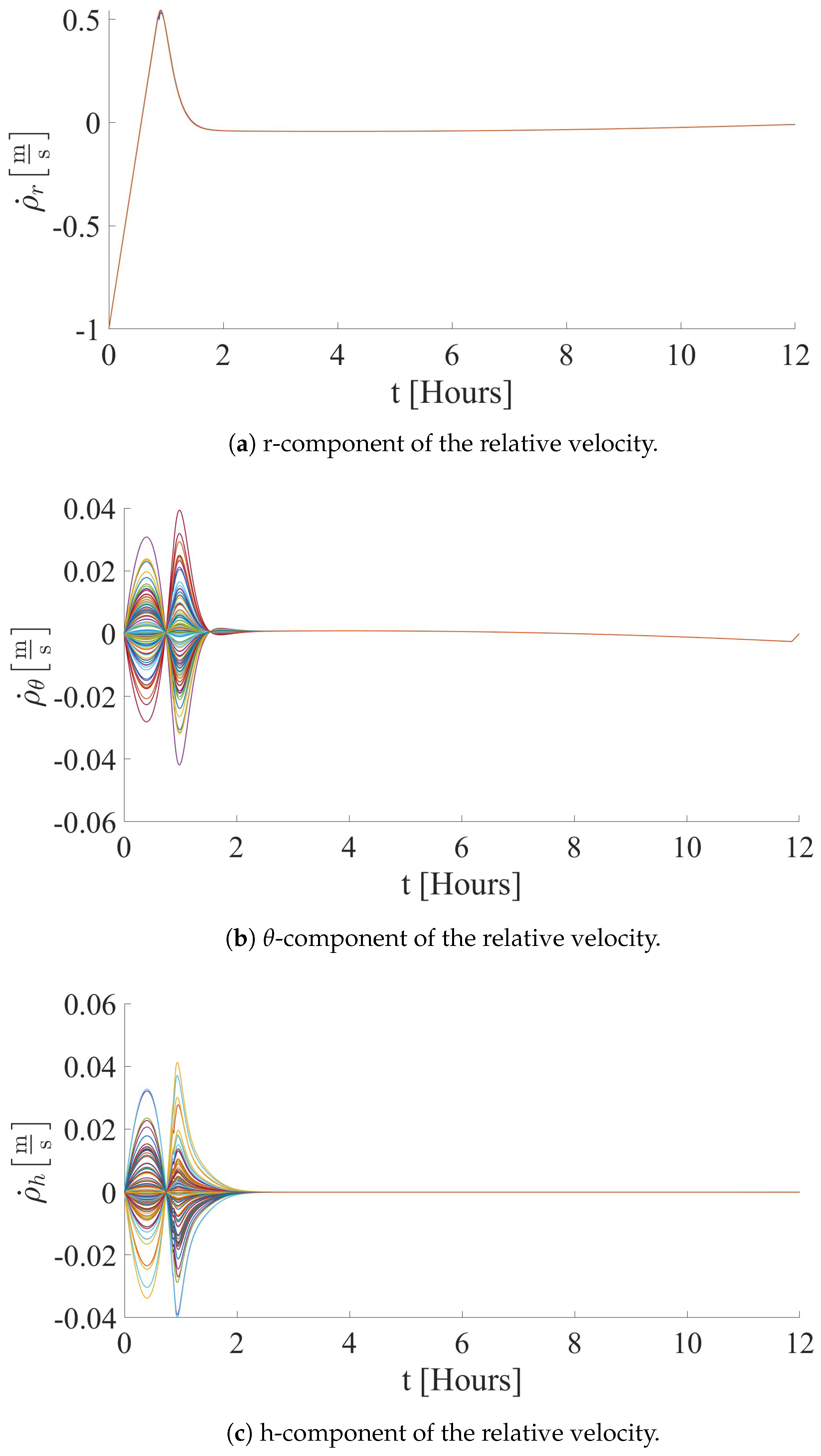
6.3. Relative Velocity Sphere

The time evolution of the relative state strongly depends on the initial relative velocity. In order to evaluate the performance of the control laws previously presented for different initial relative velocities, the following study is proposed. The initial relative position is chosen as

$${\underline{\rho }}_0=\left(\begin{array}{c}1.5\\ 0\\ 0\end{array}\right)\mathrm{km}$$

(28)

The magnitude of the initial relative velocity is set to a certain value. Then, 110 different directions in the LVLH-frame are considered. Each direction is associated with a point on a unit sphere. Overall, 110 points are selected: two of them coincide with the poles, whereas the remaining points are the intersections of nine equally-spaced parallels and 12 meridians. For each velocity direction, a simulation is performed. The outcomes are divided in three different classes:

• impact, when the relative distance reaches a value lower than 5 m;
• unsuccessful rendezvous, when at least one of the following situation occurs:
  • $u>u_{max}$ at any time;
  • the error on the norm of the final relative position or velocity is higher than $1\%$ of the desired value. For the desired final relative state, this implies a tolerance of 5 cm and 0.1 mm/s, respectively;
• successful rendezvous, when none of the previous cases occur.

In order to make the following figures clearer, a reference sphere with a radius equal to the magnitude of the relative velocity is depicted. The results corresponding to constant-gain feedback linearization are collected in Figure 16 and Figure 17. If ${\dot{\rho }}_0=$ 1 m/s, then negative radial relative velocity yields an impact. This is in agreement with the example shown in Section 6.1. However, other directions with negative radial components lead to successful rendezvous. Instead, the initial relative velocity directions with zero or positive radial velocity components are not properly tackled by the constant-gain feedback linearization. In this case, a large error on the final position (of an order of 1 m) is found. This is due to the ineffective use of the available thrust yielded by the use of constant gains, and this circumstance does not allow for the reaching of the final position in the desired time interval. Moreover, if ${\dot{\rho }}_0=$ 1.5 m/s, then no direction exists for the initial relative velocity, such that feedback linearization leads to a successful rendezvous.

If nonlinear hybrid predictive control is used, then successful rendezvous maneuvers are obtained until ${\dot{\rho }}_0$ = 3 m/s, as shown in Figure 18. However, increasing the magnitude of initial relative velocity to 5 m/s, directions with a sufficiently high positive radial direction lead to unsuccessful rendezvous. This situation is depicted in Figure 19. Also, in this case, the reason for the failure depends on the final relative position, which shows a maximum error of 14 cm on the radial component. Because 5 m/s is already a rather big initial relative velocity, the velocity sphere was not expanded further in this study.

7. Rendezvous in Nonnominal Conditions

The control law provides the desired thrust acceleration $\underline{u}$ at any time during rendezvous. However, the applied thrust acceleration is in general different from the commanded one, because of actuation errors. In order to evaluate the effects of these nonnominal conditions, two scenarios are considered:

• temporary propulsion unavailability;
• thrust pointing errors.

Since the hybrid predictive control proved to be better performing than constant-gain feedback linearization, in the following only the former control law is employed. The total time for rendezvous is set to 12 h: the maneuver begins on 23 May 2025 at 10:00 UTC and ends on 23 May 2025 at 22:00 UTC. The starting epoch coincides with a periselenium passage. The components of all vector quantities are expressed in the LVLH-frame. All simulations are carried out with the same initial relative state,

$${\underline{\rho }}_0=\left(\begin{array}{c}1.5\\ 0\\ 0\end{array}\right)\mathrm{km},{\underline{\dot{\rho }}}_0=-\left(\begin{array}{c}1\\ 0\\ 0\end{array}\right)\mathrm{m}/\mathrm{s}$$

(29)

Given the magnitude of initial relative position and velocity, these initial conditions represent the most challenging situation, as they require an important braking action in order to avoid collision with the target.

7.1. Temporary Propulsion Unavailability

During the rendezvous maneuver, the propulsion system may be turned off for several reasons:

• temporary malfunction;
• temporary reduction of electric power due to solar eclipse or power supply issues implying thrust unavailability;
• nonnominal attitude that is inconsistent with the desired thrust pointing direction, e.g., due to the requirement of different pointing of the antennas.

For the purpose of evaluating the effects of this occurrence, both the initial time and the duration of thrust unavailability are treated as uniformly distributed random variables. In particular, the occurrence time of the thrust unavailability, $t_{\ast }$, varies between the second and the tenth hour of the maneuver. This means that the first saturation period and the final phase are assumed to be unaffected by thrust unavailability. The duration, $\Delta t_{failure}$, is assumed to vary in the interval between one minute and $\Delta t_{max}$, where $\Delta t_{max}$ is the maximum possible duration of thrust unavailability. When propulsion is ignited again, Equation (25) is solved in order to find the highest $k_p$ that can be employed without exceeding $u_{max}$. Then, constant-gain feedback linearization is applied along the second thrusted phase.

A total number of 200 Monte Carlo (MC) simulations is run. A prediction rate equal to 30 s is employed in all simulated scenarios, i.e., the relative state is forward propagated in time for 30 min, every 30 s. The result of each rendezvous maneuver is categorized according to the same criterion stated in Section 6.3. The outcome is reported in Figure 20. The peculiar choice for the random variables creates a correlation between $t_{\ast }$ and $\Delta t_{failure}$, as apparent in Figure 20. In all cases, the control architecture compensates propulsion unavailability and completes a successful rendezvous (cf. Figure 21). Figure 22 and Figure 23 portray the components of the relative positions and velocities, respectively. During propulsion unavailability, the spacecraft follows natural drift. In general, the components of the relative state tend to diverge from the desired value in this period. However, it can be noticed that in all simulations successful recovery from this drift occurs, and convergence toward the final desired state is obtained. The main component of both position and velocity is along $\widehat{r}$, with a smaller component along $\widehat{\theta }$ and a negligible component along $\widehat{h}$. Therefore, the trajectories develop in the ($\widehat{r},\widehat{\theta }$)-plane, as shown in Figure 21. These results can also be regarded and interpreted in light of the simulation presented in Section 6.1. The mean error $\mu$ refers to the difference between the desired final value and the value obtained at the end of rendezvous, and is evaluated for each component of the relative state. Moreover, the corresponding standard deviation $\sigma$ is evaluated.

Table 3. Mean error and standard deviation for each component of the relative state. Desired final values are reported as a reference.

	Desired Final Value	$\mathit{\mu }$	$\mathit{\sigma }$
${\rho }_r\left[\mathrm{m}\right]$	5	$1.420\times {10}^{-3}$	$7.364\times {10}^{-3}$
${\rho }_{\theta }\left[\mathrm{m}\right]$	0	$7.552\times {10}^{-4}$	$4.701\times {10}^{-3}$
${\rho }_h\left[\mathrm{m}\right]$	0	$3.866\times {10}^{-7}$	$2.315\times {10}^{-6}$
${\dot{\rho }}_r\left[{\displaystyle \frac{\mathrm{cm}}{\mathrm{s}}}\right]$	−1	$-3.455\times {10}^{-4}$	$2.276\times {10}^{-3}$
${\dot{\rho }}_{\theta }\left[{\displaystyle \frac{\mathrm{cm}}{\mathrm{s}}}\right]$	0	$1.167\times {10}^{-4}$	$4.912\times {10}^{-4}$
${\dot{\rho }}_h\left[{\displaystyle \frac{\mathrm{cm}}{\mathrm{s}}}\right]$	0	$-1.287\times {10}^{-7}$	$7.144\times {10}^{-7}$

summarizes the overall results of the MC simulations.

7.2. Thrust Pointing Errors

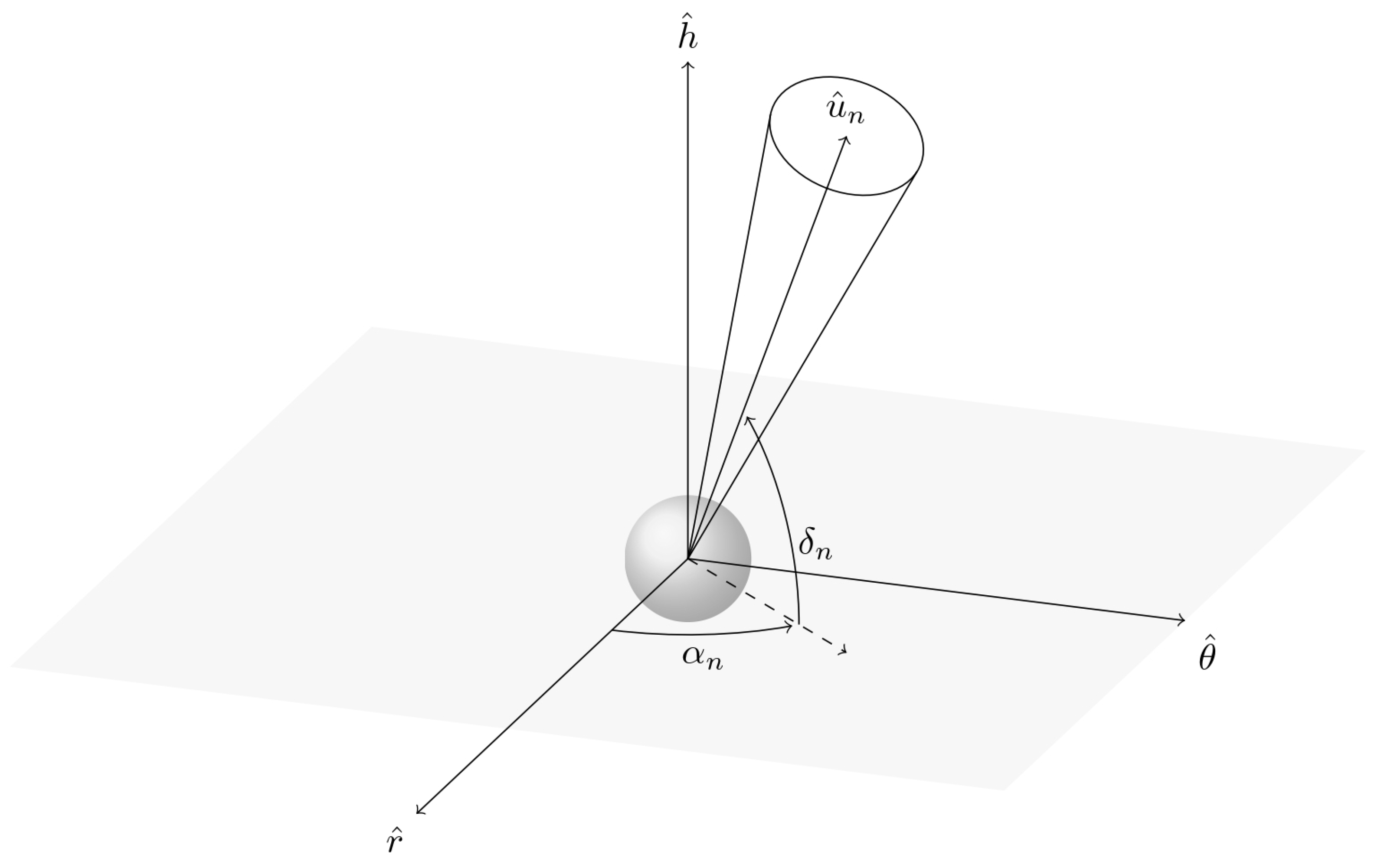
Consider the nominal commanded thrust, ${\overrightarrow{u}}_n$. In the LVLH-frame, the direction of ${\overrightarrow{u}}_n$ is identified by two angles, i.e., ${\delta }_n$ and ${\alpha }_n$ (cf. Figure 24),

$$\begin{array}{cc}\hfill u_{n,r}& =u_{n}cos{\delta }_{n}cos{\alpha }_n\hfill \\ \hfill u_{n,\theta }& =u_{n}cos{\delta }_{n}sin{\alpha }_n\hfill \\ \hfill u_{n,h}& =u_{n}sin{\delta }_n\hfill \end{array}$$

(30)

In this study, a pointing error is assumed to occur, and the actual thrust direction $\widehat{u}$ lies on the cone depicted in Figure 24. The displaced direction changes in each MC simulation, and is associated with two random angles illustrated in Figure 25:

• $\beta$, defined as the angle from $\widehat{i}$ and the projection of $\widehat{u}$ onto the ($\widehat{i},\widehat{j}$)-plane; it is generated as a uniform random variable ranging from 0 to $2\pi$;
• $\gamma$, defined as the angle between ${\widehat{u}}_n$ and $\widehat{u}$; it is generated according to a normal distribution, characterized by mean value $\mu =0^{\circ }$ and standard deviation $\sigma =2^{\circ }$. The distribution is truncated to $\pm 3\sigma$.

In Figure 25 unit vectors ($\widehat{i}$, $\widehat{j}$,) are defined as

$$\widehat{i}={\displaystyle \frac{{\widehat{u}}_n\times \widehat{h}}{|{\widehat{u}}_n\times \widehat{h}|}}\mathrm{and}\widehat{j}={\widehat{u}}_n\times \widehat{i}$$

(31)

After several steps, omitted for the sake of brevity, the displaced thrust direction in the LVLH-frame is given by

$$\begin{array}{cc}\hfill u_r& =u_n(sin\gamma cos\beta sin{\alpha }_n+sin\gamma sin\beta cos{\alpha }_{n}sin{\delta }_n+cos\gamma cos{\delta }_{n}cos{\alpha }_n)\hfill \\ \hfill u_{\theta }& =u_n(-sin\gamma cos\beta cos{\alpha }_n+sin\gamma sin\beta sin{\alpha }_{n}sin{\delta }_n+cos\gamma cos{\delta }_{n}sin{\alpha }_n)\hfill \\ \hfill u_h& =u_n(-sin\gamma sin\beta cos{\delta }_n+cos\gamma sin{\delta }_n)\hfill \end{array}$$

(32)

Figure 24. Pointing error cone around the nominal thrust direction ${\widehat{u}}_n$ in the LVLH-frame.

Figure 24. Pointing error cone around the nominal thrust direction ${\widehat{u}}_n$ in the LVLH-frame.

Figure 25. Representation of thrust misalignment.

Figure 25. Representation of thrust misalignment.

At the beginning of each simulation, $\beta$ and $\gamma$ are generated according to their respective random distribution, and a constant pointing error of $\widehat{u}$ relative to ${\widehat{u}}_n$ affects each MC simulation. A prediction rate equal to 2 min is employed in all simulated scenarios, i.e., the relative state is forward propagated in time for 30 min, every 2 min. The outcome of each simulation is evaluated according to the criterion presented in Section 6.3. A total of 200 MC simulations are run, and the related final results are illustrated in Figure 26 through Figure 27. All simulations yielded a positive outcome. Thus, the hybrid predictive nonlinear control law proved to be able to drive the spacecraft in a proper way, with a constant pointing error as well. As a matter of fact, this control law depends on the error between the desired state and actual state, and on its time derivatives. Therefore, at a certain time, a pointing error produces a greater error at the subsequent time step, but a higher error creates a stronger response by the feedback control law, which reduces the error.

In Figure 28 and Figure 29, the LVLH components of relative position and velocity are reported, respectively. The trajectories obtained in the MC campaign are represented in Figure 27. For the sake of clarity, the results of only 100 simulations are shown in these plots. The time histories of the relative state components along $\widehat{\theta }$ and $\widehat{h}$ are roughly symmetric, unlike the remaining radial component. This is due to the fact that the latter is subject to most of the control effort, because of the specific initial conditions. This is apparent in Figure 30, in which the component $u_r$ is larger than the other ones; this illustrative example corresponds to $\gamma =5.6^{\circ }$ and $\beta =32.4^{\circ }$. The collection of 100 relative trajectories, portrayed in Figure 27, reflect the symmetry noted for the relative position components. The mean final error $\mu$ and the corresponding standard deviation $\sigma$ are computed for each LVLH component of the relative state, employing the data coming from the MC campaign. These results are collected in

Table 4. Mean error and standard deviation for each component of the relative state. Desired final values are reported as a reference.

	Desired Final Value	$\mathit{\mu }$	$\mathit{\sigma }$
${\rho }_r\left[\mathrm{m}\right]$	5	$8.596\times {10}^{-3}$	$1.467\times {10}^{-2}$
${\rho }_{\theta }\left[\mathrm{m}\right]$	0	$-6.453\times {10}^{-4}$	$6.410\times {10}^{-3}$
${\rho }_h\left[\mathrm{m}\right]$	0	$-1.080\times {10}^{-5}$	$2.432\times {10}^{-2}$
${\dot{\rho }}_r\left[{\displaystyle \frac{\mathrm{cm}}{\mathrm{s}}}\right]$	−1	$-1.067\times {10}^{-4}$	$9.519\times {10}^{-4}$
${\dot{\rho }}_{\theta }\left[{\displaystyle \frac{\mathrm{cm}}{\mathrm{s}}}\right]$	0	$-5.239\times {10}^{-4}$	$1.009\times {10}^{-3}$
${\dot{\rho }}_h\left[{\displaystyle \frac{\mathrm{cm}}{\mathrm{s}}}\right]$	0	$-2.423\times {10}^{-7}$	$4.961\times {10}^{-4}$

.

8. Conclusions

This research addresses relative orbit dynamics and control, applied to rendezvous maneuvers in cislunar space. An advantageous reformulation of the BG approach to relative orbit motion is introduced, and allows for the obtaining of a description that does not assume any linearizing approximation. Moreover, this new dynamical framework can include all the relevant orbit perturbations, on both spacecraft, without introducing any simplifying assumption on the target orbit, which instead must be Keplerian in the classical, well-established formulation of the BG equations. A new nonlinear hybrid predictive control is also introduced that leverages gain adaptation. This new guidance strategy assumes time-varying gains in the first phase. They are selected by enforcing saturation of the thrust magnitude. In the second phase, the classical feedback linearization scheme is applied, while avoiding the violation of the maximum allowed thrust magnitude. This goal is achieved through predictive propagations, which definitely determine the midway time to step from phase 1 to phase 2. An extensive parametric analysis is presented in terms of relative velocity magnitude and direction, and the novel guidance approach at hand is shown to outperfom pure feedback linearization, with regard to both the rendezvous success rate and the accuracy of the actual final relative state with respect to the desired one. The rendezvous strategy with Gateway includes a final, unpowered drift phase, for safety reasons, and also to accommodate possible attitude maneuvers. Furthermore, a Monte Carlo analysis points out that the new orbit control approach at hand is very effective, even when the chaser spacecraft experiences stochastic thrust unavailability or in the presence of relatively large thrust pointing errors. Because the simulation runtime is by far shorter than the total duration of rendezvous, hybrid predictive control can be deemed to be an effective real-time technique in orbit rendezvous maneuvers toward Gateway.

References

1. NASA. Artemis Plan. 2020. Available online: https://www.nasa.gov/wp-content/uploads/2020/12/artemis_plan-20200921.pdf (accessed on 12 January 2024).
2. NASA. What Is CAPSTONE? Available online: https://www.nasa.gov/smallspacecraft/capstone/ (accessed on 12 January 2024).
3. Howell, K.C.; Kakoi, M. Transfers between the Earth–Moon and Sun–Earth systems using manifolds and transit orbits. Acta Astronaut. 2006, 59, 367–380. [Google Scholar] [CrossRef]
4. Alessi, E.M.; Gomez, G.; Masdemont, J.J. Two-manoeuvres transfers between LEOs and Lissajous orbits in the Earth–Moon system. Adv. Space Res. 2010, 45, 1276–1291. [Google Scholar] [CrossRef]
5. Pontani, M.; Teofilatto, P. Polyhedral representation of invariant manifolds applied to orbit transfers in the Earth–Moon system. Acta Astronaut. 2016, 119, 218–232. [Google Scholar] [CrossRef]
6. Singh, S.K.; Anderson, B.D.; Taheri, E.; Junkins, J.L. Low-thrust transfers to southern L 2 near-rectilinear halo orbits facilitated by invariant manifolds. J. Optim. Theory Appl. 2021, 191, 517–544. [Google Scholar] [CrossRef]
7. Parrish, N.L.; Parker, J.S.; Hughes, S.P.; Heiligers, J. Low-thrust transfers from distant retrograde orbits to L2 halo orbits in the Earth-Moon system. In Proceedings of the International Conference on Astrodynamics Tools and Techniques 2016, Darmstadt, Germany, 14–17 March 2016. [Google Scholar]
8. Pino, B.P.; Howell, K.C.; Folta, D. An energy-informed adaptive algorithm for low-thrust spacecraft cislunar trajectory design. In Proceedings of the AAS/AIAA Astrodynamics Specialist Conference, 2020, South Lake Tahoe, CA, USA, 9–12 August 2020. [Google Scholar]
9. Pritchett, R.E. Strategies for Low-Thrust Transfer Design Based on Direct Collocation Techniques. Ph.D. Thesis, Purdue University, West Lafayette, IN, USA, 2020. [Google Scholar]
10. Das-Stuart, A.; Howell, K.C.; Folta, D.C. Rapid trajectory design in complex environments enabled by reinforcement learning and graph search strategies. Acta Astronaut. 2020, 171, 172–195. [Google Scholar] [CrossRef]
11. McCarty, S.L.; Burke, L.M.; McGuire, M. Parallel monotonic basin hopping for low thrust trajectory optimization. In Proceedings of the 2018 Space Flight Mechanics Meeting, Kissimmee, FL, USA, 8–12 January 2018; p. 1452. [Google Scholar]
12. Vutukuri, S. Spacecraft Trajectory Design Techniques Using Resonant Orbits. Master’s Thesis, Purdue University, West Lafayette, IN, USA, 2018. [Google Scholar]
13. Zimovan-Spreen, E.M.; Howell, K.C. Dynamical structures nearby NRHOS with applications in cislunar space. In Proceedings of the AAS/AIAA Astrodynamics Specialist Conference 2019, Portland, ME, USA, 10–15 August 2019; p. 18. [Google Scholar]
14. Whitley, R.; Martinez, R. Options for staging orbits in cislunar space. In Proceedings of the 2016 IEEE Aerospace Conference, Big Sky, MT, USA, 5–12 March 2016; pp. 1–9. [Google Scholar]
15. Rozek, M.; Ogawa, H.; Ueda, S.; Ikenaga, T. Multi-objective optimisation of NRHO-LLO orbit transfer via surrogate-assisted evolutionary algorithms. In Proceedings of the 27th International Symposium on Space Flight Dynamics, Melbourne, Australia, 24–28 February 2019. [Google Scholar]
16. Lu, L.; Li, H.; Zhou, W.; Liu, J. Design and analysis of a direct transfer trajectory from a near rectilinear halo orbit to a low lunar orbit. Adv. Space Res. 2021, 67, 1143–1154. [Google Scholar] [CrossRef]
17. Bucchioni, G.; Innocenti, M. Phasing maneuver analysis from a low lunar orbit to a near rectilinear halo orbit. Aerospace 2021, 8, 70. [Google Scholar] [CrossRef]
18. Giordano, C.; Topputo, F. Analysis, Design, and Optimization of Robust Trajectories in Cislunar Environment for Limited-Capability Spacecraft. J. Astronaut. Sci. 2023, 70, 53. [Google Scholar] [CrossRef]
19. Sanna, D.; Leonardi, E.M.; De Angelis, G.; Pontani, M. Optimal Impulsive Orbit Transfers from Gateway to Low Lunar Orbit. Aerospace 2024, 11, 460. [Google Scholar] [CrossRef]
20. Pozzi, C.; Pontani, M.; Beolchi, A.; Fantino, E. Optimization, guidance, and control of low-thrust transfers from the Lunar Gateway to low lunar orbit. Acta Astronaut. 2024, 222, 39–51. [Google Scholar] [CrossRef]
21. Lee, D.E.; Whitley, R.J.; Acton, C. Sample Deep Space Gateway Orbit. 2018. Available online: https://naif.jpl.nasa.gov/pub/naif/misc/MORE_PROJECTS/DSG/ (accessed on 12 January 2024).
22. Zimovan-Spreen, E.M.; Davis, D.C.; Howell, K.C. Recovery Traejctories for Inadvertent Departures from an NRHO. In Proceedings of the AAS/AIAA Spaceflight Mechanics Meeting 2021, Virtual, 1–4 February 2021. number AAS 21-345. [Google Scholar]
23. Alvarado, K.I.; Singh, S.K. Exploration and Maintenance of Homeomorphic Orbit Revs in the Elliptic Restricted Three-Body Problem. Aerospace 2024, 11, 407. [Google Scholar] [CrossRef]
24. Pontani, M.; Conway, B.A. Optimal Finite-Thrust Rendezvous Trajectories Found via Particle Swarm Algorithm. J. Spacecr. Rocket. 2013, 50, 1222–1234. [Google Scholar] [CrossRef]
25. Bevilacqua, R.; Lovell, T.A. Analytical guidance for spacecraft relative motion under constant thrust using relative orbit elements. Acta Astronaut. 2014, 102, 47–61. [Google Scholar] [CrossRef]
26. Gurfil, P. Relative Motion between Elliptic Orbits: Generalized Boundedness Conditions and Optimal Formationkeeping. J. Guid. Control. Dyn. 2005, 28, 761–767. [Google Scholar] [CrossRef]
27. Lopez, I.; Mclnnes, C.R. Autonomous rendezvous using artificial potential function guidance. J. Guid. Control. Dyn. 1995, 18, 237–241. [Google Scholar] [CrossRef]
28. Kluever, C.A. Feedback Control for Spacecraft Rendezvous and Docking. J. Guid. Control. Dyn. 1999, 22, 609–611. [Google Scholar] [CrossRef]
29. Karlgaard, C.D. Robust Rendezvous Navigation in Elliptical Orbit. J. Guid. Control. Dyn. 2006, 29, 495–499. [Google Scholar] [CrossRef]
30. Santoro, R.; Pontani, M. Orbit acquisition, rendezvous, and docking with a noncooperative capsule in a Mars sample return mission. Acta Astronaut. 2023, 211, 950–962. [Google Scholar] [CrossRef]
31. Anand, N.; Kumar, S.R. Nonsingular Finite-Time Convergent Control for Spacecraft Rendezvous and Docking. In Proceedings of the 22nd IFAC World Congress, Yokohama, Japan, 9–14 July 2023; Volume 56, pp. 2007–2012. [Google Scholar] [CrossRef]
32. Capello, E.; Punta, E.; Dabbene, F.; Guglieri, G.; Tempo, R. Sliding-Mode Control Strategies for Rendezvous and Docking Maneuvers. J. Guid. Control. Dyn. 2017, 40, 1481–1487. [Google Scholar] [CrossRef]
33. Li, Q.; Yuan, J.; Wang, H. Sliding mode control for autonomous spacecraft rendezvous with collision avoidance. Acta Astronaut. 2018, 151, 743–751. [Google Scholar] [CrossRef]
34. Lee, D.E. White Paper: Gateway Destination Orbit Model: A Continuous 15 Year NRHO Reference Trajectory; Technical report; NASA: Washington, DC, USA, 2019.
35. Davis, D.; Bhatt, S.; Howell, K.; Jang, J.W.; Whitley, R.; Clark, F.; Guzzetti, D.; Zimovan, E.; Barton, G. Orbit maintenance and navigation of human spacecraft at cislunar near rectilinear halo orbits. In Proceedings of the AAS/AIAA Space Flight Mechanics Meeting 2017, San Antonio, TX, USA, 5–9 February 2017. [Google Scholar]
36. Davis, D.C.; Phillips, S.M.; Howell, K.C.; Vutukuri, S.; McCarthy, B.P. Stationkeeping and transfer trajectory design for spacecraft in cislunar space. In Proceedings of the AAS/AIAA Astrodynamics Specialist Conference 2017, Stevenson, WA, USA, 20–24 August 2017; Volume 8. [Google Scholar]
37. Li, S.; Lucey, P.G.; Milliken, R.E.; Hayne, P.O.; Fisher, E.; Williams, J.P.; Hurley, D.M.; Elphic, R.C. Direct evidence of surface exposed water ice in the lunar polar regions. Proc. Natl. Acad. Sci. USA 2018, 115, 8907–8912. [Google Scholar] [CrossRef] [PubMed]
38. McGuire, M.L.; McCarty, S.L.; Burke, L.M. Power & Propulsion Element (PPE) Spacecraft Reference Trajectory Document; Glenn Research Center: Cleveland, OH, USA, 2018; Volume PPE-DOC-0079, pp. 4–5. [Google Scholar]
39. Kéchichian, J.A. Orbital Relative Motion and Terminal Rendezvous: Analytic and Numerical Methods for Spaceflight Guidance Applications; Springer International Publishing: Berlin/Heidelberg, Germany, 2021; pp. 1–17. [Google Scholar] [CrossRef]
40. Pontani, M. Advanced Spacecraft Dynamics, 1st ed.; Edizioni Efesto: Rome, Italy, 2023. [Google Scholar]
41. Varberg, D.; Purcell, E.; Rigdon, S. Calculus with Differential Equations, 9th ed.; Prentice Hall: Hoboken, NJ, USA, 2006. [Google Scholar]
Figure 1. Gateway trajectory in the Earth–Moon synodic reference frame, for ten periods.
Dynamics 04 00032 g001
Figure 2. Time history of the thrust acceleration magnitude, yielded through feedback linearization. Initial conditions: ρ ̲ = ( 1.5 , 0 , 0 ) T km, ρ ˙ ̲ = ( 1 , 0 , 0 ) T m/s.
Dynamics 04 00032 g002
Figure 3. Thrust acceleration profile for several saturation time intervals Δ t s a t . Initial conditions: ρ ̲ = ( 1.5 , 0 , 0 ) T km, ρ ˙ ̲ = ( 1 , 0 , 0 ) T m/s.
Dynamics 04 00032 g003
Figure 4. Components of the relative position using either constant–gain feedback linearization or nonlinear hybrid predictive control.
Dynamics 04 00032 g004
Figure 5. LVLH components of relative velocity using either constant–gain feedback linearization or nonlinear hybrid predictive control.
Dynamics 04 00032 g005aDynamics 04 00032 g005b
Figure 6. Thrust acceleration magnitude using either constant–gain feedback linearization or nonlinear hybrid predictive control. As a reference, the magnitude of the acceleration due to the natural relative motion f ̲ is reported.
Dynamics 04 00032 g006
Figure 7. LVLH components of the thrust acceleration required by the nonlinear hybrid predictive control.
Dynamics 04 00032 g007
Figure 8. Rendezvous trajectory followed by the chaser using both control algorithms. θ ^ axis is expanded for clarity.
Dynamics 04 00032 g008
Figure 9. Zoom on the region around Gateway. The red dashed circle represents the 5 m sphere of Gateway.
Dynamics 04 00032 g009
Figure 10. Final drift followed by the chaser, following thrusted arc with the use of nonlinear hybrid predictive control. Green and red dashed circles represent the two spheres centered at Gateway’s mass center center, with radii of 10 and 5 m, respectively.
Dynamics 04 00032 g010
Figure 11. LVLH components of relative position using either constant–gain feedback linearization or nonlinear hybrid predictive control.
Dynamics 04 00032 g011
Figure 12. LVLH components of relative velocity using either constant–gain feedback linearization or nonlinear hybrid predictive control.
Dynamics 04 00032 g012
Figure 13. Rendezvous trajectory using both control algorithms.
Dynamics 04 00032 g013
Figure 14. Thrust acceleration magnitude using either constant–gain feedback linearization or nonlinear hybrid predictive control. As a reference, the magnitude of the acceleration due to the natural relative motion f is reported.
Dynamics 04 00032 g014
Figure 15. LVLH components of the thrust acceleration required by the nonlinear hybrid predictive control.
Dynamics 04 00032 g015
Figure 16. Representation of the outcomes for different initial relative velocity directions, using constant–gain feedback linearization ( ρ ˙ 0 = 1 m/s).
Dynamics 04 00032 g016
Figure 17. Representation of the outcomes for different initial relative velocity directions, using constant–gain feedback linearization ( ρ ˙ 0 = 1.5 m/s).
Dynamics 04 00032 g017
Figure 18. Representation of the outcomes for different initial relative velocity directions, using hybrid predictive control linearization ( ρ ˙ 0 = 3 m/s).
Dynamics 04 00032 g018
Figure 19. Representation of the outcomes for different initial relative velocity directions, using hybrid predictive control linearization ( ρ ˙ 0 = 5 m/s).
Dynamics 04 00032 g019
Figure 20. Rendezvous outcomes for several initial times and durations of thrust unavailability.
Dynamics 04 00032 g020
Figure 21. Relative trajectories obtained in the Monte Carlo campaign.
Dynamics 04 00032 g021
Figure 22. Time histories of relative position obtained in the Monte Carlo campaign.
Dynamics 04 00032 g022
Figure 23. Time histories of relative velocity obtained in the Monte Carlo campaign.
Dynamics 04 00032 g023
Figure 26. Rendezvous outcome according to the respective pointing error. Dashed concentric circumferences indicate, outward from the center, γ = 1 σ , 2 σ , 3 σ .
Dynamics 04 00032 g026
Figure 27. Relative trajectories obtained in the Monte Carlo campaign.
Dynamics 04 00032 g027
Figure 28. Time histories of relative velocity obtained in the Monte Carlo campaign.
Dynamics 04 00032 g028
Figure 29. Time histories of relative velocity obtained in the Monte Carlo campaign.
Dynamics 04 00032 g029
Figure 30. Thrust acceleration components (illustrative example with γ = 5 . 6 and β = 32 . 4 ).
Dynamics 04 00032 g030