
Lid-Driven Cavity Flow Containing a Nanofluid


1
Department of Science and Technology, University of Hafr Al Batin, Hafr Al Batin 31991, Saudi Arabia
2
Department of Mathematics, University of Manchester, Manchester M13 9PL, UK
*
Author to whom correspondence should be addressed.
Dynamics 2024, 4(3), 671-697; https://doi.org/10.3390/dynamics4030034
Submission received: 2 July 2024
/
Revised: 30 July 2024
/
Accepted: 7 August 2024
/
Published: 15 August 2024
Abstract
:In this paper, we consider the flow of a nanofluid in an enclosed lid-driven cavity using a single-phase model. Two cases are considered: one in which the top and bottom walls are kept at adiabatic conditions, and a second case in which the left- and right-side walls are kept in adiabatic conditions. The impact of different viscosity models on the mixed convection heat transfer is examined, and numerical methods are used to obtain solutions for the Navier–Stokes equations for various parameter ranges. Using our robust methods, we are able to obtain novel solutions for large Reynolds numbers and very small Richardson numbers. Using water as the base fluid and aluminium oxide nanoparticles, our results suggest that heat transfer enhancement occurs with increasing particle concentration and decreasing Richardson numbers. There are also significant differences depending on the viscosity model used in terms of the impact of reducing corner recirculation regions in the cavity.
1. Introduction
Many researchers have attempted to deal with issues that can alter the heat transfer performance of conventional fluids. These fluids include glycerol, water, thermal oils, ethylene glycol, and many more. To improve this performance, Choi [1] created a nanofluid containing nanoparticles smaller than 100 nm in conventional fluids. Numerous studies on the properties of nanofluids have concluded that nanofluids display higher thermal conductivity and heat transfer than base fluids [2,3,4]. Other research projects have focused on investigating the mechanisms of thermal conductivity of nanofluids and built simulation models to explain the phenomena. Conventional heat transfer fluids, such as water and ethylene glyco inside an enclosure, have limited heat transfer effectiveness as they have lower thermal conductivity compared with solids. Adding small solid particles (millimeter to micrometer-sized) is not effective as these particles settle with time and clog the flow channels, especially in miniaturized cooling systems, due to narrow flow channels. Using certain well-suspended nanofluids instead has shown greater stability with lower clogging rates and better heat transfer potential [5,6].
The phenomenon of mixed convection is widely employed in a variety of engineering processes, such as the operation of solar collectors, heat exchangers, drying technologies, home ventilation, high-performance building insulation, and lubrication technologies [7,8,9]. Mixed convection is more challenging computationally than other types of convection because of the interaction between buoyancy force, which is caused by temperature differences, and shear force, which is caused by wall movement.
Researchers have employed various numerical methods, such as the finite difference, finite element, and spectral methods, to simulate the lid-driven cavity problem. Lid-driven cavity flow is a typical benchmark problem for testing numerical techniques for the Navier–Stokes equations. In a square lid-driven cavity, laminar mixed convection flows of copper–water nanofluid were investigated numerically by [10] using the finite volume method. The Pak and Cho [11] and Brinkman [12] models were used in determining the thermal conductivity and effective dynamic viscosity of nanofluids, respectively. In these studies, particle volume fractions between 0 and 0.05, Reynolds numbers from 1 to 100, and Rayleigh numbers between and were considered. It was discovered that, at a fixed Reynolds number, the particle concentration impacts the flow characteristics and thermal behavior, especially at a larger Rayleigh number. Additionally, it is noted that when the Reynolds number increases, the impact of particle concentration reduces.
In a square cavity with laminar mixed convection fluid flow and heat transfer, ref. [13] examined the effects of different dynamic viscosity models with nanoparticles of different volume fractions. The enclosure’s left and right vertical walls and top wall were all kept at a constant temperature, and the bottom wall had a higher temperature than the other walls and moved from left to right. To evaluate the effective nanofluid dynamic viscosity, two distinct models, the Brinkman [12] and Maiga [14] models, were applied. Using the finite volume approach and the SIMPLER algorithm, the governing equations in primitive variable form were solved numerically. It was found that the magnitude of heat transfer enhancement was affected by the different viscosity models used.
Sheikhzadeh et al. [15] combined different thermal conductivity and viscosity formulas to investigate the properties of mixed convection heat transfer in a lid-driven cavity filled with nanofluids, which contained Al2O3 nanoparticles. The right and left walls were maintained at different fixed temperatures, whilst the top surface moved at a constant speed. The top and bottom walls remained insulated. The investigation was conducted using various solid volume fractions, Richardson numbers, and Grashof numbers up to . The findings of this research demonstrate that given a fixed solid volume fraction, the average Nusselt number varies depending on the thermal conductivity and viscosity models used. It was realized that the average Nusselt number was more susceptible to the viscosity and thermal conductivity formulas at small Richardson numbers. They used a control-volume-based finite volume technique and the SIMPLE algorithm.
Steady laminar mixed convection flow in square cavities, with a similar water-Al2O3 nanofluid in single and double lid-driven cavities, were modeled numerically by Chamkha and Abu-Nada [16]. The Pak and Cho and Brinkman formulas are the two viscosity formulas that were used to approximate the nanofluid viscosity in their research. They suggested that the existence of nanoparticles can significantly improve heat transfer by increasing the nanoparticle volume fractions at low and large Richardson numbers. The Pak and Cho model predicts that the existence of nanoparticles will result in a decrease in the average Nusselt number in the single-lid cavity model for small Richardson numbers. To numerically solve the system of equations, they employed a second-order finite-volume approach. Ghafouri et al. [17] examined how different thermal conductivity models affect the combined convection heat transfer in a square cavity. The nanofluid that was used in this study was water fluid with Al2O3 particles. The right and left walls were maintained at various constant temperatures, while the top and bottom walls were kept insulated, moving at a constant speed. To assess the impacts of numerous factors, including the size and volume fraction of the nanoparticles, the bulk temperature of the nanofluid, and Brownian motion, five distinct thermal conductivity models were applied. The streamfunction–vorticity equations were solved numerically using a second-order finite difference method. They also found that heat transfer is enhanced by increasing particle concentrations and decreasing the Richardson number.
In this paper, we investigate the steady Navier–Stokes equations for flow in a lid-driven cavity with two different dynamic viscosity formulas. The problem studied here is slightly different from the standard lid-driven cavity problem because of the coupling with the temperature field. Our aim is to investigate the role played by different viscosity models and the effect of a nanofluid in heat transfer enhancement. Another objective is to use more robust and accurate numerical approaches based on spectral methods. We aim to investigate parameter values where other researchers have encountered difficulties, particularly large Reynolds numbers and low Richardson numbers. We focus on obtaining results for a water-based Al2O3 nanofluid, but the techniques used here apply equally to other nanofluid combinations.
2. Mathematical Formulation
Consider two cases for the flow in a square lid-driven cavity with a width and a height of H. In the first case, which we denote as Case A, the top wall of the enclosure operates at an elevated temperature (), and the bottom wall of the enclosure remains at a lower constant temperature (). The top wall moves to the right with a constant speed . A schematic of the flow is shown in Figure 1. The right and left walls of the enclosure are maintained at adiabatic conditions. The nanofluid in the enclosed space is shown as a dilute solid–liquid fluid with uniform nanoparticles, such as Al2O3, scattered inside a base fluid, such as water.
For the second case, which we label as Case B, the left wall of the enclosure operates at an elevated temperature (), and the right wall of the enclosure remains at a lower constant temperature (). The top and bottom of the enclosure wall are maintained in adiabatic conditions. The top wall again moves to the right with constant speed . A schematic of the flow is shown in Figure 2.
The fundamental governing equations for the steady-state two-dimensional incompressible nanofluid flow are as follows. The vorticity (), stream function , and temperature () satisfy the following equations:
where is the density of the nanofluid, is the dynamic viscosity, is the thermal expansion coefficient, g is the acceleration due to gravity, and is the mixture thermal diffusivity.
The governing equations are nondimensionalized by introducing the following dimensionless variables:
The non-dimensional form of the equations are as follows:
The thermal expansion coefficient is
Dynamic viscosity and thermal conductivity are two major aspects of nanofluid transport. Numerous theoretical and experimental studies have been conducted, and numerous correlations have been established to estimate the dynamic viscosity and thermal conductivity of nanofluids.
The effective thermal conductivity ratio formula which we used and which is known as the Maxwell formula [18] is as follows:
where .
The dynamic viscosity in Brinkman’s formula [12] is given by the following:
and is frequently used in many studies. The other formula that we also used was found by fitting experimental data in [11] and is the Pak and Cho correlation given by the following:
Table 1 lists the thermophysical properties of the base fluid (water) and the nanoparticles Al2O3, which we used in this study, and these are as listed by Chamkha and Abu-Nada [16].
Finally to complete the description, we also require boundary conditions. We studied two cases, which we labeled as case A and case B.
For case A, we had no slip on and adiabatic conditions on the temperature given by
In addition, on the top wall, , representing the moving lid with a fixed temperature, we had the following:
On the bottom wall, , we also had no slip and a fixed temperature, giving
For case B, instead of insulated walls at we used insulated walls at with the temperature given at . The boundary conditions on the left wall, , are as follows:
On the right wall, , the conditions are as follows:
In addition, for the boundary condition on the top wall, ,
On the bottom wall, are
3. Numerical Methods
The Chebychev collocation method in both the x and y directions, combined with Newton linearization, was used to discretize the equations. As there are no direct conditions on the vorticity, we used the following integral relations (see [19,20]), replacing the conditions on the normal velocities at the walls.
Integrating Equation (5) with respect to y provides the following:
which gives
Using the boundary conditions on at provides one of the integral constraints as follows:
For the other condition, Equation (13) was integrated with respect to y, and using the boundary conditions for on provides the second integral constraint:
The nonlinear equations are linearized by setting
where are assumed to be small and the barred quantities represent a current guess. The resulting linear equations for are solved and the current guess updated until the correction terms are sufficiently small.
To discretize the equations, we introduce the Chebychev collocation points and , defined by
and unknowns with similar expressions for the other quantities. Derivatives are then given by
where are the entries of the first and second-order collocation differential matrices.
The discretized system leads to a set of equations, which can be written in matrix form as follows:
Here, are the vectors of the unknowns , and the coefficient matrices ( are of size . The large and sparse discrete system (17) is solved directly in MATLAB, and the current guesses are updated. The iterations continue until the correction terms are sufficiently small.
Typically, we used in most of our computations, although for the finest grids at large Reynolds numbers, we took . Grid-size checks and full details of the numerical methods are provided in [21]. The techniques used here, including details of the spectral collocation differential matrices, are also explained in [22]. In the results reported below, we have set with the Prandtl number for a water-based fluid. Given the fixed Grashof number, the Reynolds number is provided by .
4. Results and Discussion
With zero particle concentration, the equations reduce to the standard lid-driven cavity flow, which has been extensively studied in the literature. Many benchmark solutions, such as those presented by [23], are available for comparison. The results for the standard lid-driven cavity with our techniques are generally in excellent agreement with all these published results and are fully documented in [20,21].
Chamkha and Abu-Nada [16] studied lid-driven cavity flow with a non-zero particle concentration. We first compared our results for case A with those of [16], who used a second-order, accurate finite-volume method. Figure 3 shows a comparison of the average Nusselt number for various values of the Richardson number. These results are in good agreement, especially when is large and is small. There are some minor differences when the Richardson number is small, which may be attributed to the difference in accuracy between our numerical approach, which is based on spectral methods, and that of [16] using second-order, finite-difference methods.
4.1. Results for Case A
For case A, Figure 4, Figure 5, Figure 6, Figure 7, Figure 8 and Figure 9 illustrate typical contour maps for the streamlines, vorticity, and isotherms of a single-top lid-driven cavity filled with a water-Al2O3 nanofluid with different particle volume fractions = 0–10% using the Brinkman Formula (11) and the Pak and Cho Formula (12).
Figure 4 and Figure 5 have values of , which means the area inside the cavity is influenced more by natural convection. The streamline and vorticity contours are very similar to those for a standard lid-driven cavity flow (without a nanofluid) with a central recirculating eddy and smaller corner eddies. The vorticity contours show the typical shear layer developing near the moving lid corners. With a nanofluid, it can be seen that the motion of the lid drives hotter fluid downwards near the top right corner of the cavity; see the isotherm contours in Figure 4 and Figure 5. With the Pak and Cho [11] model, as the particle concentration increases, there is a slight increase in the vorticity on the lower () wall, particularly in the middle of the cavity.
In Figure 6 and Figure 7, we have and , which indicates that the shear effects and the buoyancy effects are balanced. The streamlines show a major recirculating cell caused by the moving top lid and two smaller eddies at the bottom corners. Substantial horizontal temperature distribution is shown by the isotherms spreading upward. With an increasing Richardson number, the temperature field shows a larger warm patch developing nearer the upper-right corner of the cavity. The only noticeable difference in the results with the two viscosity models is in the vorticity in the center of the cavity.
With taking even smaller values, the motion is similar to classic lid-driven cavity flow, with the vorticity tending towards a constant in the central recirculating region. Some of the contour plots show some oscillatory behaviors, see, for example, the streamline patterns in Figure 8 and Figure 9, but these features can be smoothed out with greater resolution by increasing the number of collocation points in both the x and y directions. Similar trends are seen in earlier work, see for instance [19,20]. The Pak and Cho [11] model shows a significant reduction in the corner eddies when the particle concentration increases. The reason for this may be because of the higher dynamic viscosity with the Pak Cho model as compared to the Brinkman model, implying a reduced local Reynolds number. The temperature field has more concentrated isotherms and boundary layer behavior near the lower and left walls. The temperature is also mostly constant and plateaued in the bulk of the cavity. There are also cold patches in the eddy regions in the lower left and right corners of the cavity. Comparing the vorticity contours shows that with increasing particle concentration, the Pak and Cho model results differ a lot from the Brinkman model results with the vorticity deviating from the constant plateau. This again is a typical behavior with increased viscosity and a reduced effective Reynolds number in the Pak and Cho model.
Figure 10 illustrates the u-velocity profiles and profiles across vertical lines through the middle of the cavity () at and for the Brinkman and Pak and Cho models and varying from 0 to 0.04. The temperature increases linearly until and then remains constant until for , whereas for , the constant is attained at a much lower value for y. For , the velocity and temperature profiles look very similar for both models, but for , there are noticeable differences in both profiles for the different viscosity models. As compared to the pure fluid case, there is hardly any difference between the Brinkman model and the pure fluid centerline profiles.
In Table 2, we show the minimum values of for case A with the Brinkman and Pak and Cho formulae at chosen Richardson numbers. In comparison to the Brinkman model, the values using the Pak and Cho model differ slightly from the values for just the base fluid (with zero concentration ).
Figure 11 shows the average Nusselt number versus the volume fraction of nanoparticles using the Brinkman and Pak and Cho formulae for dynamic viscosity. With the Brinkman viscosity model, as the volume fraction increases, the average Nusselt number increases for all the values studied. On the other hand, with the Pak and Cho model, for small values (), the Nusselt number initially decreases before leveling out and starting to increase. For , even with a volume concentration of , the Nusselt number is much lower than the value with the corresponding value for just the base fluid. Effective convective heat transfer is indicated by a larger Nusselt number, which raises the overall heat transfer coefficient and this is only seen with the Brinkman model for all values of studied. For , there is little difference in terms of the average Nusselt number, and thereby heat transfer characteristics, for both the Brinkman and Pak and Cho models.
4.2. Results for Case B
Figure 12, Figure 13, Figure 14, Figure 15, Figure 16 and Figure 17 illustrate typical contour maps for the streamlines, vorticity, and isotherms for case B. For (Figure 12 and Figure 13), the majority of the inner surface of the cavity’s streamlines generate a main recirculating cell created by moving the top wall. When and for smaller values of , the recirculating eddy moves down and towards the center of the cavity with decreasing ; see Figure 16 and Figure 17.
The major change from case A is that the temperature field shows the effect of recirculation in pushing hotter fluid toward the left-hand side of the cavity near the lower wall. The behavior is similar for the Brinkman and Pak and Cho models. The isotherms nearly become parallel to the left and right walls for . As decreases, the isotherms become tightly clustered close to the cavity’s bottom. That means the cavity has a weak temperature gradient everywhere except the bottom of the cavity, where there is a sharp change in the temperature. With , one can notice a more pronounced jet of fluid approaching the lower-left side of the cavity. This effect increases with increasing Reynolds number, see Figure 14 and Figure 15.
Comparing the results for the vorticity in Figure 12 and Figure 13, it can be seen that with increasing particle concentration, there is hardly any difference between the Brinkman model and the pure fluid case. On the other hand, for the Pak and Cho model, increasing the particle concentration results in a more symmetric vorticity distribution as compared to the pure fluid case.
With a decreasing Richardson number and increasing Reynolds number, the recirculating eddies near the corners are visible. There are sharp temperature gradients on the left wall and upper-right wall. The temperature is plateauing in the bulk of the recirculating main eddy. Again, there is a noticeable reduction in eddy size in the corner regions with the Pak and Cho model compared with the Brinkman model with an increasing Reynolds number and particle concentration.
In Figure 16 and Figure 17, it is seen that temperature behavior is similar to vorticity in the flow with a large plateau region in the bulk of the cavity. There are temperature boundary layers which develop on the left and right walls of the cavity.
Figure 18 shows the u-velocity profiles and profiles across vertical lines through the middle of cavity () at and with the Brinkman and Pak and Cho models with a particle concentration of . As compared to the pure fluid case (), the Pak and Cho model has a more dramatic impact on the velocity and temperature profiles than the Brinkman model. In fact, the Brinkman model results look very similar to the pure fluid results for small and large values of , whereas with the Pak and Cho model, the differences are more pronounced with decreasing values of . Comparing the Brinkman and Pak Cho model, the plateau temperature in the center of the cavity is higher with the Pak Cho model. This is true except for close to the lower wall as, for a fixed y, the centerline velocities are also higher with the Pak Cho model.
Table 3 shows the minimum values of the streamfunction values for case B at selected values of the Richardson numbers. For large values of , the Brinkman model results do not change much with increasing particle concentration unlike the results with the Pak and Cho model.
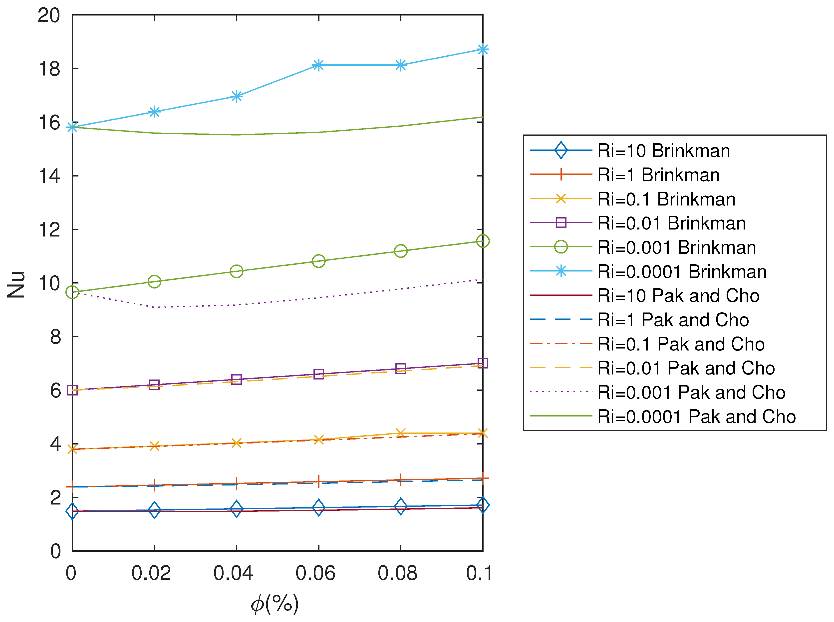
Figure 19 shows the average Nusselt number versus the nanoparticle volume fraction using the Brinkman and Pak formula for dynamic viscosity. For , the values of increase in line with the increase in nanoparticle volume fraction . When using the Brinkman model, the Nusselt number increases with increasing nanoparticle volume fraction . For the case when using the Pak formula, the Nusselt number shows a decrease initially when the nanoparticle volume fraction increases before recovering at larger concentrations. As compared to case A, the reduction in the Nusselt number for for the Pak and Cho model is much less for case B.
5. Conclusions
The mixed convective flow of a nanofluid in an enclosed square cavity with different boundary conditions was investigated. Two cases were studied: case A, in which the cavity’s top and bottom walls were kept at fixed temperatures, and the cavity’s left and right walls were maintained insulated, and case B, in which the left and right walls were kept at fixed temperatures and the top and bottom walls were insulated. In both cases, the top wall moved to the right at a fixed speed. The Brinkman model [12] and the Pak and Cho correlation [11] are two viscosity models that are used to estimate the viscosity of the nanofluid. The Pak and Cho correlation is obtained by fitting it with experimental data. Numerical results were obtained by solving the full Navier–Stokes equations using a single-phase model for the nanofluid, and a group of results were presented and discussed to demonstrate the effect of nanoparticle concentration and the Richardson number on flow and heat transfer behavior.
Heat transfer was demonstrated to increase significantly with the presence of nanoparticles, and this was greatly improved by increasing the nanoparticle volume fractions for large Richardson numbers (). However, the Pak–Cho model showed that the addition of nanoparticles would result in a decrease in the Nusselt numbers for small Richardson numbers (). This is also similar to the result found by Chamkha and Abu-Nada [16] in their studies.
Lid-driven cavity flow shows some classic features such as a large recirculating eddy in the main part of the cavity with secondary recirculating eddies near the corners. For large Reynolds numbers and decreasing Richardson numbers, the temperature, like the vorticity field, shows a region of constant values within the recirculating eddy in line with the Prandtl–Batchelor theorem. The features reported here have not been seen before because other investigators have not been able to compute the large Reynolds number solutions that we have successfully obtained with our different numerical techniques. When the particle concentration rises, it is apparent that the corner eddies are significantly more reduced with the Pak and Cho model than with the Brinkman model. This may be because the Pak and Cho viscosity model implies increased viscosities and, hence, reduced local Reynolds numbers as the particle concentration increases compared to the Brinkman model. The results are interesting because they suggest the potential of disrupting the formulation of recirculating eddies in the corner regions of the cavity by introducing nanoparticles into the flow. On the other hand, the Pak and Cho model would suggest less effective heat transfer properties, particularly for case A studied here. It is also noted that the Pak and Cho model solution is obtained by fitting with experimental data.
Our robust numerical techniques have also enabled novel solutions to be obtained for large Reynolds numbers and small Richardson numbers, parameter regimes where other numerical studies have encountered difficulties. In some of these cases, our results also interestingly show that there is a slight decrease in the Nusselt number and, hence, heat transfer properties for small particle concentrations, especially if the viscosity model used is one more closely aligned to fitted experimental data.
In this study, we focused primarily on a nanofluid based on water and Al2O3 nanoparticle mixtures, but similar results are expected for other nanofluid combinations. Other flow problems and configurations are studied in [21], where full details of the numerical techniques adopted in this paper are provided.
Finally, in our study, we used the single-phase model for the nanofluid. Whether similar results can be obtained using the two-phase model remains to be explored. The solution of the full equations, including those for the particle concentration, is non-trivial but worthy of further study.
Author Contributions
The work was equally shared out. J.S.B.G. was responsible for supervising the research. W.H.R.A. wrote the initial draft, J.S.B.G., the final draft. All authors have read and agreed to the published version of the manuscript.
Funding
This research received no external funding.
Institutional Review Board Statement
Not applicable.
Informed Consent Statement
Not applicable.
Data Availability Statement
The data can be made available upon request from the corresponding author.
Acknowledgments
The referees are thanked for their helpful comments. WA would like to thank the University of Hafr Al Batin for their support for this work and during her Ph.D. studies at Manchester University.
Conflicts of Interest
The authors declare no conflicts of interest.
References
- Choi, S.U.; Eastman, J.A. Enhancing Thermal Conductivity of Fluids with Nanoparticles; Technical report; Argonne National Lab.: Lemont, IL, USA, 1995. [Google Scholar]
- Eastman, J.A.; Choi, U.S.; Li, S.; Thompson, L.; Lee, S. Enhanced thermal conductivity through the development of nanofluids. MRS Online Proc. Libr. 1996, 457, 3–11. [Google Scholar] [CrossRef]
- Lee, S.; Choi, S.S.; Li, S.; Eastman, J. Measuring thermal conductivity of fluids containing oxide nanoparticles. ASME J. Heat Mass Transf. 1999, 121, 280–289. [Google Scholar] [CrossRef]
- Xie, H.; Wang, J.; Xi, T.; Liu, Y.; Ai, F.; Wu, Q. Thermal conductivity enhancement of suspensions containing nanosized alumina particles. J. Appl. Phys. 2002, 91, 4568–4572. [Google Scholar] [CrossRef]
- Das, S.K.; Putra, N.; Thiesen, P.; Roetzel, W. Temperature dependence of thermal conductivity enhancement for nanofluids. J. Heat Transf. 2003, 125, 567–574. [Google Scholar] [CrossRef]
- Sivashanmugam, P. Application of Nanofluids in Heat Transfer; Kazi, S.N., Ed.; InTechOpen: Rijeka, Croatia, 2012. [Google Scholar] [CrossRef]
- Cha, C.; Jaluria, Y. Recirculating mixed convection flow for energy extraction. Int. J. Heat Mass Transf. 1984, 27, 1801–1812. [Google Scholar] [CrossRef]
- Pilkington, L.A.B. Review lecture: The float glass process. Proc. R. Soc. Lond. A Math. Phys. Sci. 1969, 314, 1–25. [Google Scholar]
- Boutra, A.; Ragui, K.; Benkahla, Y.K. Numerical study of mixed convection heat transfer in a lid-driven cavity filled with a nanofluid. Mech. Ind. 2015, 16, 505. [Google Scholar] [CrossRef]
- Talebi, F.; Mahmoudi, A.H.; Shahi, M. Numerical study of mixed convection flows in a square lid-driven cavity utilizing nanofluid. Int. Commun. Heat Mass Transf. 2010, 37, 79–90. [Google Scholar] [CrossRef]
- Pak, B.C.; Cho, Y.I. Hydrodynamic and heat transfer study of dispersed fluids with submicron metallic oxide particles. Exp. Heat Transf. Int. J. 1998, 11, 151–170. [Google Scholar] [CrossRef]
- Brinkman, H.C. The viscosity of concentrated suspensions and solutions. J. Chem. Phys. 1952, 20, 571. [Google Scholar] [CrossRef]
- Arefmanesh, A.; Mahmoodi, M. Effects of uncertainties of viscosity models for Al2O3 water nanofluid on mixed convection numerical simulations. Int. J. Therm. Sci. 2011, 50, 1706–1719. [Google Scholar] [CrossRef]
- Maiga, S.E.B.; Nguyen, C.T.; Galanis, N.; Roy, G. Heat transfer behaviours of nanofluids in a uniformly heated tube. Superlattices Microstruct. 2004, 35, 543–557. [Google Scholar] [CrossRef]
- Sheikhzadeh, G.; Qomi, M.; Hajialigol, N.; Fattahi, A. Numerical study of mixed convection flows in a lid-driven enclosure filled with nanofluid using variable properties. Results Phys. 2012, 2, 5–13. [Google Scholar] [CrossRef]
- Chamkha, A.J.; Abu-Nada, E. Mixed convection flow in single-and double-lid driven square cavities filled with water–Al2O3 nanofluid: Effect of viscosity models. Eur. J. Mech.-B/Fluids 2012, 36, 82–96. [Google Scholar] [CrossRef]
- Ghafouri, A.; Salari, M.; Jozaei, A.F. Effect of variable thermal conductivity models on the combined convection heat transfer in a square enclosure filled with a water–alumina nanofluid. J. Appl. Mech. Tech. Phys. 2017, 58, 103–115. [Google Scholar] [CrossRef]
- Maxwell, J.C. A Treatise on Electricity and Magnetism; Oxford University Press: Oxford, UK, 1904. [Google Scholar]
- Azzam, N.A. Numerical Solution of the Navier-Stokes Equations for the Flow in a Lid-Driven Cavity and a Cylinder Cascade; University of Manchester: Manchester, UK, 2003. [Google Scholar]
- Alkahtani, B. Numerical Solutions to the Navier-Stokes Equations in Two and Three Dimensions. Ph.D. Thesis, The University of Manchester, Manchester, UK, 2013. [Google Scholar]
- Alruwaele, W. Study of Natural and Mixed Convection Flow of a Nanofluid. Ph.D. Thesis, The University of Manchester, Manchester, UK, 2023. [Google Scholar]
- Pereira, R.M.S.; Gajjar, J.S.B. Solving Fluid Dynamics Problems with Matlab. In Engineering Education and Research Using MATLAB; Assi, A.H., Ed.; InTech: Rijeka, Croatia, 2011. [Google Scholar] [CrossRef]
- Ghia, U.; Ghia, K.N.; Shin, C. High-Re solutions for incompressible flow using the Navier-Stokes equations and a multigrid method. J. Comput. Phys. 1982, 48, 387–411. [Google Scholar] [CrossRef]
Figure 1.
Schematic of the physical configuration for case A. The cavity has a width and height H. The top wall is a fixed temperature and the bottom wall has a fixed temperature . The shaded left and right walls are maintained in adiabatic conditions and the shading inside the cavity represents the nanoparticles. The top lid moves with speed to the right, whilst g denotes gravity.

Figure 2.
Schematic of the physical configuration for case B. The cavity has a width H and height H. The left wall is kept at a fixed temperature , and the right wall is kept at a fixed temperature . The shaded top and bottom walls are maintained in adiabatic conditions, and the shading inside the cavity represents the nanoparticles. The top wall moves with speed to the right.

Figure 3.
Comparison of the average Nusselt number with [16] at and for a single-lid-driven cavity for case A.
Figure 3.
Comparison of the average Nusselt number with [16] at and for a single-lid-driven cavity for case A.

Figure 4.
Contours of in subplots (a–c), in (g–i), and in (d–f) for case A using the Brinkman formula with and . Note that dotted contours have negative values.
Figure 4.
Contours of in subplots (a–c), in (g–i), and in (d–f) for case A using the Brinkman formula with and . Note that dotted contours have negative values.
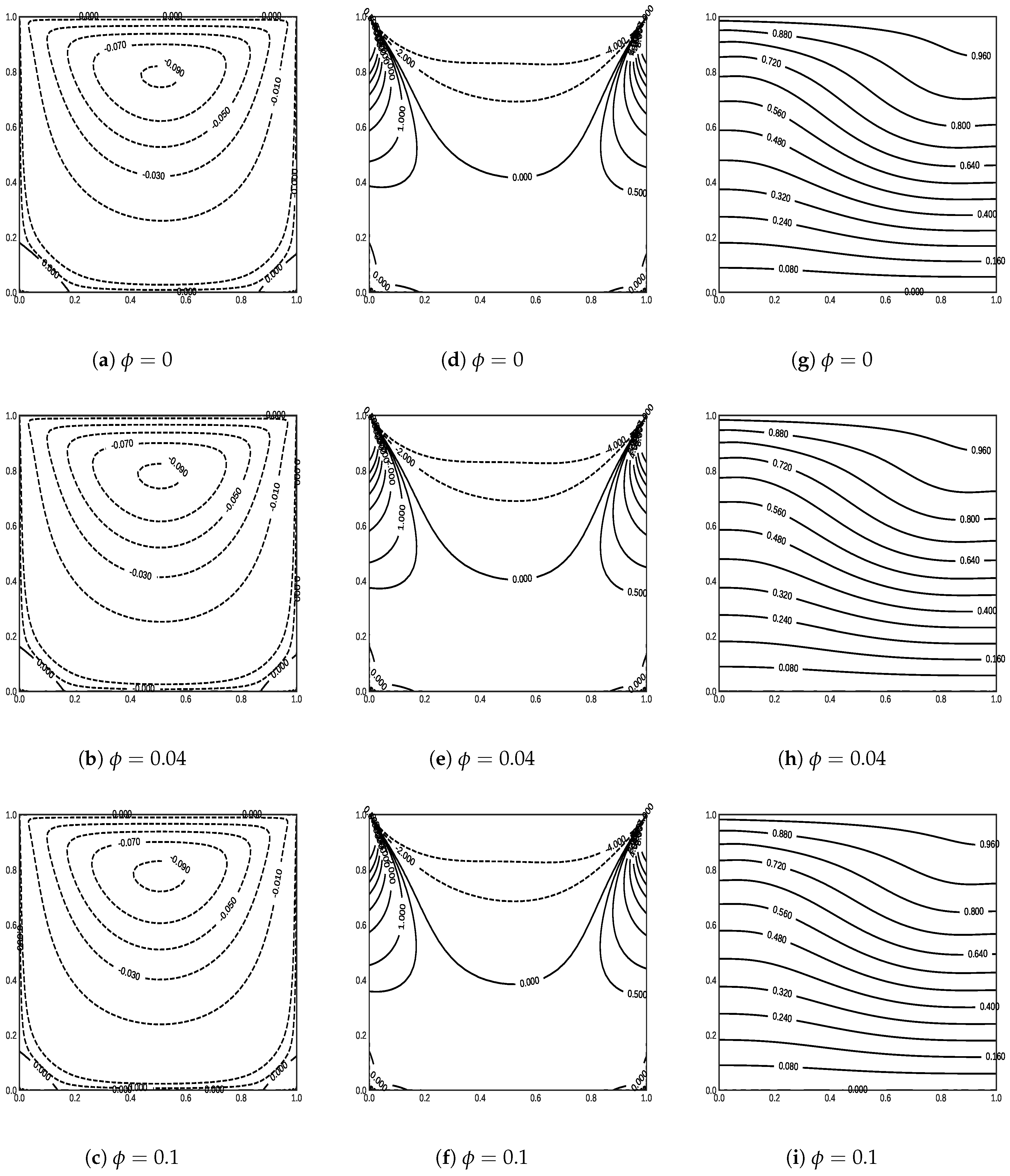
Figure 5.
Contours of in subplots (a–c), in (g–i), and in (d–f) for case A using the Pak and Cho correlation with and .
Figure 5.
Contours of in subplots (a–c), in (g–i), and in (d–f) for case A using the Pak and Cho correlation with and .

Figure 6.
Contours of in subplots (a–c), in (g–i), and in (d–f) for case A using the Brinkman formula with and .
Figure 6.
Contours of in subplots (a–c), in (g–i), and in (d–f) for case A using the Brinkman formula with and .
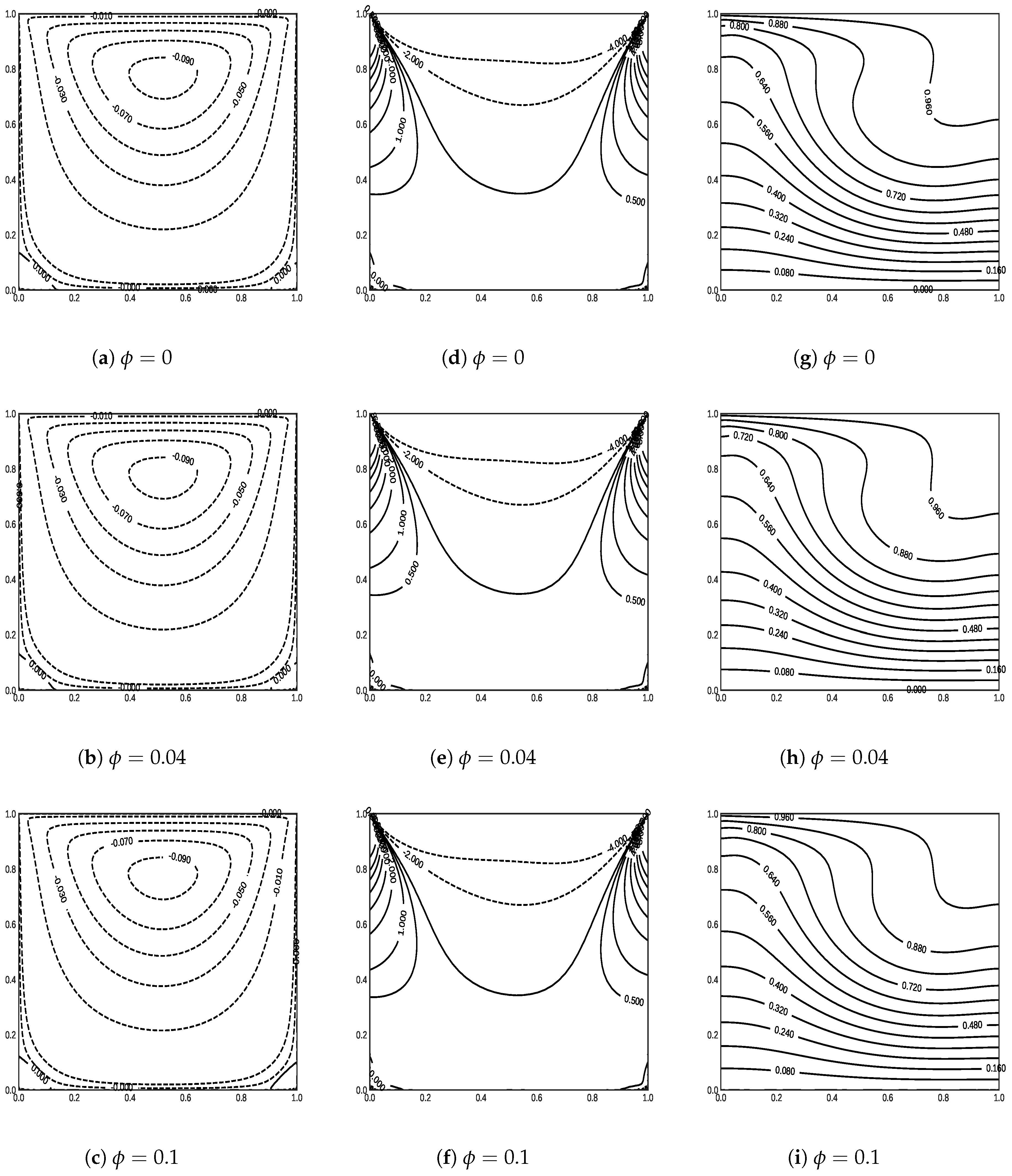
Figure 7.
Contours of in subplots (a–c), in (g–i), and in (d–f) for case A using the Pak and Cho correlation with and .
Figure 7.
Contours of in subplots (a–c), in (g–i), and in (d–f) for case A using the Pak and Cho correlation with and .

Figure 8.
Contours of in subplots (a–c), in (g–i), and in (d–f) for case A using the Brinkman formula with and .
Figure 8.
Contours of in subplots (a–c), in (g–i), and in (d–f) for case A using the Brinkman formula with and .

Figure 9.
Contours of in subplots (a–c), in (g–i), and in (d–f) for case A using the Pak and Cho correlation with and .
Figure 9.
Contours of in subplots (a–c), in (g–i), and in (d–f) for case A using the Pak and Cho correlation with and .
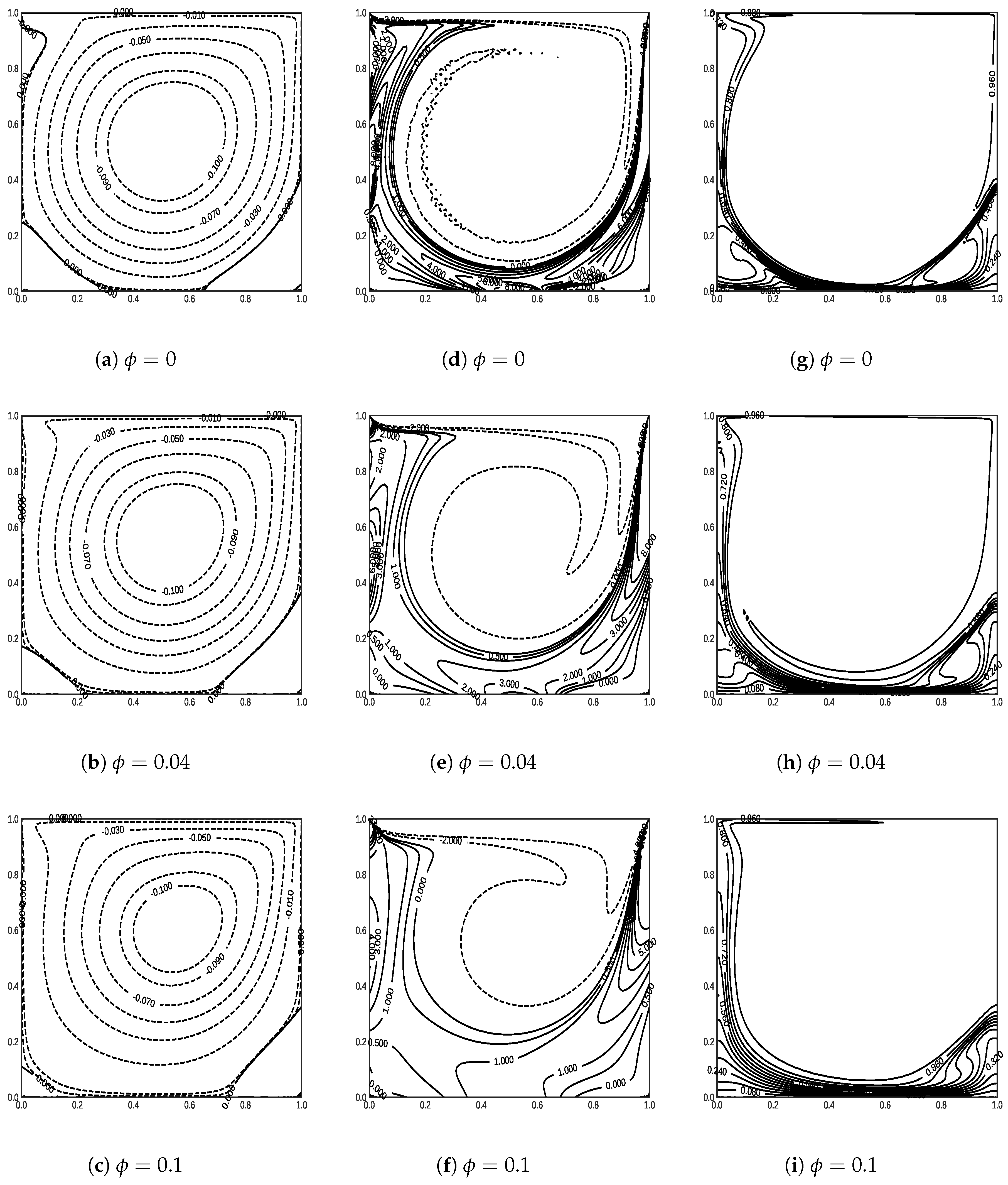
Figure 10.
Velocity profiles for u in subplots (a,b) and profiles of the temperature in (c,d) along a vertical line passing through the geometry center at and with Brinkman and Pak and Cho models.
Figure 10.
Velocity profiles for u in subplots (a,b) and profiles of the temperature in (c,d) along a vertical line passing through the geometry center at and with Brinkman and Pak and Cho models.

Figure 11.
Nusselt number versus particle concentrations for case A and with the two viscosity models for selected values of .
Figure 11.
Nusselt number versus particle concentrations for case A and with the two viscosity models for selected values of .

Figure 12.
Contours of the streamfunction in subplots (a–c), temperature in (g–i), and the vorticity in (d–f) for case B using the Brinkman formula with and .
Figure 12.
Contours of the streamfunction in subplots (a–c), temperature in (g–i), and the vorticity in (d–f) for case B using the Brinkman formula with and .
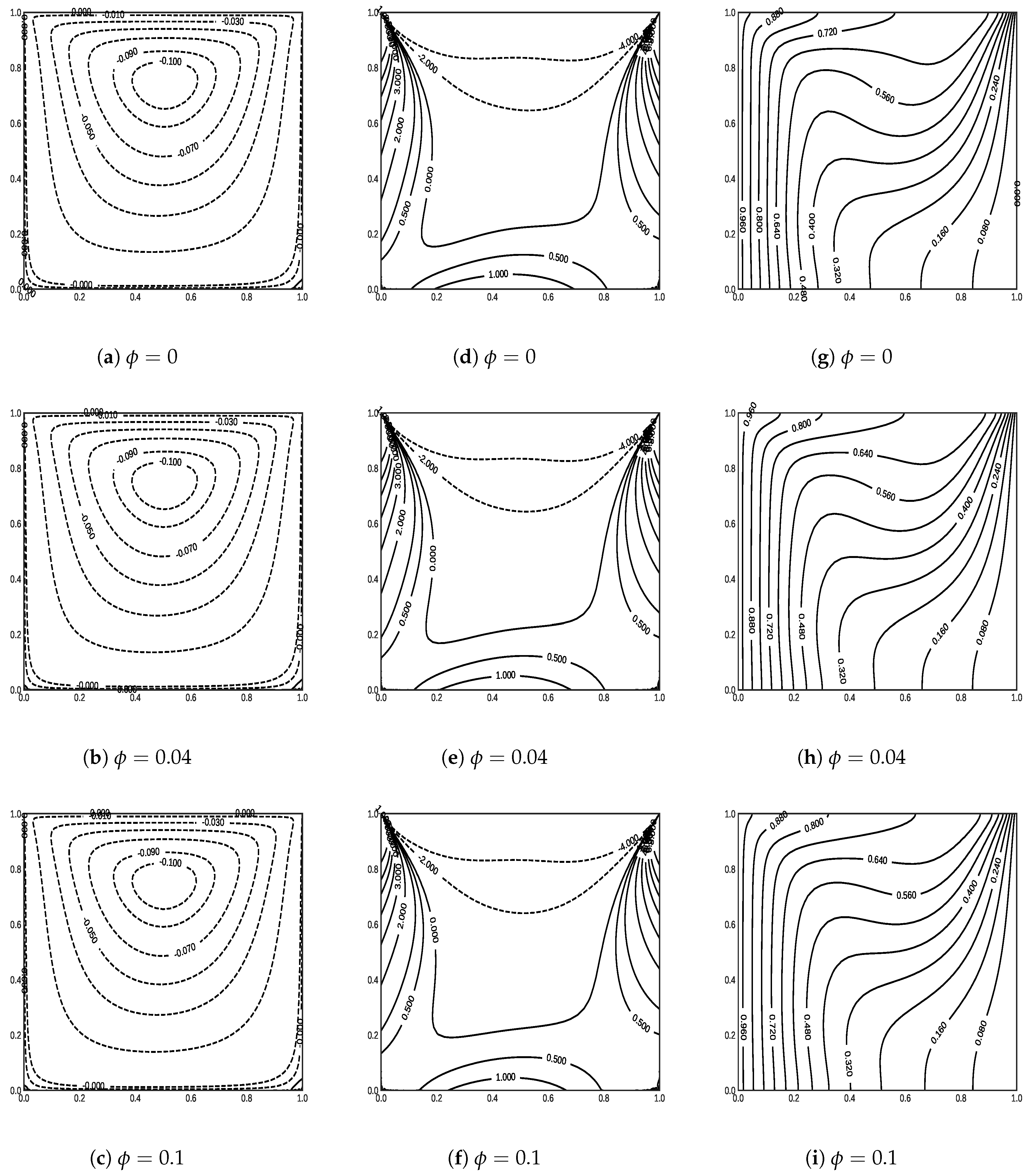
Figure 13.
Contours of the streamfunction in subplots (a–c), temperature in (g–i), and vorticity in (d–f) for case B using the Pak and Cho correlation with and .
Figure 13.
Contours of the streamfunction in subplots (a–c), temperature in (g–i), and vorticity in (d–f) for case B using the Pak and Cho correlation with and .

Figure 14.
Contours of the streamfunction in subplots (a–c), temperature in (g–i), and vorticity in (d–f) for case B using the Brinkman formula with and .
Figure 14.
Contours of the streamfunction in subplots (a–c), temperature in (g–i), and vorticity in (d–f) for case B using the Brinkman formula with and .

Figure 15.
Contours of the streamfunction in subplots (a–c), the temperature in (g–i), and vorticity in (d–f) for case B using the Pak and Cho correlation with and .
Figure 15.
Contours of the streamfunction in subplots (a–c), the temperature in (g–i), and vorticity in (d–f) for case B using the Pak and Cho correlation with and .

Figure 16.
Contours of the streamfunction in subplots (a–c), the temperature in (g–i), and vorticity in (d–f) for case B using the Brinkman formula with and .
Figure 16.
Contours of the streamfunction in subplots (a–c), the temperature in (g–i), and vorticity in (d–f) for case B using the Brinkman formula with and .
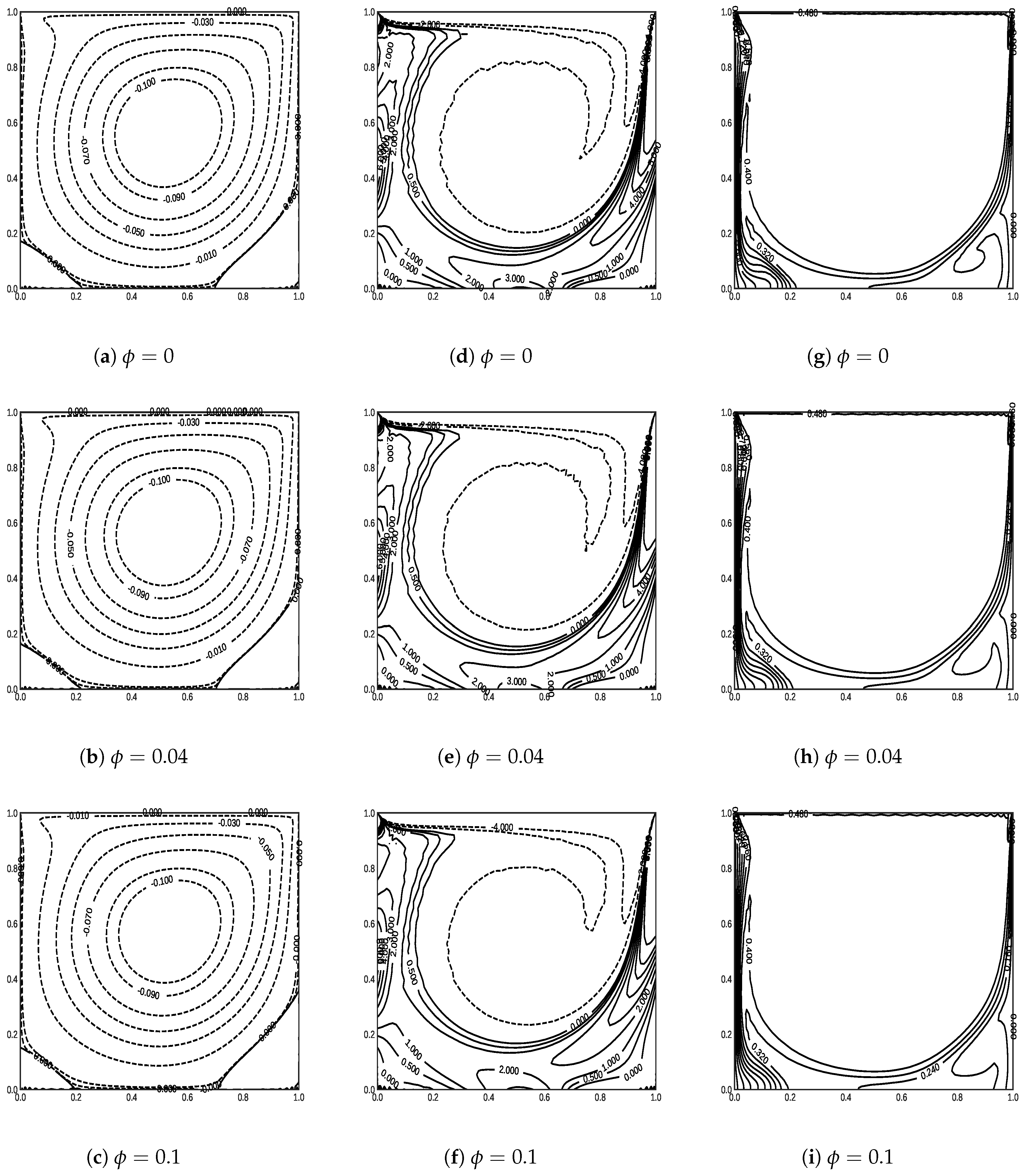
Figure 17.
Contours of the streamfunction in subplots (a–c), temperature in (g–i), and vorticity in (d–f) for case B using the Pak and Cho correlation with and .
Figure 17.
Contours of the streamfunction in subplots (a–c), temperature in (g–i), and vorticity in (d–f) for case B using the Pak and Cho correlation with and .

Figure 18.
Profiles of the velocity in (a,b) and temperature in (c,d) along a vertical line passing through the geometry center at and with the Brinkman and Pak and Cho models.
Figure 18.
Profiles of the velocity in (a,b) and temperature in (c,d) along a vertical line passing through the geometry center at and with the Brinkman and Pak and Cho models.

Figure 19.
Nusselt number for case B for selected Richardson numbers.

Table 1.
Thermophysical properties of the base fluid and nanoparticles.
| Property | Base Fluid | Nanoparticles |
|---|---|---|
| Specific Heat (J/kg/K) | 4179 | 765 |
| Density (kg/m3) | 997.1 | 3970 |
| Thermal Conductivity k (W/mK) | 0.613 | 25 |
| Dynamic Viscosity (Ns m−2) | 8.91 × | |
| Thermal Conductivity coefficient (1/K) | 2.1 × | 8.5 × |
Table 2.
Minimum values of the function for case A using the Brinkman and Pak and Cho formulae at selected Richardson numbers.
Table 2.
Minimum values of the function for case A using the Brinkman and Pak and Cho formulae at selected Richardson numbers.
| Brinkman (Ri = 10) | Pak and Cho (Ri = 10) | Brinkman (Ri = 0.00001) | Pak and Cho (Ri = 0.00001) | |
|---|---|---|---|---|
| 0 | −0.091846174 | −0.0918462 | −0.122128526 | −0.122128526 |
| 0.02 | −0.092820132 | −0.095179 | −0.122150678 | −0.120607855 |
| 0.04 | −0.092476482 | −0.0967305 | −0.122160357 | −0.119011494 |
| 0.06 | −0.092820132 | −0.0975358 | −0.122158149 | −0.117359139 |
| 0.08 | −0.093175107 | −0.0979984 | −0.122144814 | −0.115609126 |
| 0.1 | −0.09353645 | −0.0982861 | −0.122121257 | −0.113943122 |
Table 3.
Minimum values of the streamfunction for case B using the Brinkman and Pak and Cho formulae at selected Richardson numbers.
Table 3.
Minimum values of the streamfunction for case B using the Brinkman and Pak and Cho formulae at selected Richardson numbers.
| Brinkman (Ri = 10) | Pak (Ri = 10) | Brinkman (Ri = 0.0001) | Pak (Ri = 0.0001) | |
|---|---|---|---|---|
| 0 | −0.118110653 | −0.1181107 | −0.12117914 | −0.12117914 |
| 0.02 | −0.118396409 | −0.1094735 | −0.121281759 | −0.115927735 |
| 0.04 | −0.118559806 | −0.1054175 | −0.121326906 | −0.112511571 |
| 0.06 | −0.118604327 | −0.1032767 | −0.121326906 | −0.10953728 |
| 0.08 | −0.118534614 | −0.1020207 | −0.121254546 | −0.107110616 |
| 0.1 | −0.118356374 | −0.1012208 | −0.171907578 | −0.105025779 |
Disclaimer/Publisher’s Note: The statements, opinions and data contained in all publications are solely those of the individual author(s) and contributor(s) and not of MDPI and/or the editor(s). MDPI and/or the editor(s) disclaim responsibility for any injury to people or property resulting from any ideas, methods, instructions or products referred to in the content. |
© 2024 by the authors. Licensee MDPI, Basel, Switzerland. This article is an open access article distributed under the terms and conditions of the Creative Commons Attribution (CC BY) license (https://creativecommons.org/licenses/by/4.0/).
Share and Cite
MDPI and ACS Style
Alruwaele, W.H.R.; Gajjar, J.S.B. Lid-Driven Cavity Flow Containing a Nanofluid. Dynamics 2024, 4, 671-697. https://doi.org/10.3390/dynamics4030034
AMA Style
Alruwaele WHR, Gajjar JSB. Lid-Driven Cavity Flow Containing a Nanofluid. Dynamics. 2024; 4(3):671-697. https://doi.org/10.3390/dynamics4030034
Chicago/Turabian StyleAlruwaele, Wasaif H. R., and Jitesh S. B. Gajjar. 2024. "Lid-Driven Cavity Flow Containing a Nanofluid" Dynamics 4, no. 3: 671-697. https://doi.org/10.3390/dynamics4030034