Abstract
Tropical cyclones (TCs) can be characterized as a 3D annular structure of elevated potential vorticity (PV). However, strong mature TCs often develop a secondary eyewall, leading to a 3D annular vortex with a double-eyewall structure. Using 2D linear stability analysis, it is shown that three types of barotropic instability (BI) are present for annular vortices with a double-eyewall structure: Type-1 BI across the secondary eyewall, Type-2 BI across the moat of the vortex, and Type-3 BI across the primary eyewall. The overall stability of these vortices (and the type of BI that develops) depends principally upon five vortex parameters: the thickness of the primary eyewall, the thickness of the secondary eyewall, the moat width, the vorticity ratio between the eye and the primary eyewall, and the vorticity ratio between the primary and secondary eyewall. The adiabatic evolution of 3D annular vortices with a double-eyewall structure is examined using a primitive equation model in normalized isobaric coordinates. It is shown that Type-2 BI is the most common type of BI for 3D annular vortices whose vortex parameters mimic TCs with a double-eyewall structure. During the onset of Type-2 BI, eddy kinetic energy budget analysis indicates that barotropic energy conversion from the mean azimuthal flow is the dominant energy source of the eddies, which produces a radial velocity field with a quadrupole structure. Absolute angular momentum budget analysis indicates that Type-2 BI generates azimuthally averaged radial outflow across the moat, and the eddies transport absolute angular momentum radially outward towards the secondary eyewall. The combination of these processes leads to the dissipation of the primary eyewall and the maintenance of the secondary eyewall for the vortex.
1. Introduction
It has been shown that asymmetric processes within the core of tropical cyclones (TCs) have a large impact on the structure and evolution of TCs [1,2,3,4,5]. The dynamical evolution of the TC inner core can be explained by using a potential vorticity (PV) framework. For fully three-dimensional motions including diabatic and frictional sources, the evolution of PV is given by the Rossby–Ertel PV equation:
where D/Dt is the total (material) derivative, is the specific volume, is the absolute vorticity vector, is the potential temperature, is the diabatic heating rate, is the potential vorticity, and is the frictional force per unit mass. Within the inner core of a mature TC, the absolute vorticity vector points radially outward and upwards. Since obtains its maximum value within the middle troposphere, air parcels flowing inward within the lower troposphere and spiraling upward in the eyewall experience an increase in PV due to diabatic heating. PV is then advected vertically into the upper troposphere, producing a towering annular structure of elevated PV (known as a hollow PV tower). The hollow PV tower extends from the lower to middle troposphere with values of PV as high as 275 PV units (where 1 PV unit = ) [6,7].
Since the radial structure of the hollow PV tower satisfies the Charney–Stern condition for combined barotropic–baroclinic instability [8,9], the hollow PV tower may break down, causing PV mixing between the eyewall and the eye. The instability of the eyewall and the subsequent PV mixing within the inner core of the TC has been examined extensively in idealized numerical modeling frameworks [3,10,11,12,13,14,15,16,17,18,19,20,21,22], in full-physics numerical modeling [23,24,25,26,27,28,29], and in observational and experimental studies [30,31,32,33,34,35]. In the absence of diabatic heating and frictional effects, PV is conserved, and the annular vortex structure leads to barotropic instability (BI) within the inner core of the vortex. In addition to the strength of the annular vortex, the subsequent evolution of the hollow PV tower depends upon the hollowness of the vortex (i.e., the ratio of eye to inner-core PV) and the eyewall thickness of the vortex (i.e., the ratio of the inner and outer radii of the eyewall of the annular vortex) [10,11]. When the effects of diabatic heating are included, BI (and the subsequent PV mixing) functions as a transient brake in intensification [20,22]. Moreover, diabatic heating produces a strengthening and thinning of the hollow PV tower structure due to the combined effects of radial PV advection and diabatic heating [12,22]. In contrast, friction is shown to stabilize the hollow PV tower structure by reducing eyewall PV and the unstable barotropic growth rate [12].
The previously mentioned studies examined the evolution of a 3D annular vortex structure which mimicked a mature TC with a single eyewall. However, numerous aircraft and satellite observations have shown that mature TCs frequently develop a secondary wind maximum outside of the primary eyewall, which is known as secondary eyewall formation [1,36]. Since a secondary eyewall in a TC is accompanied by a ring of convection [37], this implies that the radial structure of a mature TC with a primary and secondary eyewall can also be examined using a PV framework. Similar to the argument made above, a mature TC with a double-eyewall structure consists of a central region with low PV, a towering structure of elevated PV that corresponds to the primary eyewall, a local minimum in PV that corresponds to the moat, and a local maximum in PV that corresponds to the secondary eyewall.
The development of a secondary eyewall in a mature TC usually leads to an eyewall replacement cycle (ERC) in which the secondary eyewall typically contracts and intensifies, while the primary eyewall weakens, dissipates, and is replaced by the secondary eyewall [38,39]. This cycle often produces an oscillation of TC intensity, and it is usually accompanied by an expansion of the TC wind field. Although the ERC is well documented, there have been relatively few studies that have examined the dynamical processes associated with the evolution of a double-eyewall vortex. Ref. [40] used a 2D non-divergent barotropic model to examine the evolution of a 2D vortex composed of a central, monopolar vortex with an annular ring of vorticity, and it was shown that two types of instability are present:
- Type-1 BI occurs across the secondary eyewall when the secondary eyewall is sufficiently narrow and when the circulation associated with the primary eyewall is too weak to stabilize the secondary eyewall.
- Type-2 BI occurs across the moat when the radial extent of the moat (i.e., the moat width) is narrow enough so that unstable interactions occur between the primary eyewall and the inner edge of the secondary eyewall.
Refs. [41,42] examined the evolution of a 2D annular vortex with a double-eyewall structure using a shallow water framework, and it was shown that Type-2 BI makes a significant contribution to the dissipation of the primary eyewall through eddy radial transport of absolute angular momentum. Furthermore, it was shown that Type-2 BI can increase the absolute angular momentum of the secondary eyewall.
The purpose of the present study is to extend the analysis of Refs. [40,41,42] in two ways. First, as noted in Ref. [41], a 2D annular vortex with a double-eyewall structure satisfies the Rayleigh necessary condition for BI across the primary eyewall, the moat region, and the secondary eyewall. Using 2D linear stability analysis, it will be shown that the type of BI that develops for a 2D annular vortex with a double-eyewall structure (along with the fastest growing mode and its PV growth rates) depends principally upon five vortex parameters: the thickness of the primary eyewall, the thickness of the secondary eyewall, the moat width, the vorticity ratio between the primary and secondary eyewall, and the vorticity ratio between the eye and the primary eyewall. Second, this study will extend the analysis of Refs. [40,41,42] to the next level of complexity towards the real atmosphere by using a three-dimensional primitive equation model. This work will examine how each type of BI affects the evolution of 3D annular vortices with a double-eyewall structure. Eddy kinetic energy budget analysis will be used to examine the role of eddy processes in the evolution of these vortices, whereas angular momentum budget analysis will be used to examine the processes that contribute to the intensity change in the primary and secondary eyewall. For 3D vortices that mimic TCs with a double-eyewall structure, it will be shown that the formation and growth of eddies associated with the onset of BI contributes to the dissipation of the primary eyewall.
This paper is organized in the following manner. In Section 2, the linear stability analysis associated with the 2D annular vortex with a double-eyewall structure is presented. In Section 3, the primitive equation model along with the initial conditions used in this study is presented, and the nonlinear PV evolution for the control experiment is discussed. In Section 4, sensitivity experiments are presented to investigate how changes in the vortex parameters associated with the initial condition of the vortex impact the nonlinear evolution of PV for the 3D annular vortex with a double-eyewall structure. Conclusions are given in Section 5.
2. Linear Stability Analysis
2.1. Derivation
To examine the types of BI that are present during the evolution of a 2D annular vortex with a double-eyewall structure, the linearized 2D non-divergent barotropic vorticity equation in polar coordinates is used.
where is the axisymmetric vertical vorticity, is the axisymmetric angular velocity, and is the perturbation streamfunction. Assuming wave solutions of the form where is the azimuthal wavenumber and is the frequency, Equation (2) can be rewritten as follows:
To solve Equation (3), we must specify the axisymmetric vertical vorticity. To model a 2D annular vortex with a double-eyewall structure, the vortex model of Ref. [41] has been extended into a six-region model which consists of an eye region (region 1), an annular primary eyewall region (region 2), a moat region (region 3), an annular secondary eyewall region (region 4), an outer vortex region with small vorticity (region 5), and a far-field vortex region with zero vorticity (region 6), as shown in Figure 1. This six-region model can be written mathematically as follows:
where , , , , and are the specified radii and , , , , and are the specified vertical vorticity values for each region.
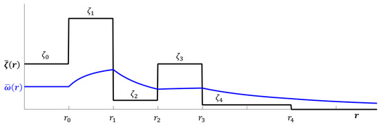
Figure 1.
Schematic of the axisymmetric vertical vorticity (with solid black curve) for the six-region 2D annular vortex with a double-eyewall structure. The accompanying angular velocity is given by the solid blue curve.
Since each piecewise region in Equation (4) has constant vertical vorticity, as shown in Figure 1, everywhere except at , , , , and . Therefore, Equation (3) reduces to the following:
which is valid for all six regions. Since Equation (5) has the form of Euler’s differential equation, its general solution in the six regions can be constructed from different linear combinations of and in each region. Thus, the general solution can be written as follows:
where , , , , and are complex coefficients. Following Ref. [39], the complex coefficients can be related by integrating Equation (3) over the narrow radial regions centered at , , , , and to obtain the following:
where , , and . Substituting Equation (6) into Equation (7) and dividing by produces the following eigenvalue equation:
where is the non-dimensional wave growth rate and is a non-dimensional matrix associated with the axisymmetric vorticity . The full form of can be found in the Appendix A, and it is a function of eight non-dimensional parameters:
- is the ratio of the eye to primary eyewall vorticity. Following Ref. [10], will be called the hollowness of the vortex.
- is the ratio of the primary to second eyewall vorticity. will be called the eyewall vorticity ratio.
- is the ratio of the moat vorticity to secondary eyewall vorticity. will be called the moat strength.
- is the ratio of the far-field vorticity to secondary eyewall vorticity. Since the vorticity of the outer vortex is usually denoted as the vortex skirt [43], will be called the skirt strength.
- is the ratio of the inner to outer primary eyewall radius. Notice that, as approaches 1, the primary eyewall thins. For this reason, will be called the primary eyewall thickness. It will be shown in Section 2.2 that this parameter plays an important role in the onset of BI across the primary eyewall of the vortex, which is known as Type-3 BI.
- is the ratio of the outer primary eyewall radius to the inner secondary eyewall radius. Notice that, as increases (with all other parameters held constant), decreases. Furthermore, notice that implies that . This means that is a measure of the radial extent of the moat such that values of close to 1 correspond to a vortex with a small moat and values of close to 0 correspond to a vortex with a large moat. For this reason, will be called the moat width parameter. It will be shown in Section 2.2 that this parameter plays an important role in the onset of Type-2 BI.
- is the ratio of the inner to outer secondary eyewall radius. Notice that, as approaches 1, the secondary eyewall thins. For this reason, will be called the secondary eyewall thickness. It will be shown in Section 2.2 that this parameter plays an important role in the onset of Type-1 BI.
- is the ratio of the outer secondary eyewall radius to the radius of the outer vortex. Notice that, as increases (with all other parameters held constant), decreases. Furthermore, notice that implies that . This means that is a measure of the radial extent of the skirt such that corresponds to a vortex with no skirt and corresponds to a vortex whose skirt extends through the entire far-field region of the vortex. For this reason, will be called the skirt width.
The eigenvalue equation in Equation (8) is solved by evaluating the following determinant equation:
where is a identity matrix. For a given value of the azimuthal wavenumber along with the eight parameters defined above, a solution to Equation (9) gives five values for the non-dimensional wave growth rate , and the most unstable value from these roots (which corresponds to the fastest growing mode) is chosen for each . The most unstable mode is identified as the mode in which the azimuthal wavenumber has the largest wave growth. For this manuscript, corresponds to the azimuthal wavenumber associated with the most unstable mode.
To complete the linear stability analysis, the parameter range of eight vortex parameters must be defined. For annular vortices with a double-eyewall structure, the range of , , , , , , and is between 0 and 1. Although can range from 0 to , the range of was set to between 0 and 5 in order to mimic TCs with a double-eyewall structure [39]. Equation (9) was solved for the most unstable mode (with its the non-dimensional growth rate) for this parameter space with increments of 1/60. Based on the description of the eight parameters given above, it is not expected that each parameter will have a significant influence on the stability of the vortex. To understand why this should be the case, it is important to note that the most unstable mode results from the mutual growth of vortex Rossby waves (VRWs) associated with various regions within the vortex. The theory of VRWs suggests that only the core of the vortex can support VRWs [43], which implies that and should play negligible roles in the linear stability of the vortex. It can be shown that the stability of the vortex is largely independent of and , except when (which corresponds to the scenario where the secondary eyewall vorticity is greater than the primary eyewall vorticity). In the following section, the effects of , , , , , and on the linear stability of the vortex will be given.
2.2. Results from Linear Stability Analysis
Figure 2 examines the impact of the primary eyewall thickness , the moat width , and the secondary eyewall thickness on the stability of the vortex. For (which corresponds to a thick secondary eyewall), there are three important patterns to note. First, for (which corresponds to a large moat width), the vortex is stable for (which corresponds to a thick primary eyewall), as shown in Figure 2a,b. Thus, the linear analysis indicates that the 2D annular vortex is stable for thick eyewalls with a large moat region. Second, as increases beyond 0.500, note that the azimuthal wavenumber associated with the most unstable mode increases from to , and the wave growth rates increase as increases, as shown in Figure 2a–c. Since controls the thickness of the primary eyewall, increasing excites an instability across the primary eyewall. As mentioned in Section 2.1, this instability is known as a Type-3 BI, which results from phase-locked VRWs across the primary eyewall [3,41]. Third, as increases beyond 0.500, note that the azimuthal wavenumber associated with the most unstable mode increases from to , and the wave growth rates increase as increases, as shown in Figure 2c,d. Since controls the moat width, increasing excites an instability across the moat of the vortex. As mentioned in Section 1, this instability is known as a Type-2 BI, which results from the mutual growth of VRWs across the moat [41].
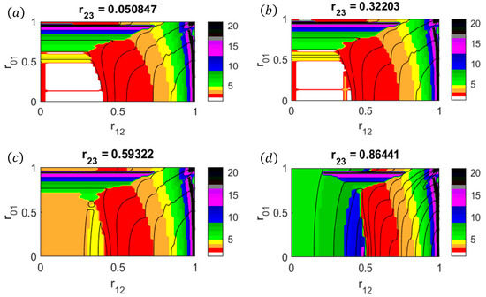
Figure 2.
Isolines of the dimensionless growth rate computed from Equation (9) as a function of primary eyewall thickness and moat width . The minimum isoline value is , and the contour interval is 0.05. The color shading indicates the azimuthal wavenumber associated with the most unstable mode where the white color indicates the stable region. For each panel, , , , , and .
Finally, Figure 2 also demonstrates the impact of increasing on the stability of the vortex. As exceeds 0.500, the azimuthal wavenumber associated with the most unstable mode increases from to in the parameter range and , and the wave growth rates increase as increases. Since controls the thickness of the secondary eyewall, increasing excites an instability across the secondary eyewall. This instability is known as a Type-1 BI, which results from phase-locked VRWs across the secondary eyewall [3,41]. (Figure 2, Figure 3, Figure 4, Figure 5, Figure 6 and Figure 7 describe the parameter range for the most unstable mode. This should not be interpreted to mean that only one type of BI is present for a given parameter range. Multiple type of barotropic instability can coexist in the same vortex for a given parameter range, although their unstable wave growth rates will be different. This will play an important role in the interpretation of 3D annular vortices given in Section 4.)
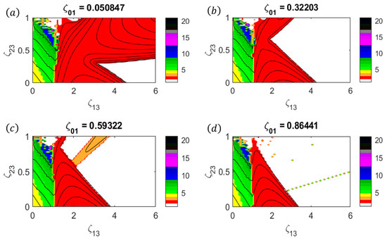
Figure 3.
Isolines of the maximum value of the dimensionless growth rate computed from Equation (9) as a function of eyewall vorticity ratio and the moat strength f. The minimum isoline value is , and the contour interval is 0.05. The color shading indicates the azimuthal wavenumber associated with the most unstable mode where the white color indicates the stable region. For each panel, , , , , and .
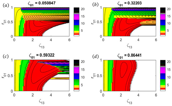
Figure 4.
Isolines of the maximum value of the dimensionless growth rate computed from Equation (9) as a function of eyewall vorticity ratio and primary eyewall thickness The minimum isoline value is , and the contour interval is 0.05. The color shading indicates the azimuthal wavenumber associated with the most unstable mode where the white color indicates the stable region. For each panel, , , , , and .
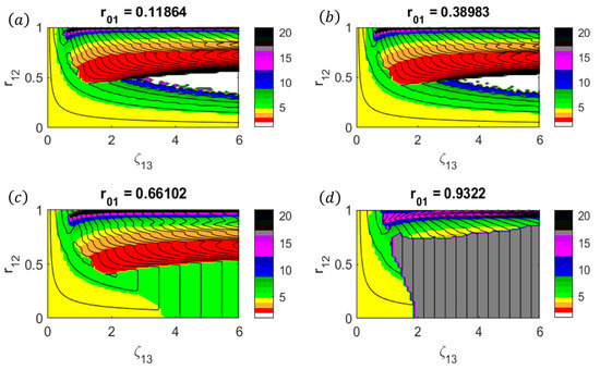
Figure 5.
Isolines of the maximum value of the dimensionless growth rate computed from Equation (9) as a function of eyewall vorticity ratio and moat width . The minimum isoline value is , and the contour interval is 0.05. The color shading indicates the azimuthal wavenumber associated with the most unstable mode where the white color indicates the stable region. For each panel, , , , , and .
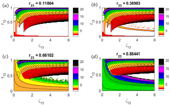
Figure 6.
Isolines of the maximum value of the dimensionless growth rate computed from Equation (9) as a function of eyewall vorticity ratio and moat width . The minimum isoline value is , and the contour interval is 0.05. The color shading indicates the azimuthal wavenumber associated with the most unstable mode where the white color indicates the stable region. For each panel, , , , , and .
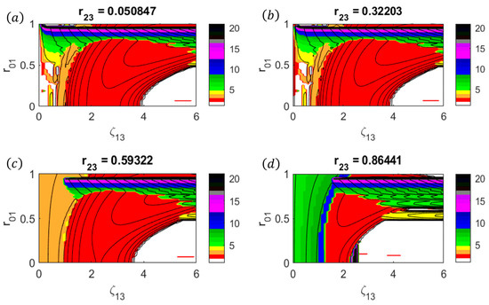
Figure 7.
Isolines of the maximum value of the dimensionless growth rate computed from Equation (9) as a function of eyewall vorticity ratio and primary eyewall thickness . The minimum isoline value is , and the contour interval is 0.05. The color shading indicates the azimuthal wavenumber associated with the most unstable mode where the white color indicates the stable region. For each panel, , , , , and .
Figure 3 examines the impact of the vortex hollowness , the eyewall vorticity ratio , and the moat strength on the stability of the vortex. The parameters , , , and were chosen such that Type-1 or Type-2 BI could be excited. It should be noted that there is a clear distinction in the behavior of the vortex when (i.e., in which the secondary eyewall is stronger than the primary eyewall) compared to (i.e., in which the primary eyewall is stronger than the secondary eyewall). In the parameter region , Type-1 BI is excited with for small and for small , as shown in Figure 3a–d (i.e., which corresponds to a hollow vortex with small moat vorticity). As increases, the azimuthal wavenumber corresponding to the most unstable mode for the Type-1 BI increases from to . Physically, and correspond to a scenario in which the secondary eyewall has virtually replaced the primary eyewall. In contrast, for the parameter region and (which corresponds to a hollow vortex with a strong primary eyewall), Type-2 BI is excited with for all values of , as shown in Figure 3a–d. These results suggest that the moat vorticity plays a relatively unimportant role in the dynamics when (i.e., the primary eyewall is stronger than the secondary eyewall). Finally, it should be noted that the vortex becomes stable for large and large , as shown in Figure 3c,d. Physically, this corresponds to a strong, filled vortex with a thin secondary eyewall, and as shown in Ref. [40], the circulation of a strong, central vortex can induce enough differential rotation across the outer ring to prevent Type-1 BI.
Figure 2 illustrates that different types of barotropic instabilities are present based upon the thickness of the eyewalls and their relative positions through the moat width. We will now examine how changes in the eyewall vorticity and moat strength lead to the onset of different types of BI. Figure 4 examines the impact of the vortex hollowness , the eyewall vorticity ratio , and the moat strength on the stability of the vortex. First, it should be noted that the vortex hollowness plays an unimportant role when , which corresponds to a thick primary eyewall with a small eye. As increases within the parameter range , the behavior of the vortex is similar to Figure 3c in which the vortex is unstable with Type-2 BI with for , unstable with Type-2 BI with for , and stable for . Similar to Figure 2b, there is an overlap of Type-2 and Type-3 BI in the parameter range , , and , as shown in Figure 4a,b. However, as increases within the parameter range , notice that the Type-3 BI is removed, as shown in Figure 4c,d. Similar to the argument made above, the differential rotation across the primary eyewall can prevent the onset of Type-3 BI. Similarly, as and increase within the parameter range , notice that both Type-2 and Type-3 BI are removed, as shown in Figure 4d. In other words, very large and are required to stabilize the vortex when the primary eyewall is very thin.
Figure 5 examines the impact of moat width , primary eyewall thickness , and eyewall vorticity ratio on the development of each type of BI. For (i.e., large moat width) and small (i.e., large primary eyewall thickness), the vortex is dominated by Type-1 BI, as shown in Figure 5a,b Interestingly, the vortex is stable for the parameter range , , and . In other words, a relatively wide moat with a strong primary eyewall is a stable vortex, as discussed in Figure 3. As increases (i.e., moat width decreases) for a fixed in which , there is a transition from Type-1 BI to Type-2 BI, as shown in Figure 5a,b. However, it should be noted that this transition occurs only for . Thus, Type-1 BI occurs across the secondary eyewall for sufficiently thin and strong secondary eyewalls. As shown in Figure 5c,d, Type-3 BI dominates the dynamics within the parameter range , , and .
Figure 6 examines the impact of moat width , secondary eyewall thickness , and eyewall vorticity ratio on the development of Type-1 and Type-2 BI. For the parameter range and (which corresponds to thick primary and secondary eyewalls), the vortex is stable for virtually all values of , as shown in Figure 6a. As increases, a Type-2 BI begins to develop with increasing growth rates, as shown in Figure 6a,b, whereas as increases, a Type-1 BI develops with increasing growth rates for , as shown in Figure 6c,d. It is important to note that the transition from Type-1 BI to Type-2 BI occurs within the parameter range and , as shown in Figure 6c,d. This implies that the relative strength between the primary eyewall and the secondary eyewall determines the type of BI present in 3D annular vortices.
Finally, Figure 7 examines the impact of primary eyewall thickness , eyewall vorticity ratio , and secondary eyewall thickness on the stability of the vortex. Notice that large and small (i.e., thick primary eyewalls) lead to a stable vortex regardless of . As shown in Figure 7a,b, increasing above 0.7 (which corresponds to thin primary eyewalls) excites Type-3 BI for small values of . As shown in Figure 7c,d, Type-1 BI is excited within the parameter range and , which corresponds to strong secondary eyewalls. In contrast, for , Type-2 BI is excited for and , as shown in Figure 7a–c. In general, when the primary eyewall dominates (which occurs when ), changes in secondary eyewall thickness do not impact the dynamics except for very thin secondary eyewalls (i.e., when ). This describes the transition from Type-2 BI to Type-1 BI.
In summary, although the linear stability analysis indicates that eight vortex parameters are needed to specify the fastest growing mode for 2D annular vortices with a double-eyewall structure, as defined by Equation (4), the five principal vortex parameters are the primary eyewall thickness , the moat width parameter , the secondary eyewall thickness , the vortex hollowness , and the eyewall vorticity ratio . In general, there are four important trends that can be deduced from the numerical solutions associated with the linear stability analysis:
- The parameter range in which the vortex is stable is , , , and . Physically, this corresponds to a 2D annular vortex with a thick primary eyewall, a large moat, and a weak secondary eyewall.
- The parameter range in which Type-1 BI is excited across the secondary eyewall is , , , and . Physically, this corresponds to a 2D annular vortex with a thick primary eyewall, a large moat, and a strong, thin secondary eyewall. As shown in Figure 2 and Figure 5, Type-1 BI can be excited even for relatively weak secondary eyewalls if the secondary eyewall is sufficiently thin (i.e., ). In general, as increases, Type-1 BI is excited with increasingly large azimuthal wavenumbers. In contrast, Type-1 BI can be removed by increasing the circulation associated with the central vortex via and (as shown in Figure 3 and Figure 4).
- The parameter range in which Type-2 BI is excited across the moat of the vortex is , , and . Physically, this corresponds to a 2D annular vortex with a small moat and a relatively weak secondary eyewall. As shown in Figure 2, Figure 5 and Figure 6 Type-2 BI can be excited even for thin secondary eyewalls and/or thin primary eyewalls if the moat width is sufficiently small (i.e., ).
- The parameter range in which Type-3 BI is excited across the primary eyewall is , , , , and . Physically, this corresponds to a 2D annular vortex with a thin, strong primary eyewall, a large moat, and a weak secondary eyewall. As shown in Figure 5, Type-1 BI can be excited for thin secondary eyewalls only if the primary eyewall is sufficiently thin (i.e., ) and if the primary eyewall is sufficiently strong (i.e., ). In contrast, Type-1 BI can be removed by increasing the hollowness parameter, as shown in Figure 4. The transition between Type-1 and Type-3 BI is strongly governed by the eyewall vorticity ratio . Type-1 BI plays an important role in the dynamics for , whereas Type-3 BI plays an important role in the dynamics for .
As discussed in the summary above, the onset of Type-3 BI requires the most restrictive parameter range for 2D annular vortices with a double-eyewall structure, whereas the onset of Type-2 BI requires the least restrictive parameter range. In the following sections, we will use the framework discussed in this section to examine the adiabatic evolution of 3D annular vortices with a double-eyewall structure.
3. Results
3.1. Numerical Model
As discussed in Ref. [11], the material conservation of PV in isentropic coordinates describes the mixing of potential vorticity in its purest form. However, the intersection of isentropes with Earth’s surface makes the use of potential temperature impractical for strong vortices (i.e., vortices in which the maximum azimuthal wind exceeds 30 m s−1). For this reason, the evolution of 3D annular vortices with a double-eyewall structure will be modeled using normalized pressure as a vertical coordinate:
where is the pressure, is the pressure at the top of the atmospheric model (taken here to be 100 hPa), , and is the surface pressure. Following Ref. [44], the equations of motion for a compressible, adiabatic, and hydrostatic atmosphere in -coordinates can be written as follows:
where and are the zonal and meridional velocity components, respectively; is the geopotential; is the specific volume; is the vertical vorticity; is the horizontal divergence; is the kinetic energy per unit mass; and is the vertical velocity in -coordinates defined as
The Coriolis parameter is chosen to be . The continuity equation, the thermodynamic equation, and the hydrostatic equation can be written, respectively, as follows:
where is the potential temperature. The initial vertical vorticity has the form where the vertical vortex structure is given by
where . The axisymmetric radial structure is a six-region axisymmetric vortex, as discussed in Section 2, and it is given by
where . is determined such that the domain average of vanishes. The function is a cubic shape function [which satisfies the conditions , , and where the prime notation indicates a derivative] that provides smooth transition zones between each piecewise region. The vorticity perturbation has the following form:
where , , and is the cubic shape function defined above. Note that the vorticity perturbation is applied across the moat of the vortex. The mass and thermal fields are initialized by using the -coordinate version of the nonlinear balance equation (as derived in Ref. [45]) which gives the surface pressure and potential temperature to within additive functions of . These additive functions were determined so that the horizontal area average of potential temperature and pressure over the domain resulted in a vertical thermodynamic profile in agreement with the mean tropical North Atlantic sounding from Ref. [46].
The model is vertically discretized using the Charney–Phillips (CP) grid with vorticity and divergence defined on 15 evenly spaced integer levels and pressure defined on the associated half-integer levels, as shown in Ref. [44]. The horizontal discretization is based on a double Fourier pseudospectral method having equally spaced collocation points on a doubly periodic horizontal domain of size , which results in 1.67 km spacing. Because there is a potential enstrophy cascade to the highest resolved wavenumbers during PV mixing, hyperdiffusion terms , , and where have been included in the model. Sensitivity tests using smaller values of have shown that the timing of the BI, the fastest growing mode, and the final state of the vortex are independent of .
In Section 2, it was shown that the most pronounced effects on linear stability are based upon changes in the primary eyewall thickness , the moat width , the eyewall vorticity ratio , the vortex hollowness , and the secondary eyewall thickness . The impact of these parameters on the nonlinear evolution of our 3D annular vortex will be examined in Section 4. We first begin by defining the control experiment for our study in the following section.
3.2. Control Experiment
Figure 8 shows the initial condition for the control experiment. The vortex parameters were chosen to mimic the vortex structure of a TC that has entered the re-intensification period of its ERC, as discussed in [39]. For this experiment, the primary eyewall vorticity is at a radius of . The eight vortex parameters are set such that , , , , , , , and . These parameters produce a 3D vortex which decays vertically within increasing altitude with a maximum azimuthal wind of 50.0 m/s near the secondary eyewall near and a primary eyewall maximum of 40.0 m/s near , as shown in Figure 8b.
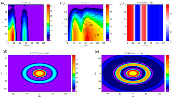
Figure 8.
The initial condition for the control experiment. (a) shows the azimuthal-mean PV (in PVU where ). (b) shows the azimuthal-mean azimuthal velocity with isosurfaces of absolute angular momentum (in units of ). (c) shows the azimuthal-mean-normalized Okubo–Weiss parameter. (d) shows the PV on , and (e) shows the potential vorticity on .
Figure 8a shows that the azimuthal-mean PV maximizes at due to the increased static stability above the surface. As shown in Figure 8d,e, the PV of this vortex exhibits a double hollow tower structure with elevated PV associated with the primary eyewall, a well-defined moat region, and a region of elevated PV associated with the secondary eyewall. The normalized Okubo–Weiss parameter shown in Figure 8c is defined as follows:
where is the relative vorticity, is the normal strain, and is the shearing strain. This parameter equals 1 when the flow is completely rotational, −1 when the flow is dominated by strain, and 0 for unidirectional shear flow. As shown in Figure 8c, the normalized Okubo–Weiss parameter is negative within the moat and outer region of the vortex and positive within the radius of maximum wind and near the secondary eyewall.
Solving Equations (8) and (9) for the parameters associated with the control experiment shows that this vortex will undergo Type-2 BI in which the most unstable mode for this vortex is with a wave growth rate of (which corresponds to an e-folding time of 0.72 h). Therefore, it is expected that there will be rapid growth in the perturbation in which there will be significant VRW growth across the moat of the vortex. The evolution of the vortex at selected times is given in Figure 9. During the first few hours of the simulation, the axisymmetric primary eyewall begins to develop a wavenumber-2 instability such that primary eyewall develops an elliptical shape. The onset of this instability leads to a rapid decay in area-integrated enstrophy and a rapid increase in area-integrated palinstrophy due to the PV mixing process. Figure 9a–d show the structure of the vortex shortly before the rapid increase in area-integrated palinstrophy. As shown in Figure 9c, the primary eyewall develops an elliptical PV structure at in the lower troposphere. However, by comparing Figure 8d with Figure 9c, it should be noted that there is minimal mixing across the primary eyewall and secondary eyewall. Furthermore, by comparing Figure 8c with Figure 9b, note that the normalized OKW parameter has decreased to small values along the outer edge of the primary eyewall and the inner edge of the secondary eyewall, which suggests that there is PV mixing across the moat of the vortex. In response to the wavenumber-2 instability, the radial flow develops a quadrupole pattern, as shown in Figure 9d. Since the formation of the elliptical eyewall starts on the outer edge of the primary eyewall, this suggests that the vortex has developed a mode of a Type-2 BI within the lower troposphere. The effect of this instability is to effectively shrink the moat width within the lower troposphere, leading to a tilted vortex, as shown in Figure 9a.
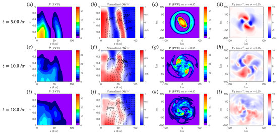
Figure 9.
The evolution of the vortex for the control experiment at (top panel), (middle panel), and (bottom panel). (a,e,i) show the azimuthal-mean PV (in PVU where ). (b,f,j) show the azimuthal-mean-normalized Okubo–Weiss parameter with isosurfaces of absolute angular momentum (in units of ). (c,g,k) show the PV on . (d,h,l) show the radial velocity on .
Figure 9e–h show the structure of the vortex when the area-integrated palinstrophy has reached its peak value after the onset of Type-2 BI. First, it should be noted that the quadrupole pattern in the radial velocity field shown in Figure 9d has largely persisted up to , as shown in Figure 9h. Since a quadrupole velocity field induces a strain pattern on the vortex, this leads to a significant reduction in the vorticity in the outer edge of the primary eyewall as low PV is mixed into the outer edge of the primary eyewall. Similarly, high PV from both eyewalls has been mixed within the moat region, producing a “PV bridge” [11] across the moat, as shown in Figure 9e,f. The evidence of this mixing can also be seen by noting that the normalized OKW parameter decreases within each eyewall (which is indicative of enhanced strain and deformation in these regions) and increases within the moat region (which is indicative of PV mixing across the moat region of the vortex), as shown in Figure 9f. It should also be noted that the PV mixing process is largely confined to the lower to mid-troposphere. This is to be expected since PV growth rates are a function of the average PV across the secondary eyewall, as shown in Equation (9).
Following the peak in area-integrated palinstrophy, the vortex approaches a monopole structure, which leads to a rapid decrease in enstrophy and palinstrophy. Figure 9h,i show the structure of the vortex as it approaches its monopole structure. By comparing Figure 9j with Figure 9f, it should be noted that PV mixing has begun to fill to moat region in the middle to upper troposphere. Furthermore, the angular momentum surfaces associated with the secondary eyewall move radially inward, and the radial flow across the vortex weakens.
The onset of Type-2 BI and the subsequent evolution of the vortex leads to a noticeable dissipation in the primary eyewall, as shown in the Hovmoller diagram in Figure 10. Notice that there is minimal change in the azimuthal wind across either eyewall during the first 5 h of vortex evolution. After the onset of Type-2 BI, the primary eyewall significantly weakens, while the secondary eyewall moves radially inward and gradually weakens. Since this numerical model does not contain a boundary layer parameterization, this indicates that the onset of Type-2 BI is connected to primary eyewall dissipation, as shown in Ref. [41]. As the primary eyewall dissipates and the secondary eyewall moves inward, the PV bridge that originally forms in the moat region becomes the eye of the new vortex, as shown in Figure 9i.
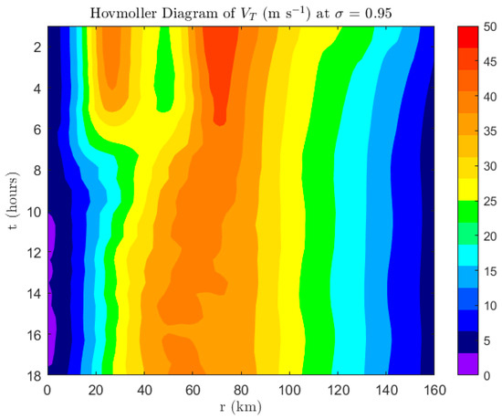
Figure 10.
The Hovmoller diagram associated with the azimuthal wind on from up to .
To assess the relative roles of mean and eddy processes in the vortex structural changes due to PV mixing, absolute angular momentum budgets were computed for the evolution of this vortex. It can be shown that the equation for azimuthally averaged absolute angular momentum in cylindrical coordinates can be written as follows:
where is the absolute angular momentum; is the azimuthal component of dissipation; and corresponds to an azimuthal average. The terms on the right-hand side of Equation (20) correspond to the radial transport of absolute angular momentum by the mean flow (RADM); the vertical transport of absolute angular momentum by the mean flow (VADM); flux divergence of angular momentum by the eddies (FLUX); the vertical transport of absolute angular momentum by eddies (VADE); the eddy azimuthal pressure gradient force (PRES); and the torque due to forcing from subgrid-scale diffusion (DISS), respectively. To show the net changes in during the onset of Type-2 BI for this vortex, Equation (20) was integrated from through (which corresponds to the time interval in which the area-integrated palinstrophy rapidly increased) using the trapezoidal rule on 15 min resolution model output.
Figure 11 shows the net changes in induced by each term in the budget. First, it should be noted that local changes in are largely concentrated within the lower troposphere for the vortex (i.e., primarily where ), consistent with the evolution shown in Figure 9. As shown in Figure 11a, the radial advection of by the mean flow (RADM) consistently acts to decrease within the lower troposphere. Since according to Figure 9, this implies that the azimuthal-mean radial velocity must be positive during this time interval. Integrating the radial velocity fields in Figure 9 from through leads to . Since the quadrupole structure of forms because of the Type-2 BI, this implies that the negative radial advection of indirectly results from the Type-2 instability.
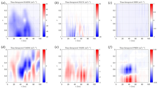
Figure 11.
The integrated budget analysis from to . The explanation for each term is found in the text.
As shown in Figure 11b, the radial advection of by the eddies (FLUX) decreases within the primary eyewall and increases within the secondary eyewall. This can be explained by noting that the Type-2 BI induces outward-propagating VRWs at the outer edge of the inner eye which mixes low-PV air from the moat region into the primary eyewall. However, the presence of positive eddy radial advection in the secondary eyewall indicates that the eddies are transporting momentum towards the secondary eyewall. For this reason, the primary eyewall rapidly dissipates (as shown in Figure 10), whereas the secondary eyewall largely maintains its strength.
Although the vertical advection terms VADM and VADE are weak compared to the radial advection terms RADM and FLUX, they both act to locally increase near the secondary eyewall in the lower troposphere, as shown in Figure 11d,e. Since according to Figure 9, this implies that , which implies weak subsidence during this time interval. The vertical motion arises based upon the structure of the radial velocity field during the onset of the Type-2 BI, as shown in Figure 9. The development of the positive vertical advection of suggests a local secondary circulation in response to the Type-2 BI within this region. Radially inward of the secondary eyewall, VADM decreases , which suggests that rising motion is decreasing in this region. Finally, we see that the eddy azimuthal pressure gradient force (PRES) and subgrid-scale diffusion (DISS) play a negligible role in the overall dynamics, as shown in Figure 11c,f.
In summary, local changes in absolute angular momentum are largely concentrated within the lower troposphere for both eyewalls. As the Type-2 BI develops, the radial advection by the mean flow and the eddies lead to inner-eyewall dissipation, whereas radial advection by the eddies transports angular momentum towards the secondary eyewall. Vertical motion develops in response to the elongation of the primary eyewall and the formation of VRWs between the primary eyewall and the moat. The PV mixing that results from Type-2 BI alters the PV across the eyewalls and the moat until the vortex approaches a monopolar state, which eliminates the Rayleigh necessary condition for BI. Thus, the mixing of PV due to Type-2 BI eventually stabilizes the vortex over time.
To further examine the role of eddy processes in the evolution of the vortex, we can examine the eddy kinetic energy budget, which allows us to understand the flow of kinetic energy between the mean flow and the eddies. Moreover, during vortex breakdown, the eddy kinetic energy corresponds to the kinetic energy associated with VRW propagation. Following Ref. [47], it can be shown that the azimuthally averaged eddy kinetic energy budget equation in cylindrical coordinates can be written as follows:
where is the eddy kinetic energy (per unit mass), , , and are the radial and azimuthal components of diffusion, respectively. The terms on the right-hand side of Equation (21) correspond to the flux divergence of by the mean flow (FDM); the flux divergence of by the eddies (FDE); the barotropic energy conversion from the mean vortex that is associated with the mean azimuthal flow (BTA); the barotropic energy conversion from the mean vortex that is associated with the mean radial flow (BTR); baroclinic energy conversion from the mean vortex associated with the mean flow (BCC); the conversion of eddy potential energy into kinetic energy (PTC); and the dissipation of eddy kinetic energy by diffusion (DISS), respectively. To show the net changes in during the onset of Type-2 BI for this vortex, Equation (21) was integrated from through (which corresponds to the time interval in which the area-integrated palinstrophy rapidly increased) using the trapezoidal rule on 15 min resolution model output.
Figure 12 shows the net changes in induced by the dominant terms in the budget analysis. First, it should be noted that the dominant source of eddy kinetic energy is the barotropic energy conversion from the mean azimuthal flow (BTA), as shown in Figure 12c. Physically, this means that the mean vortex transfers kinetic energy to the eddies through the mean azimuthal flow. In contrast, barotropic energy conversion from the mean radial flow (BTR) is a major sink for the eddy kinetic energy [as shown in Figure 12d], which means that the energy source for the radial flow shown in Figure 9 originates from the barotropic energy conversion from the eddies. Furthermore, since BTA and BTR are both major sinks of eddy kinetic energy near the secondary eyewall, this implies that VRWs transfer their kinetic energy to the mean vortex in this region, consistent with the analysis given in Figure 11. As shown in Figure 12a,b, the flux divergence of by the mean flow (FDM) and by the eddies (FDE) play a secondary role in the energy budget. However, near the primary eyewall, FDM is a source of eddy kinetic energy, indicating that the flux divergence of eddy kinetic energy from the mean vortex transports eddy kinetic energy inward from outside the primary eyewall. Conversely, FDM is a sink of eddy kinetic energy near the secondary eyewall, which suggests that the mean vortex damps eddies near the secondary eyewall.
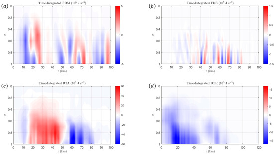
Figure 12.
The integrated budget analysis from to . See the text for the meaning for each term in the budget analysis.
In summary, it can be said that the instability of the mean azimuthal flow generates and maintains the VRWs outside of the primary eyewall, and the VRWs transfer their kinetic energy to the mean vortex in the form of radial flow. Since the azimuthally averaged radial flow is positive, this implies that VRW energy is transported towards the mean vortex near the secondary eyewall. This energy conversion process leads to a dissipation of the primary eyewall, and it provides a mechanism that helps to maintain the secondary eyewall. These considerations further confirm that the vortex breakdown is largely driven by barotropic processes.
4. Nonlinear Evolution of 3D Annular Vortices
As shown in Section 2, the most pronounced changes in linear stability are based upon changes in primary eyewall thickness , moat width , eyewall vorticity ratio , vortex hollowness , and secondary eyewall thickness . In this section, the effects of changes in , , , and on the nonlinear evolution of 3D annular vortices will be examined. Table 1 gives the parameters for the three vortices examined in this section, along with the type of BI that is expected based upon the 2D linear stability analysis given in Section 2. The azimuthal-mean PV and for each experiment are given in Figure 13. The primary eyewall vorticity for each vortex has been set such that the maximum azimuthal wind is , and the radius of the primary eyewall for each vortex has been set to .

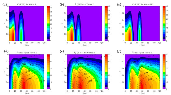
Figure 13.
The initial condition for Vortex I, II, and III. (a–c) show the azimuthal-mean PV for Vortex I, II, and III, respectively. (d–f) show the azimuthal-mean azimuthal wind with isosurfaces of absolute angular momentum (in units of ) for Vortex I, II, and III, respectively.
4.1. Results from Vortex I
In comparison with the control experiment, the primary eyewall thickness parameter has increased from to for Vortex I, which implies a thinner primary eyewall. According to the linear analysis of Section 2, an increase in (i.e., thinning the primary eyewall) within this parameter space causes an overlap between Type-2 BI across the moat and Type-3 BI across the primary eyewall. However, the fastest growing mode is associated with the Type-3 BI. The evolution of Vortex I at selected times is shown in Figure 14. During the first few hours of the simulation, the primary eyewall begins to develop a polygonal shape, and similar to the control experiment, the onset of BI leads to an increase in area-integrated palinstrophy. Figure 14a–d show the structure of the vortex shortly before the increase in area-integrated palinstrophy. Unlike the control experiment, there is minimal PV mixing within the moat region [as shown by the negligible changes in normalized OKW in Figure 14b], which indicates that Type-2 BI has not occurred. However, there is PV mixing between the primary eyewall and the vortex center, which signals the onset of Type-3 BI. Unlike the Type-2 BI shown in the control experiment, it should be noted that the primary eyewall strength remains approximately constant during the onset of Type-3 BI.
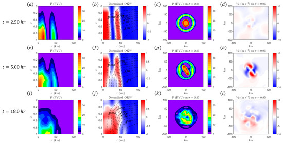
Figure 14.
The evolution of the vortex for Vortex I at (top panel), (middle panel), and (bottom panel). (a,e,i) show the azimuthal-mean PV (in PVU where ). (b,f,j) show the azimuthal-mean-normalized Okubo–Weiss parameter with isosurfaces of absolute angular momentum (in units of ). (c,g,k) show the PV on . (d,h,l) show the radial velocity on .
In response to the onset of Type-3BI, the primary eyewall develops a wavenumber-4 structure, which indicates that VRWs have formed in this region. However, as the vortex continues to evolve, the dominant mode of BI shifts from Type-3 to Type-2, as the effective moat width decreases during the initial mixing process. Figure 14e–h show the structure of the vortex shortly before the rapid increase in area-integrated palinstrophy associated with Type-2 BI. Notice that the primary eyewall develops an elliptical shape [as shown in Figure 14g] with a quadrupole radial velocity structure [as shown in Figure 14h]. Moreover, notice that there is significant mixing across the moat, as shown in Figure 14f, consistent with the Type-2 BI discussed in the control experiment. After the onset of Type-2 BI, Vortex I evolves in a manner similar to the control experiment. Figure 14h,i show the structure of Vortex I as it approaches its monopole structure. By comparing Figure 14e with Figure 14i, notice that the primary eyewall dissipates and that the secondary eyewall moves radially inward.
The differences between the Type-2 and Type-3 BI can be seen by analyzing their respective effects on the angular momentum budget, which is shown in Figure 15. As shown in Section 3, the dominant terms in the angular momentum budget are the radial advection of due to the mean flow (RADM) and due to the eddies (FLUX). During the onset of Type-3 BI, FLUX acts to increase in the vicinity of the primary eyewall [as shown in Figure 15b], whereas it has negligible influence outside of the eyewall. Furthermore, by comparing Figure 15a and Figure 15b in the lower troposphere, the FLUX term partially balances the RADM term near the primary eyewall, which helps to explain why there is minimal change in the absolute angular momentum during the onset of Type-3 BI. In contrast, the onset of Type-2 BI leads to a significant growth in the radial advection of by the mean flow on the outer edge of the primary eyewall. Even though the FLUX term also increases during the onset of Type-2 BI, its magnitude is less than the magnitude of the RADM term, which explains why primary eyewall dissipation begins after the onset of PV mixing between the primary eyewall and the moat.
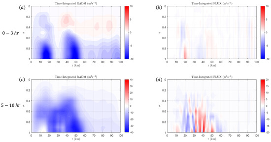
Figure 15.
The integrated budget analysis from to (top panel) and from to (bottom panel) for Vortex I. The top panel corresponds to the time interval in which Type-3 BI is the dominant instability, whereas the bottom panel corresponds to the time interval in which Type-2 BI is the dominant instability. See the text for the meaning of each term in the budget analysis.
Similar conclusions can be drawn by examining the eddy kinetic energy budget, as shown in Figure 16. As shown in Section 3, the dominant terms in the eddy kinetic energy budget are the flux divergence of by the mean flow (FDM), the barotropic energy conversion from the mean azimuthal flow (BTA), and the barotropic energy conversion from the mean radial flow (BTR). As shown in Figure 16a–c, the instability in the azimuthal flow through the BTA term transfers kinetic energy from the mean flow near the primary eyewall to the eddies, and the radial flow associated with Type-3 BI arises from the eddies through the BTR term. During the transition to Type-2 BI, the source of eddy kinetic energy arises from the azimuthal flow within the moat region, as shown in Figure 16e. However, since the BTA and BTR terms are sinks of eddy kinetic energy near the secondary eyewall, this implies that eddies (in the form of VRWs) are transporting their kinetic energy to the mean vortex. The combination of these effects leads to a weakening of the primary eyewall and a maintenance of the secondary eyewall, similar to the control experiment.

Figure 16.
The integrated budget analysis from to (top panel) and from to (bottom panel) for Vortex I. The top panel corresponds to the time interval in which Type-3 BI is the dominant instability, whereas the bottom panel corresponds to the time interval in which Type-2 BI is the dominant instability. See the text for the meaning of each term in the budget analysis.
4.2. Results from Vortex II
In comparison with the control experiment, the moat width parameter has increased from to , which implies a smaller moat between the eyewalls. According to the linear stability analysis of Section 2, it is expected that this vortex will undergo Type-2 BI with a most unstable mode of . The evolution of Vortex II at selected times is shown in Figure 17. During the first few hours of the model simulation, PV mixing occurs across the moat region (which is consistent with Type-2 BI); however, the primary eyewall develops a tripole structure rather than an elliptical structure. Figure 17a–d show the structure of the vortex shortly before the rapid increase in palinstrophy associated with Type-2 BI. Note that the moat region develops a tripole structure in the PV field [as shown in Figure 17c] and that the tripole PV structure is accompanied by a hexapole structure in the radial velocity field, as shown in Figure 17d. The tripole structure associated with the Type-2 BI is due to the presence of counter-propagating VRWs, and these VRWs propagate cyclonically around the vortex where divergence is found downstream of the wave axis and convergence is found upstream of the wave axis. Figure 17e–h show the structure of the vortex after the VRWs rotate one-quarter wavelength around the vortex. During the axisymmetrization process, there is significant mixing in the moat region within the lower troposphere [as shown by comparing Figure 17a with Figure 17e] and the VRWs propagate outward from the moat region. Consequently, Vortex II reaches its monopole state faster than the control experiment. By comparing the evolution of the control experiment to Vortex I, we see that the timescale for primary eyewall dissipation decreases as the moat width decreases. Conversely, it is expected that a larger moat region between the eyewalls can stabilize a 3D annular vortex, as discussed in Section 2.
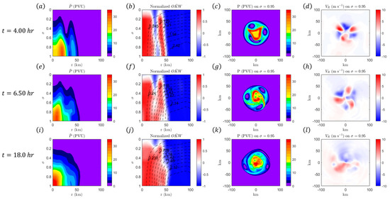
Figure 17.
The evolution of the vortex for Vortex II at (top panel), (middle panel), and (bottom panel). (a,e,i) show the azimuthal-mean PV (in PVU where ). (b,f,j) show the azimuthal-mean-normalized Okubo–Weiss parameter with isosurfaces of absolute angular momentum (in units of ). (c,g,k) show the PV on . (d,h,l) show the radial velocity on .
The differences in vortex evolution for Vortex II and the control experiment can be investigated by examining the absolute angular momentum and eddy kinetic energy budget, which is shown in Figure 18. By comparing Figure 18a with Figure 11a, we see that the RADM term is larger in magnitude for Vortex I than the control experiment near the primary eyewall. This is primarily based upon a larger azimuthal-mean radial outflow for Vortex II. In contrast, by comparing Figure 18b with Figure 11b, the FLUX term is smaller in magnitude and more radially constrained for Vortex I than the control experiment near the primary eyewall. This can be explained by noting that the stagnation radius for VRWs varies inversely with the azimuthal wavenumber [48]. Therefore, the wave energy associated with VRWs from the outer edge of the primary eyewall accumulates at a smaller radius. However, since the moat region is smaller for Vortex II, PV can be efficiently mixed within the moat region to the inner edge of the secondary eyewall.
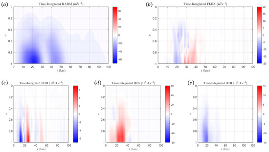
Figure 18.
The integrated budget analysis (top panel) and the integrated budget analysis (bottom panel) from to for Vortex I. See the text for the meaning of each term in the budget analysis.
Similarly, by comparing Figure 18c–e with Figure 12, we see that the dominant terms in the eddy kinetic energy budget are more radially constrained for Vortex II than for the control experiment. In particular, the BTA term (which is the source of VRW energy from the mean vortex) and the BTR term (which is the energy source for radial flow during the onset of Type-2 BI) are strongly confined near the outer edge of the primary eyewall. Therefore, it can be said that the instability within the azimuthal flow generates wavenumber-3 VRWs, and their energy generates radial flow near the primary eyewall with a tripole structure. During the axisymmetrization process, the VRW energy accumulates at a smaller radius than the control experiment.
4.3. Results from Vortex III
In comparison with the control experiment, the eyewall vorticity ratio parameter has decreased from to , and the secondary eyewall thickness parameter has increased from to . Thus, Vortex III has a stronger, thinner secondary eyewall than the control experiment. According to the linear analysis of Section 2, these changes within this parameter space cause an overlap between Type-1 BI across the secondary eyewall and Type-2 BI across the moat. The evolution of Vortex III at selected times is shown in Figure 18. During the first three hours of the model simulation, an instability develops across the secondary eyewall, producing a collection of mesovortices. Since this instability leads to no appreciable mixing across the moat or across the primary eyewall, this corresponds to Type-1 BI. Figure 19a–d display the state of the vortex shortly before the increase in area-integrated palinstrophy associated with Type-1 BI. As shown in Figure 19c, a collection of 12 mesovortices develops across the secondary eyewall, consistent with the linear stability analysis from Section 2. These mesovortices arise from VRWs across the secondary eyewall which generate substantial strain and deformation [as shown in Figure 19c] and regions of alternating radial inflow and outflow across the secondary eyewall [as shown in Figure 19d].
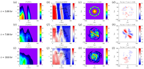
Figure 19.
The evolution of the vortex for Vortex III at (top panel), (middle panel), and (bottom panel). (a,e,i) show the azimuthal-mean PV (in PVU where ). (b,f,j) show the azimuthal-mean-normalized Okubo–Weiss parameter with isosurfaces of absolute angular momentum (in units of ). (c,g,k) show the PV on . (d,h,l) show the radial velocity on .
The onset of Type-1 BI across the secondary eyewall increases the effective thickness of the secondary eyewall and reduces the azimuthal-mean PV of the secondary eyewall over time, which permits the development of Type-2 BI across the moat. Figure 19e–h show the state of the vortex at the peak of the area-integrated palinstrophy associated with Type-2 BI. Notice that the radial velocity field develops a quadrupole structure just as in the control experiment, but the strength of the radial outflow regions across the moat has increased, as shown in Figure 19h. This implies that there is a significant transfer of eddy kinetic energy to the mean vortex, which will be shown below. By comparing Figure 19f to Figure 9f, we see that there is much more deformation and strain present during the axisymmetrization process for Vortex III than the control experiment. For this reason, the dissipation of the primary eyewall occurs rapidly during the onset of Type-2 BI. Figure 19i–l show the state of the vortex as it approaches a vortex monopole. By comparing Figure 19a with Figure 19i, we see that the primary eyewall has rapidly dissipated, while the secondary eyewall moved radially inwards in response to Type-2 BI.
The differences between the Type-1 and Type-2 BI can be seen by analyzing their respective effects on the angular momentum budget, which is shown in Figure 20. During the onset of Type-1 BI, the FLUX term acts to increase in the vicinity of the secondary eyewall [as shown in Figure 20b], whereas the RADM term acts to decrease in the vicinity of the eyewall [as shown in Figure 20a]. Furthermore, since the VRWs have a high azimuthal wavenumber (where ), VRW energy has a relatively small propagation distance. For this reason, the radial extent of both terms is small around the secondary eyewall. For Vortex III, the onset of Type-2 BI leads to strong flux divergence of within the moat region, as shown in Figure 20d. This helps to explain the significant mixing (and increased absolute angular momentum) that occurs near in Figure 19e–g. Outside of this region, the RADM term acts to decrease , especially within the primary eyewall, as shown in Figure 20c. As mentioned in Section 3.2, positive axisymmetric radial advection in the angular momentum budget is associated with positive azimuthal-mean radial flow, which is consistent with the radial velocity field shown in Figure 19h. In summary, it can be said that the Type-1 BI leads to significant PV mixing in the region surrounding the secondary eyewall (which effectively weakens ), and this PV mixing sets the stage for the Type-2 BI between the moat and the primary eyewall.
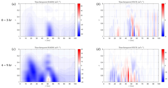
Figure 20.
The integrated budget analysis from to (top panel) and from to (bottom panel) for Vortex I. The top panel corresponds to the time interval in which Type-1 BI is the dominant instability, whereas the bottom panel corresponds to the time interval in which Type-2 BI is the dominant instability. See the text for the meaning of each term in the budget analysis.
The eddy kinetic energy budget, as shown in Figure 21, can be used to further explain the rapid changes in Vortex III compared to the control experiment. The development of the Type-1 BI is evidenced by the barotropic conversion of kinetic energy from the azimuthal flow near the secondary eyewall, as shown in Figure 21b. Notice that the FDM and BTA terms have opposite signs near , as shown in Figure 21a, which implies that the eddies obtain their energy from the flow instability and the eddies are damped by the shearing flow. Furthermore, the eddies transfer some of their energy to the mean vortex in the form of radial flow, as shown in the radial velocity field given in Figure 19d. During the transition to Type-2 instability, the magnitude of the BTA term for Vortex III [as shown in Figure 21d] is approximately 30% larger than the magnitude of the BTA term for the control experiment [as shown in Figure 12c]. This helps to explain the rapid growth of VRWs in the moat region and the rapid dissipation of the primary eyewall for Vortex III. Furthermore, the enhanced magnitude of the BTR term for Vortex III compared to the control experiment helps to explain the pronounced radial velocity field shown in Figure 19h.
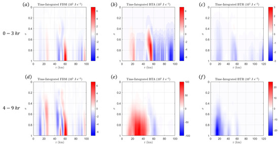
Figure 21.
The integrated budget analysis from to (top panel) and from to (bottom panel) for Vortex III. The top panel corresponds to the time interval in which Type-3 BI is the dominant instability, whereas the bottom panel corresponds to the time interval in which Type-2 BI is the dominant instability. See the text for the meaning of each term in the budget analysis.
5. Discussions and Conclusions
In this manuscript, the stability and evolution of annular vortices with a double-eyewall structure were examined. By performing a linear stability analysis on 2D annular vortices with a double-eyewall structure, as shown in Figure 1, it was shown that the stability of these vortices depends upon eight dimensionless parameters: (1) the hollowness of the vortex , (2) the eyewall vorticity ratio , (3) the moat strength , (4) the skirt strength , (5) the primary eyewall thickness , (6) the moat width , (7) the secondary eyewall thickness , and the skirt width .
In addition, it was shown the type of BI that develops for these types of vortices depends principally upon , , , , and . The parameter range in which the vortex is stable is , , , and , which physically corresponds to annular vortices with a thick primary eyewall, a thick secondary eyewall, and a large moat. The parameter range in which Type-1 BI is excited across the secondary eyewall is , , , and , which physically corresponds to annular vortices with a thick primary eyewall, a large moat, and a strong, thin secondary eyewall. The parameter range in which Type-2 BI is excited across the moat of vortex is , , and , which physically corresponds to annular vortices with a small moat and a relatively weak secondary eyewall. Finally, the parameter range in which Type-3 BI is excited across the primary eyewall is , , , , and , which physically corresponds to annular vortices with a thin, strong primary eyewall, a large moat, and a weak secondary eyewall.
The 2D linear stability analysis indicates that Type-2 BI has the least restrictive parameter range, where Type-2 BI can be excited even for thin secondary eyewalls and/or thin primary eyewalls if the moat width is sufficiently small (i.e., ). For this reason, the most common type of BI for annular vortices with a double-eyewall structure is Type-2 BI. Conversely, Type-3 BI has the most restrictive parameter range since the presence of a strong, central vortex (i.e., large ) or the presence of a sufficiently strong secondary eyewall (i.e., ) can eliminate the presence of Type-3 BI.
The theoretical framework from the 2D linear stability analysis was used to interpret the nonlinear evolution of 3D annular vortices with a double-eyewall structure. For a 3D vortex undergoing Type-2 BI, it was shown that the primary eyewall develops an elliptical structure in which the radial velocity field develops a quadrupole structure. Absolute angular momentum budget analysis indicates that during the onset of Type-2 BI, azimuthally averaged radial outflow occurs across the moat (which leads to a rapid decrease in the intensity of the primary eyewall), and the eddies transport absolute angular momentum radially outward towards the secondary eyewall (which helps to maintain the intensity of the secondary eyewall). Eddy kinetic energy budget analysis indicates that the instability associated with the azimuthal flow in the primary eyewall is the energy source of the eddies, while the eddies themselves transfer energy to the mean vortex in the form of radial flow during the axisymmetrization process of the vortex. As PV is mixed between the moat and the primary eyewall, the moat vorticity gradually increases, which stabilizes the vortex to Type-2 BI according to the linear stability analysis. Eventually, the vortex approaches its end state as a monopole in which the secondary eyewall replaces the primary eyewall. This process indicates that the onset of Type-2 BI aids in the dissipation of the primary eyewall during an ERC, as suggested in [41].
The effects of changes in , , , and on the nonlinear evolution of 3D annular vortices were examined. The 2D linear stability analysis indicated that an increase in (i.e., thinning of the primary eyewall) shifts the Type-2 BI towards a Type-3 BI (i.e., BI across the primary eyewall). The 3D model simulation shows that the onset of Type-3 BI produces a polygonal eyewall structure, which indicates that counter-propagating VRWs have formed in this region [3]. Since the VRWs associated with Type-3 BI can have a high azimuthal wavenumber, this implies that the wave energy is largely confined to the primary eyewall and the outer eye region. However, the VRWs mix PV and angular momentum between the primary eyewall and the eye of the vortex. This process increases the hollowness of the vortex, which stabilizes the vortex to Type-3 BI (as shown in Ref. [40]) and allows Type-2 BI to ensue. The difference in the eddy kinetic energy transfer between Type-2 and Type-3 BI is connected to the substantial difference in PV mixing between these types of instabilities, as suggested by [49].
Second, it was shown (via the 2D linear stability analysis) that an increase in (i.e., decrease in the moat width) shifts the most unstable mode of the Type-2 BI towards higher azimuthal wavenumber numbers with large wave growth rates. The 3D model simulation shows that the timescale for axisymmetrization (and the accompanying primary eyewall dissipation) is reduced as the moat width decreases. This is consistent with the hypothesis from Ref. [50] which speculated that BI plays a role in determining the maintenance time of the double-eyewall structures. As the moat width decreases, VRWs with a higher azimuthal wavenumber propagate across the moat of the vortex, and since the stagnation radius of VRWs is inversely related to the azimuthal wavenumber, VRW energy is strongly sheared just outside of the vortex.
Third, it was shown (via the 2D linear stability analysis) that an increase in (i.e., thinning of the secondary eyewall) shifts the Type-2 BI towards a Type-1 BI (i.e., BI across the secondary eyewall) only when . The 3D model simulation shows that the onset of Type-1 BI produces mesovortices and counter-propagating VRWs across the secondary eyewall. Since thin secondary eyewalls generate VRWs with a high azimuthal wavenumber, wave energy is strongly confined to the near region between the secondary eyewall and the moat. As the VRWs mix PV within this region, the effective moat vorticity increases, which stabilizes the vortex to Type-1 BI, as shown in the linear stability analysis in Section 2. In general, the axisymmetrization process associated with the Type-1 BI or Type-3 BI can rearrange the PV within the annular vortex, which sets the stage for Type-2 BI to occur if the moat width is sufficiently small.
The analysis in this paper can be used to explain how BI aids in the evolution of eyewall replacement cycles (ERCs). As discussed in Ref. [39], the evolution of an ERC occurs in three phases: (1) Stage I corresponds to an intensification phase where the primary eyewall reaches its maximum intensity and the secondary eyewall has formed, (2) Stage II corresponds to the weakening phase in which the primary eyewall weakens while the secondary eyewall contracts and intensifies, and (3) Stage III corresponds to the re-intensification phase in which the secondary eyewall becomes stronger than the primary eyewall and fully replaces the primary eyewall. During Stage I, the TC vortex becomes a 3D annular vortex with a double-eyewall structure, which implies that it is susceptible to BI. As the secondary eyewall continues to intensify, the eyewall vorticity ratio decreases, and as the secondary eyewall contracts, the moat width decreases. As the 2D linear stability analysis in Figure 5 shows, the conditions for Type-1 and Type-2 BI may both be present in the vortex. Since convection will continuously generate PV across the secondary eyewall, this implies that the dominant instability will be Type-2 BI. The onset of Type-2 BI begins Stage II in which the primary eyewall dissipates (based upon PV mixing and radial outflow within the moat region). Although convection helps to maintain the strength of the secondary eyewall, the outward-directed momentum flux from the VRWs helps to maintain the strength of the secondary eyewall [51].
In closing, this manuscript focused upon the adiabatic evolution of 3D annular vortices. First, it should be noted that the impacts of convection (and the accompanying secondary circulation) have been neglected in this study. As shown in Ref. [22], convection will directly impact the eyewall vorticity ratio , the primary eyewall thickness , and the secondary eyewall thickness as the vortex evolves over time. Furthermore, the presence of the secondary circulation will produce changes in the eddy kinetic energy and absolute angular momentum budgets as baroclinic processes begin to play an important role in the evolution of these vortices. Second, the impacts of vertical structure (i.e., the baroclinity of the base-state) have also been neglected in this study. Although the budget analyses of this work have shown that vertical advective processes play a minor role in the adiabatic evolution of these vortices, previous work [48] has shown that excited VRWs can propagate vertically, and they can have behavior that differs substantially from the barotropic evolution given in this study. Further investigations are required to further understand these subjects.
Funding
This research received no external funding.
Data Availability Statement
The original contributions presented in this study are included in this article. Further inquiries can be directed to the corresponding author.
Acknowledgments
The calculations were made on Linux workstations generously provided by The Citadel. The funding for this work comes from The Citadel. I would also like to thank the two anonymous reviewers for their penetrating and honest reviews, which substantially improved the quality of this paper.
Conflicts of Interest
The author declares no conflicts of interest.
Appendix A. The Matrix
As shown in Section 2, the dominant wave growth rate for the linear stability analysis is determined by solving Equation (8) for the matrix . Since is a matrix, it has the following form:
where each matrix element is given below in which and .
References
- Willoughby, H.E.; Clos, J.A.; Shoreibah, M.G. Concentric eyewalls, secondary wind maxima, and the evolution of the hurricane vortex. J. Atmos. Sci. 1982, 39, 395–411. [Google Scholar] [CrossRef]
- Montgomery, M.T.; Kallenbach, R.J. A theory for vortex Rossby waves and its application to spiral bands and intensity changes in hurricanes. Q. J. R. Meteorol. Soc. 1997, 123, 435–465. [Google Scholar] [CrossRef]
- Schubert, W.H.; Montgomery, M.T.; Taft, R.K.; Guinn, T.A.; Fulton, S.R.; Kossin, J.P.; Edwards, J.P. Polygonal eyewalls, asymmetric eye contraction, and potential vorticity mixing in hurricanes. J. Atmos. Sci. 1999, 56, 1197–1223. [Google Scholar] [CrossRef]
- Hendricks, E.A.; Montgomery, M.T.; Davis, C.A. The role of “vortical” hot towers in the formation of Tropical Cyclone Diana (1984). J. Atmos. Sci. 2004, 61, 1209–1232. [Google Scholar] [CrossRef]
- Montgomery, M.T.; Nicholls, M.E.; Cram, T.A.; Saunders, A.B. A vortical hot tower route to tropical cyclogenesis. J. Atmos. Sci. 2006, 63, 355–386. [Google Scholar] [CrossRef]
- Hausmann, S.A.; Ooyama, K.V.; Schubert, W.H. Potential vorticity structure of simulated hurricanes. J. Atmos. Sci. 2006, 63, 87–108. [Google Scholar] [CrossRef]
- Martinez, J.; Bell, M.M.; Rogers, R.F.; Doyle, J.D. Axisymmetric potential vorticity evolution of Hurricane Patricia (2015). J. Atmos. Sci. 2019, 76, 2043–2063. [Google Scholar] [CrossRef]
- Eliassen, A. The Charney-Stern theorem on barotropic-baroclinic instability. Pure Appl. Geophys. 1983, 121, 563–572. [Google Scholar] [CrossRef]
- Montgomery, M.T.; Shapiro, L.J. Generalized Charney-Stern and Fjortoft theorems for rapidly rotating vortices. J. Atmos. Sci. 1995, 52, 1829–1833. [Google Scholar] [CrossRef]
- Hendricks, E.A.; Schubert, W.H.; Taft, R.K.; Wang, H.; Kossin, J.P. Lifecycles of hurricane-like vorticity rings. J. Atmos. Sci. 2009, 66, 705–722. [Google Scholar] [CrossRef]
- Hendricks, E.A.; Schubert, W.H. Adiabatic rearrangement of hollow PV towers. J. Adv. Model. Earth Syst. 2010, 2, 1–19. [Google Scholar] [CrossRef]
- Hendricks, E.A.; Schubert, W.H.; Chen, Y.-H.; Kuo, H.-C. Hurricane eyewall evolution in a forced shallow-water model. J. Atmos. Sci. 2014, 71, 1623–1643. [Google Scholar] [CrossRef]
- Kossin, J.P.; Schubert, W.H. Mesovortices, polygonal flow patterns, and rapid pressure falls in hurricane-like vortices. J. Atmos. Sci. 2011, 58, 2196–2209. [Google Scholar] [CrossRef]
- Kwon, Y.; Frank, W.M. Dynamic instabilities of simulated hurricane-like vortices and their impacts on the core structure of hurricanes. Part I: Dry experiments. J. Atmos. Sci. 2005, 62, 3955–3973. [Google Scholar] [CrossRef]
- Menelaou, K.; Yau, M.K.; Martinez, Y. Impact of asymmetric dynamical processes on the structure and intensity change of two-dimensional hurricane-like annular vortices. J. Atmos. Sci. 2013, 70, 559–582. [Google Scholar] [CrossRef]
- Menelaou, K.; Yau, M.K.; Martinez, Y. On the origin and impact of a polygonal eyewall in the rapid intensification of Hurricane Wilma. J. Atmos. Sci. 2013, 70, 3839–3858. [Google Scholar] [CrossRef]
- Nolan, D.S.; Montgomery, M.T. The algebraic growth of wavenumber one disturbances in hurricane-like vortices. J. Atmos. Sci. 2000, 57, 3514–3538. [Google Scholar] [CrossRef]
- Nolan, D.S.; Montgomery, M.T. Nonhydrostatic, three-dimensional perturbations to balanced, hurricane-like vortices. Part I: Linearized formulation, stability, and evolution. J. Atmos. Sci. 2002, 59, 2989–3020. [Google Scholar] [CrossRef]
- Rozoff, C.M.; Schubert, W.H.; McNoldy, B.D.; Kossin, J.P. Rapid filamentation zones in intense tropical cyclones. J. Atmos. Sci. 2006, 66, 133–147. [Google Scholar] [CrossRef]
- Rozoff, C.M.; Kossin, J.P.; Schubert, W.H.; Mulero, P.J. Internal control of hurricane intensity: The dual nature of potential vorticity mixing. J. Atmos. Sci. 2009, 66, 133–147. [Google Scholar] [CrossRef]
- Terway, W.D.; Montgomery, M.T. Wavenumber-2 and wavenumber-m vortex Rossby wave instabilities in a generalized three-region model. J. Atmos. Sci. 2002, 59, 2421–2427. [Google Scholar] [CrossRef]
- Williams, G.J. The generation and maintenance of hollow PV towers in a forced primitive equation model. Meteorol. Atmos. Phys. 2019, 131, 1635–1659. [Google Scholar] [CrossRef]
- Chen, Y.; Yau, M.K. Spiral bands in a simulated hurricane. Part I: Vortex Rossby wave verification. J. Atmos. Sci. 2001, 58, 2128–2145. [Google Scholar] [CrossRef]
- Kwon, Y.; Frank, W.M. Dynamical instabilities of simulated hurricane-like vortices and their impacts on the core structure of hurricanes. Part II: Moist experiments. J. Atmos. Sci. 2008, 65, 106–122. [Google Scholar] [CrossRef]
- Nguyen, C.M.; Reeder, M.J.; Davidson, N.E.; Smith, R.K.; Montgomery, M.T. Inner-core vacillation cycles during the intensification of Hurricane Katrina. Q. J. R. Meteorol. Soc. 2011, 137, 829–844. [Google Scholar] [CrossRef]
- Wu, C.-C.; Cheng, H.-J.; Wang, Y.; Chou, K.-H. A numerical investigation of the eyewall evolution of a landfalling typhoon. Mon. Weather Rev. 2009, 137, 21–40. [Google Scholar] [CrossRef]
- Wu, C.-C.; Wu, S.-N.; Wei, H.-H.; Abarca, S.F. The role of convective heating in tropical cyclone eyewall ring evolution. J. Atmos. Sci. 2016, 73, 319–330. [Google Scholar] [CrossRef]
- Yang, B.; Yang, Y.; Wang, B. The effect of internally generated inner-core asymmetries on tropical cyclone potential intensity. J. Atmos. Sci. 2007, 64, 1165–1188. [Google Scholar] [CrossRef]
- Yau, M.K.; Liu, Y.; Zhang, D.-L.; Chen, Y. A multiscale numerical study of Hurricane Andrew (1992). Part VI: Small-scale inner-core structures and wind streaks. Mon. Weather Rev. 2004, 132, 1410–1433. [Google Scholar] [CrossRef]
- Hendricks, E.A.; McNoldy, B.D.; Schubert, W.H. Observed inner-core structural variability in Hurricane Dolly (2008). Mon. Weather Rev. 2012, 140, 4066–4077. [Google Scholar] [CrossRef]
- Kossin, J.P.; Eastin, M.D. Two distinct regimes in the kinematic and thermodynamic structure of the hurricane eye and eyewall. J. Atmos. Sci. 2001, 58, 1079–1090. [Google Scholar] [CrossRef]
- Kossin, J.P.; McNoldy, B.D.; Schubert, W.H. Vortical swirls in hurricane eye clouds. Mon. Weather Rev. 2002, 130, 3144–3149. [Google Scholar] [CrossRef]
- Kossin, J.P.; Schubert, W.H. Mesovortices in Hurricane Isabel. Bull. Am. Meteorol. Soc. 2004, 85, 151–153. [Google Scholar] [CrossRef]
- Montgomery, M.T.; Vladimirov, V.A.; Denissenko, P.V. An experimental study on hurricane mesovortices. J. Fluid Mech. 2002, 471, 1–32. [Google Scholar] [CrossRef]
- Reasor, P.D.; Montgomery, M.T.; Marks, F.D.; Gamache, J.F. Low-wavenumber structure and evolution of the hurricane inner core observed by airborne dual-Doppler radar. Mon. Weather Rev. 2000, 128, 1653–1680. [Google Scholar] [CrossRef]
- Kossin, J.P.; Sitkowski, M. An objective model for identifying secondary eyewall formation in hurricane. Mon. Weather Rev. 2009, 137, 876–892. [Google Scholar] [CrossRef]
- Samsury, C.E.; Zipser, E.J. Secondary wind maxima in hurricanes: Airflow and relationship to rainbands. Mon. Weather Rev. 1995, 123, 3502–3517. [Google Scholar] [CrossRef][Green Version]
- Houze, R.A.; Chen, S.S.; Smull, B.F.; Lee, W.-C.; Bell, M.M. Hurricane intensity and eyewall replacement. Science 2007, 315, 1235–1239. [Google Scholar] [CrossRef]
- Sitkowski, M.; Kossin, J.P.; Rozoff, C.M. Intensity and structure changes during hurricane eyewall replacement cycles. Mon. Weather Rev. 2011, 139, 3829–3847. [Google Scholar] [CrossRef]
- Kossin, J.P.; Schubert, W.H.; Montgomery, M.T. Unstable interactions between a hurricane’s primary eyewall and a secondary ring of enhanced vorticity. J. Atmos. Sci. 2000, 57, 3893–3917. [Google Scholar] [CrossRef]
- Lai, T.-K.; Menelaou, K.; Yau, M.K. Barotropic instability across the moat and primary eyewall dissipation: A numerical study of Hurricane Wilma (2005). J. Atmos. Sci. 2019, 76, 989–1013. [Google Scholar] [CrossRef]
- Rostami, M.; Zeitlin, V. Evolution of double-eyewall hurricanes and emergence of complex tripolar end states in moist-convective rotating shallow water model. Phys. Fluids 2022, 34, 3–16. [Google Scholar] [CrossRef]
- Schecter, D.A.; Montgomery, M.T. On the symmetrization rate of an intense geophysical vortex. Dyn. Atmos. Ocean. 2003, 37, 55–88. [Google Scholar] [CrossRef]
- Hendricks, E.A. Tropical Cyclone Evolution via Internal Asymmetric Dynamics. Ph.D. Thesis, Colorado State University, Fort Collins, CO, USA, 2008. [Google Scholar]
- Wang, Y. An explicit simulation of tropical cyclones with a triply nested movable mesh primitive equation model: TCM3. Part I: Model description and control experiment. Mon. Weather Rev. 2001, 129, 1370–1394. [Google Scholar] [CrossRef]
- Dunion, J.P.; Marron, C.S. A reexamination of the Jordan mean tropical sounding based on awareness of the Saharan air layer: Results from 2002. J. Clim. 2008, 21, 5242–5253. [Google Scholar] [CrossRef]
- Wang, Y. Vortex Rossby waves in a numerically simulated tropical cyclone. Part I: Overall structure, potential vorticity, and kinetic energy budgets. J. Atmos. Sci. 2002, 59, 1213–1238. [Google Scholar] [CrossRef]
- Gao, C.; Zhu, P. Vortex Rossby wave propagation in baroclinic tropical cyclone-like vortices. Geophys. Res. Lett. 2016, 43, 12578–12589. [Google Scholar] [CrossRef]
- Slocum, C.J.; Taft, R.K.; Kossin, J.P.; Schubert, W.H. Barotropic instability during eyewall replacement. Meteorology 2023, 2, 191–221. [Google Scholar] [CrossRef]
- Yang, Y.-T.; Kuo, H.-C.; Hendricks, E.A.; Peng, M.S. Structural and intensity changes of concentric eyewall typhoons in the western North Pacific basin. Mon. Weather Rev. 2013, 141, 2632–2648. [Google Scholar] [CrossRef]
- Lai, T.-K.; Hendricks, E.A.; Yau, M.K.; Menelaou, K. Roles of barotropic instability across the moat in the primary eyewall decay and secondary eyewall intensification: Essential dynamics. J. Atmos. Sci. 2021, 78, 1411–1428. [Google Scholar] [CrossRef]


Disclaimer/Publisher’s Note: The statements, opinions and data contained in all publications are solely those of the individual author(s) and contributor(s) and not of MDPI and/or the editor(s). MDPI and/or the editor(s) disclaim responsibility for any injury to people or property resulting from any ideas, methods, instructions or products referred to in the content. |
© 2024 by the author. Licensee MDPI, Basel, Switzerland. This article is an open access article distributed under the terms and conditions of the Creative Commons Attribution (CC BY) license (https://creativecommons.org/licenses/by/4.0/).