1. Introduction
In recent years, the fifth generation of communication networks, or simply 5G, has been continuously reshaping the ICT landscape. Along with the advent of 5G and beyond technologies, many services have also emerged, including augmented and virtual reality, vehicle-to-everything communications, e-health, and smart homes. Due to this diversity of existing services, the International Telecommunication Union (ITU) has identified three major usage scenarios for 5G services, namely: Ultra-Reliable Low Latency Communications (uRLLC), Enhanced Mobile Broadband (eMBB), and Massive Machine Type Communications (mMTC) [
1]. Each of these usage scenarios has specific requirements that distinguish the types of resources allocated for each service request. To be specific, adaptive and on-demand resource provisioning methods based on varying service request types are needed to meet user needs [
2]. Moreover, it is essential to meet the various requirements of these services to provide end-users with the best quality of service (QoS) possible.
One of the critical technologies on 5G and beyond systems is network slicing (NS) [
3]. NS refers to creating multiple virtual networks within a 5G physical infrastructure to constitute a physical network. This technology is made possible by Software-Defined Networking (SDN) [
4] and Network Function Virtualization (NFV) [
5]. Moreover, each slice in the network has certain network functions tailored to the different services required by users. A classification of these slices includes service, resource, and deployment-driven NS solutions [
6]. Moreover, creating slices for specific services within the physical network also ensures that network resources are efficiently utilized or allocated throughout the system. Likewise, NScan be broken down into three major processes: slice creation, slice isolation, and slice management [
7]. This categorization of NS processes is further expanded into slice monitoring, slice mapping, and slice provisioning, as discussed in [
8].
Recently, NS has become the subject of most research related to 5G networks, as it can improve service delivery and QoS. For example, the work in [
9] studied the management and allocation of radio access networks (RAN) resources focusing on its impact on uRLLC and eMBB slices. The authors proposed an intelligent decision-making technique to manage network traffic and allocate the required resources. The work in [
10] enumerates several factors that affect the implementation of network slices. These include resource allocation, slice isolation, security, RAN virtualization, feature granularity, and end-to-end (E2E) slice orchestration. Sohaib et al. presented the applications of machine learning (ML) and artificial intelligence (AI) for NS solutions in [
11]. Their paper listed various ML and AI algorithms, and applications for different NS use-cases such as mobility prediction and resource management. Reference [
12] studied the challenges in slice admission and management. The work investigated network revenue, QoS, inter-slice congestion, and slice fairness and possible solutions through various slice admission strategies and optimization techniques. Ye et al. [
13] investigated how the NS process can improve E2E QoS in 5G networks by proposing an NS framework through effective resource allocation. Two scenarios, including (1) radio resource slicing for heterogeneous networks (HetNets) and (2) bi-resource slicing for core networks, were investigated to evaluate the efficiency of the proposed framework.
Recent studies have also applied the growing popularity of Deep Learning techniques to NS scenarios. For example, in [
14], a framework for NS called DeepSlice was developed to classify incoming network service requests as either uRLLC, eMBB, or mMTC requests using Deep Learning. Ideal network slices for slice requests are then provided based on the classification results, with additional efficient resource allocation and network traffic regulation. The same authors of DeepSlice have also presented Secure5G [
15], a Deep Learning-based framework designed for secure E2E-NS. This framework uses Deep Learning to identify network security threats through an NS- as-a-service model. Furthermore, Abbas et al. [
16] proposed an intent-based NS (IBNSlicing) framework that aims to manage RAN and core network resources by using Deep Learning effectively. The framework focuses more on the process of slice orchestration, with the primary goal of improving the data transfer rate.
To the best of our knowledge, resource allocation influences several ways, from service provisioning to traffic or congestion management and ultimately to the QoS delivered by the whole network. More importantly, there should be mechanisms for monitoring the network’s state and current resource utilization to ensure that it handles all service requests at any time. Moreover, handling these service requests should be service-oriented and specific to each request’s requirements. Based on the information mentioned above, it is evident that the efficient allocation of network resources through NS dramatically affects the overall performance of 5G networks. Most of the works mentioned have presented the issues and challenges regarding resource allocation in 5G networks. However, most of these works have not thoroughly studied the potential of utilizing deep reinforcement learning methods for NS and resource allocation. Furthermore, these works have not investigated the effect of NS and resource allocation on the network’s resource efficiency and throughput.
For these reasons, we propose a Deep Contextual Bandits-based approach to NS for the improved resource allocation within a 5G network. Our work mainly focuses on the E2E provision of network slices to maximize RE and throughput by implementing Deep Reinforcement Learning and Network Theory. To be specific, the contributions of this work are as follows:
A NS scenario is modeled as a Contextual Bandit problem, and an attempt is made to solve such a problem using a Deep Reinforcement Learning approach. Moreover, a network slicing agent (NSA) is developed and trained to perform slice creation for each Network Slice Request (NSR). For each NSR sent to the network, the agent is trained to select the best possible network slice from options. Accordingly, the state of the network determines the agent’s action and the reward it receives. Furthermore, the proposed work uses the Upper Confidence Bound (UCB) strategy to solve the exploration vs. exploitation dilemma in reinforcement learning, encouraging the agent to balance exploration and exploitation, resulting in more options for each NSR.
Network theory is used to model the 5G network and its components. The modeling process is done through a graph-based approach that includes mapping, attribute definition, association, and path estimation of network nodes. The node degree and betweenness centrality, which are essential values for identifying appropriate nodes, are calculated for node selection. In addition, a link mapping method based on the Edmonds–Karp method to calculate the maximum flow is proposed.
Network states are defined for the simulation as the basis for reward calculation. This work also considers the network’s current computing capability, bandwidth, node utilization, and the length of every candidate network slice as Reward Influencing Factors (RIF). Additionally, weights are assigned to each RIF to determine how they influence the reward for each action based on the current state of the network.
The remainder of this work is detailed as follows:
Section 2 discusses related works that have served as a basis for this study. Next,
Section 3 presents the proposed NS approach in detail.
Section 4 then discusses the simulation scenario and results. Finally,
Section 5 presents the conclusions and plans concerning this study.
3. Proposed Work
This section discusses the details of the proposed Deep Contextual Bandit-based network slicing (DCB-NS) scheme. It starts with the presentation of the proposed system architecture (
Section 3.1), followed by the Network Slice Request Model (
Section 3.2), the discussion of the Node Selection and Slice Mapping Model (
Section 3.3), and then the specifics of the proposed scheme (
Section 3.4).
3.1. System Architecture
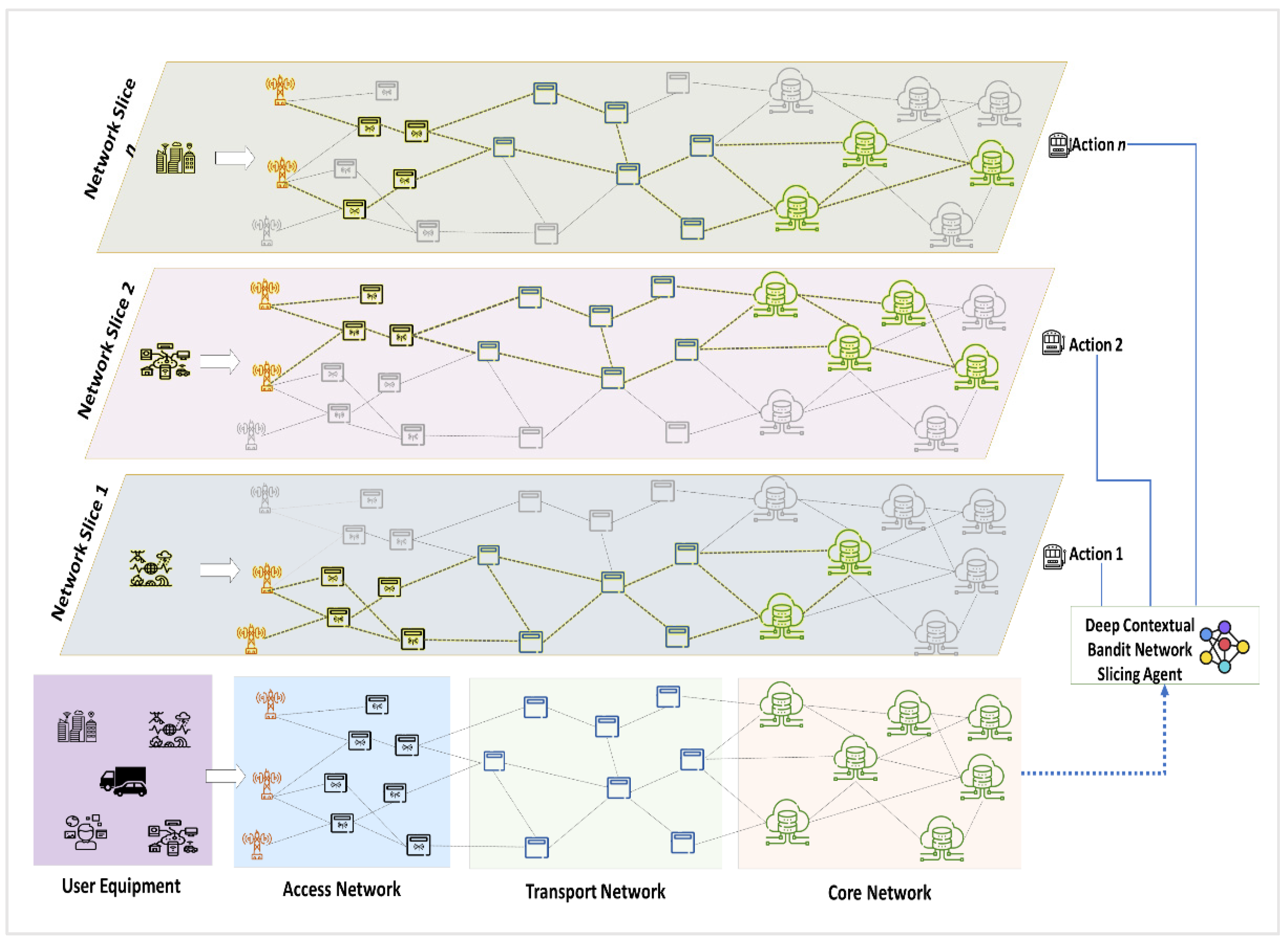
Figure 1 illustrates the system architecture of the proposed DCB-NS scheme. The proposed architecture divides the 5G network model into access, transport, and core networks. The main access point for users is through the access network. Next, the transport nodes forward service requests to the core network. Then, all service requests in the form of NSRs are processed in the core network, where the DCB-NS agent provisions appropriate network slices.
The proposed NS architecture consists of a set of physical nodes such as base stations, network switches, edge servers, and core computing servers , physical links } which are either wired or wireless, and user equipments . The network provides each node with a CPU computing capacity C. On the other hand, the network links are provided with link capacity B, measured in the allotted bandwidth per link. Lastly, the user equipments represent the devices (IoT devices, smartphones, and autonomous vehicles) that access and send NSRs to the 5G network.
3.2. Network Slice Request Model
The NSR of user at time is represented as with eMBB, mMTC, and uRLLC slice requests denoted by , and , respectively. For each slice request , the user requests a specific amount of computing capacity (number of CPU cores) and link capacity (MHz) from the network based on the service or application they use. Additionally, each NSR includes the number of nodes , a minimum transmission delay (milliseconds), the number of physical links (either wired or wireless) , and the request lifetime (seconds) as request parameters. For example, we denote the uRLLC NSR for a user as . Furthermore, based on this model, the network will be able to identify the resources required by a user for each NSR and handle such requests by allocating the necessary resources through a network slice.
3.3. Node Selection and Slice Mapping Model
The node selection method is based on network theory [
27,
28] and uses node degree and centrality values to select candidate nodes for
. These parameters are chosen to select the nodes with the optimal position in the network. Accordingly, the degree of a node refers to the number of connections adjacent to other nodes in the network. Each node
has two degrees: an out-degree, which refers to the number of outgoing edges,
and an in-degree of the number of incoming edges onto
,
where
is equal to 1 if node
is directly connected to node
, and 0 if otherwise. The total degree of a node is then calculated as,
A centrality analysis is then performed for each node to determine its degree of importance to the information flow in the network. In this study, the betweenness centrality of the node is the chosen measure. We are interested in selecting candidate nodes based on how frequently they are used for network information flow. As such, the betweenness centrality of node
i is estimated as,
where
is the number of all paths passing through node
, and
is the sum of all the shortest paths from nodes
to
.
The node’s viability
is then calculated using the values for
and
as in Equation (5),
where the node resource values
for computing capacity, and
for the total link capacity for all links of
are considered. All
ξ values are stored and arranged (in descending order) in the node viability array (NVA) to be used later for candidate node selection. Moreover, sorting from the highest value to the lowest means that nodes with higher
values are given priority for candidate node selection (Algorithm 1).
| Algorithm 1. NSR Node Selection Method. |
| 1: | initialize , , , , , and x values |
| 2: | for each node i with : |
| 3: | calculate node degree (Equation (3)) |
| 4: | calculate node betweenness centrality (Equation (4)) |
| 5: | calculate node viability value (Equation (5)) |
| 6: | save of node to NVA |
| 7: | sort NVA values in descending order |
| 8: | for each : |
| 9: | input x value as the number of nodes to select from NVA |
| 10: | while : |
| 11: | retrieve from NVA |
| 12: | return and perform node mapping (Algorithm 2) |
For the mapping of paths that interconnect network nodes, conventional approaches use the shortest path methods [
20,
23,
28] such as breadth-first search (BFS) and
k-shortest path algorithms. This study implements the maximum flow approach utilizing the Edmonds–Karp method [
29]. The network’s maximum flow indicates the amount of data that can flow through the network’s connections at a given time. This approach calculates the network’s flow by taking the sum of available bandwidth for all edges in the network. Additionally, this process aims to find all feasible paths or augmenting paths
from source node
to target node
for every
while considering the link capacity of every edge in the network. Such an approach reduces the chances of congestion when there is an influx of requests in the network. The nodes ranked in the NVA are used as target nodes for the link mapping process using the Edmonds–Karp method. Furthermore, choosing the best path for the selected nodes requires satisfying the following inequalities,
where
is the total residual flow (in terms of link capacity) for path
from the source node to the target node for
,
is the length of path
,
is the average path length for all node connections, and
is the total roundtrip time for data transmission from the source to target node expressed as,
where
and
refer to the transmission times from the source node to the target node, and from the target node to the source node, respectively. These transmission times denote the amount of time required for the NSR to travel from the source node to the target node (vice-versa) and is affected by transmission delays.
Algorithm 2 presents the details of the link mapping method. This approach aims to find the best path to the target node
for
. Equation (6) ensures that the length of this path does not exceed the average length of all paths in the network. Equation (7) guarantees that the residual flow meets the required link capacity for
. In addition, Equation (8) ensures that the total time needed to transmit
from
to
(vice-versa) does not exceed the specified lifetime of the NSR. Furthermore, all identified augmenting paths are used as links for candidate network slices by the DCB-NS agent for NSR slice provisioning.
| Algorithm 2. NSR Link Mapping Method. |
| 1: | initialize flow value |
| 2: | for each value from NVA: |
| 3: | select source node and initialize node of as target node |
| 4: | let be a path with the minimum number of edges |
| 5: | perform Breadth-First Search for to |
| 6: | for each in : |
| 7: | calculate for residual flow |
| 8: | , for forward
edges |
| 9: | , if otherwise |
| 10: | if Equations (6)–(8) = true: |
| 11: | store to augmenting path array |
| 12: | select with highest from as NSR path |
| 13: | return |
3.4. Deep Contextual Bandit Network Slicing Scheme
Reinforcement learning (RL) methods facilitate agent learning through evaluative feedback. An action performed by an agent is evaluated based on its quality, for which it receives a corresponding reward. In addition, RL agents attempt to solve a problem by balancing exploitation and exploration of actions. This process, in turn, allows the agent to learn a strategy to obtain an optimal reward for each action. Additionally, the way RL agents learn is in direct contrast to other AI methods that guide the agent to take corrective actions based on existing training data.
This work implements a variant of the multi-armed (or
k-armed) bandit approach known as Contextual Bandits [
30] for the proposed NS scheme. This approach is a type of associative search method in which the current state of the environment affects an agent’s reward for a given action. A famous example of this scenario is the case of slot machines in a casino, where a player tries to get the best payoff while playing slot machines. In this scenario, the rewards for pulling the arm of a slot machine (or bandit) are randomly distributed and are unknown to the player, so the player must choose the best action strategy to get the best payoff. Therefore, we model the proposed scheme based on a Contextual Bandit scenario. Moreover, a deep reinforcement learning is utilized to compute the reward and formulate the action strategy efficiently through a trial-and-error approach. The deep neural network receives the NSR parameters as through its input layer and then outputs it through the output layer. The rewards are calculated based on the network’s current state and checked for errors or losses using the mean squared error method. Such an approach leads to an optimal resource allocation strategy in the form of a network slice for each NSR. A graphical representation of the Deep RL model is shown in
Figure 2.
The proposed scheme considers an input
, and a set of actions
, and each action
has an associated reward
. In this case,
and the mapped nodes
represent the input and the agent’s actions, respectively. For every action taken, the agent expects to achieve a value or utility
that measures the quality of such action. This value or utility calculation is expressed as,
thus, the expected value
for action
is equivalent to the reward for that action at time
. In addition, the actions in the agent’s action space are randomly distributed using a Softmax function, which is denoted as,
where the probability of choosing an action is calculated by dividing the input vector’s exponential function
over the sum of all the exponential functions for an output vector
for a
number of classes. Moreover, this probability distribution method enables the NSA to randomly select an action out of a given set of possible actions without any bias.
Since the Contextual Bandit approach considers the environment state to determine the reward for an action taken, it is also necessary to define state as a set of states where each state comprises various reward influencing factors (RIF). The various factors are defined as follows:
- 1.
The total path length
is the sum of all paths from
to
. This value provides the agent with the candidate slice topology information.
- 2.
The computing capacity utilization denoted as
provides information regarding the computing capacity
allocated for
at time
. This value also helps determine the remaining computing capacity for the network’s physical infrastructure at the specified time step.
where
refers to the total remaining computing capacity for all physical infrastructure nodes.
- 3.
The bandwidth utilization
reflects the network’s total bandwidth utilized at time
. This bandwidth utilization is also affected by other NSRs served at the specified time step.
where
is the allocated link capacity for
and
is the total remaining link capacity for all nodes from the physical infrastructure.
- 4.
Node utilization
represents the percentage of network nodes serving all existing NSRs at time
. It also verifies whether the network can allocate the nodes needed by the NSR.
where
is the number of allocated nodes for
at time
and
is the total remaining number of physical infrastructure nodes.
Using RIFs as weights whose values are determined by the network state, the reward
for action
is calculated as
where
is a weight factor defined by the network’s current state. We have defined the following network states
to find for reward
as follows:
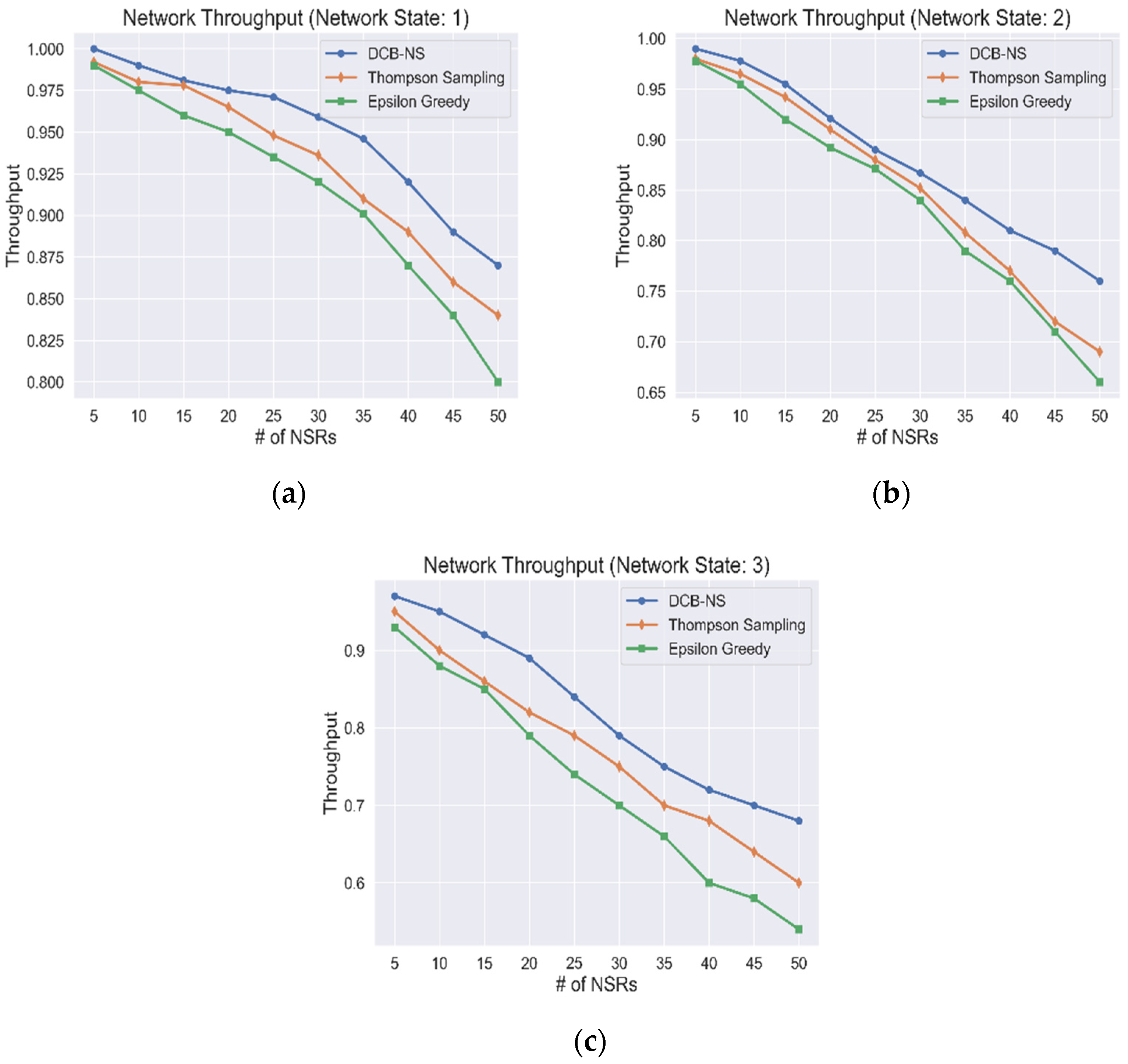
- 1.
Network State 1 () represents a normal network state, meaning that the total available computing capacity , link capacity , the number of usable nodes , and total path length are at 81–100%.
- 2.
Network State 2 () indicates that , , , and are at 50–80% capacity or availability. Such a state requires that succeeding NSRs should not exceed the remaining capacity of available network resources.
- 3.
Network State 3 () signals that all network resources are below 50% capacity or availability. This state indicates either that the network is currently serving many NSRs or the NSRs currently served are utilizing a large amount of resource capacity.
Based on these network states, a combination of values for each
of a RIF is assigned in
Table 2.
The weight assignments in
Table 2 show that
requires a careful allocation of resources for an NSR to avoid network failure. State
, on the other hand, prioritizes resource allocation for computing capacity and bandwidth to incoming NSRs. Finally,
has a lower priority on resource allocation since the network has high resource availability.
Next, the accumulated reward for a specific action
at time
is denoted as
and then calculated after exploring all possible actions from the action space as,
where
is the number of instances performed by the agent for action
, and
is the reward earned for each action.
The Upper Confidence Bound (UCB) strategy is utilized to facilitate the exploration and exploitation of actions. Through this, the agent decides whether to continue choosing an action that gives a particular reward value (exploitation) or to check for other possible actions that could yield higher rewards (exploration). The UCB for action
is expressed as follows,
where
is the number of instances when action
is chosen before time
, and
is a predefined confidence value controlling the degree of exploration. The UCB strategy implies that by checking each action’s
and the number of instances it was executed, it can exploit the action with the highest
. However, other possible actions are explored and re-evaluated.
The calculated rewards are then evaluated for every action the agent performs to assess its quality. At the end of the training period, the cumulative mean rewards
for each action are taken as,
where
Y denotes the number of instances when the agent chose action
. These values are then ranked in descending order, and the action with the highest
is implemented as a network slice
. Finally, the proposed DCB-NS scheme details are presented in Algorithm 3.
| Algorithm 3. Proposed Deep Contextual Bandit Network Slicing Scheme. |
| 1: | initialize , , , |
| 2: | perform Node Selection (Algorithm 1) |
| 3: | for x in NVA: |
| 4: | perform Node Mapping (Algorithm 2) |
| 5: | add mapped nodes to candidate slices array |
| 6: | check for network state |
| 7: | while : |
| 8: | select action a candidate slice from Slices[] as action |
| 9: | calculate action value (Equation (10)) |
| 10: | calculate reward (Equation (16)) |
| 11: | calculate total estimated value (Equation (17)) |
| 12: | calculate Upper Confidence Bound (Equation (18)) |
| 13: | if = 1: |
| 14: | set of as the max UCB |
| 15: | select new action , repeat steps 8–12 |
| 16: | else: Compare values for all actions performed |
| 17: | if of current action is highest: |
| 18 | set of that action as max UCB (exploit) |
| 19: | else: select new action and repeat from step 8 (explore) |
| 20: | select action with the highest from all actions performed in |
| 21: | implement selected action as network slice for |
| 22: | return |


