1. Introduction
The goal of this paper is to evaluate the radiative fluxes for the greenhouse effect in the atmosphere. This evaluation is based on a developed algorithm formulated in [
1]. The used model includes the following features.
1. The “line-by-line” model [
2,
3] is the basis of these evaluations, and integral radiative fluxes follow from these partial fluxes.
2. The model includes three basic greenhouse components, namely, molecules, molecules and liquid water microdroplets, as the basic condensed phase in the atmosphere. In addition, trace components, such as molecules and molecules, may be included in this scheme.
3. The model of standard atmosphere [
4] is the basis of evaluations. In particular, the global temperature (the average temperature of the Earth’s surface) is taken as
K, and its decrease with altitude
h is
K/km. This model provides the altitude distribution for the number densities of atmospheric molecules. The model of standard atmosphere implies that atmospheric parameters depend only on the altitude.
4. Along with the local thermodynamic equilibrium for atmospheric components, this equilibrium takes place between the radiation field and atmospheric air.
5. Parameters of radiative transitions of greenhouse molecules are taken from the HITRAN data bank [
5,
6,
7]; therefore, we use the formalism for the rates of molecular radiative processes of this data bank [
8].
6. The energetic balance of the Earth and its atmosphere is taken into account. According to this balance, radiative fluxes toward the Earth and outside are determined by different atmospheric regions and are separated, i.e., the radiative fluxes to the Earth that are connected with its temperatures do not depend on processes in high layers of the troposphere.
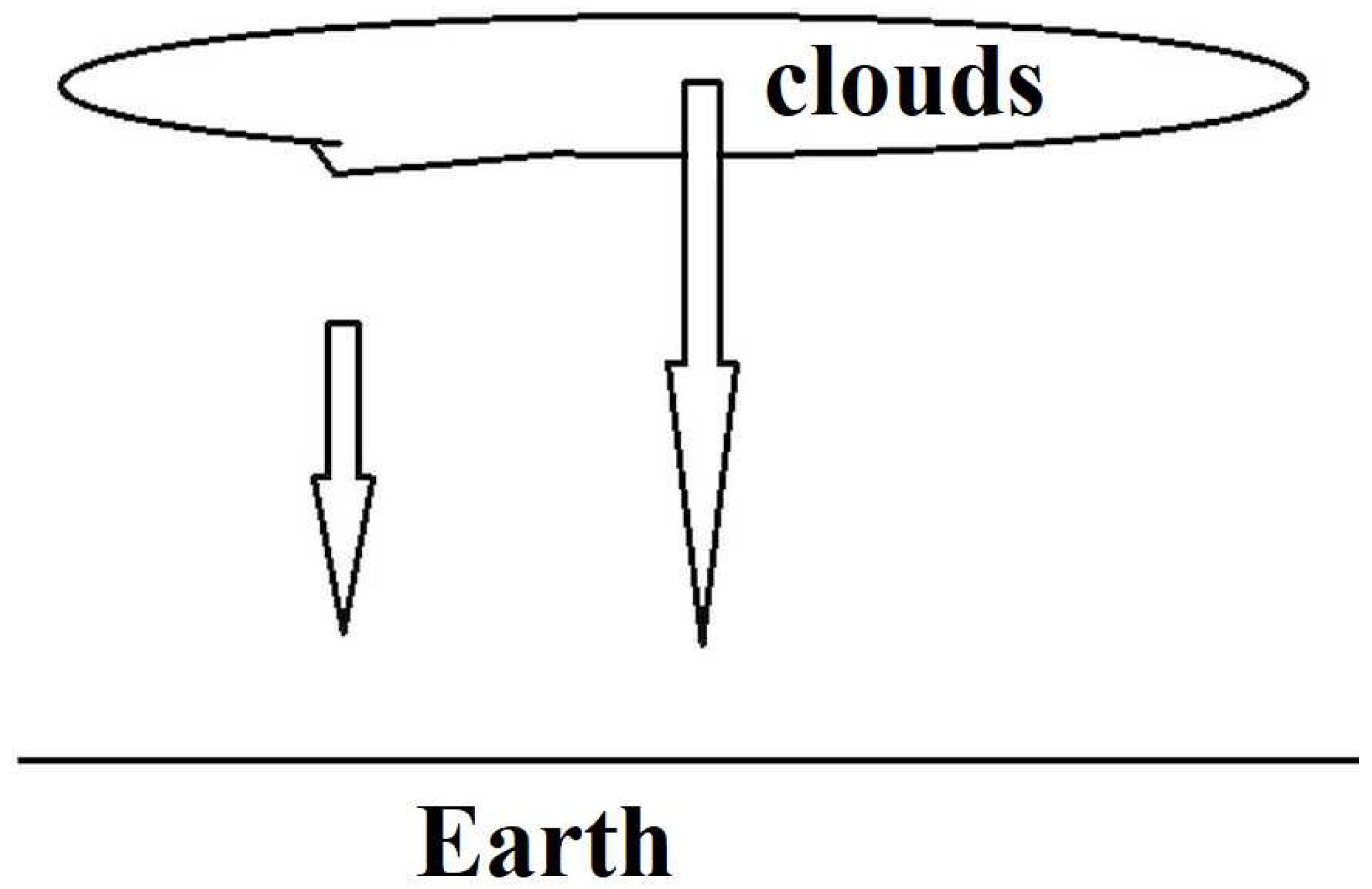
7. Basic greenhouse components are separated so that clouds are located starting from a certain altitude, and they are characterized by a sharp boundary. Radiation from greenhouse molecules is created in the gap between the Earth’s surface and clouds.
Differences between these evaluations and those of [
1] are twofold. First, the computer code presented in our paper does not separate frequencies in different ranges; this code relates to the total range of frequencies. Second, evaluations [
1] are restricted by frequencies below 1200 cm
. Since the absorption in an additional frequency range is determined by water molecules, new evaluations may change the emission, due to water molecules. Of course, we account for this in our analysis for a contemporary understanding of atmospheric physics and processes in the atmosphere [
2,
3,
9,
10,
11,
12,
13,
14,
15,
16,
17,
18,
19,
20,
21,
22].
2. Model of Atmospheric Emission to the Earth
Thus, we evaluate the radiative fluxes on the basis of the algorithm, which is formulated in the introduction section. The character of radiative processes is given in
Figure 1. Correspondingly, according to the model under consideration, we have for the radiative flux
at a given frequency
the following:
where
is the radiative flux of a blackbody with a temperature
T at this frequency that is given by the Planck formula as follows [
23,
24]:
and the opaque factor
of a uniform gaseous layer is given by the following [
25,
26]:
Formula (
3) takes into account the thermodynamic equilibrium of air molecules of the atmosphere with its optically active molecules, water microdroplets of clouds, and the radiation field.
We thus consider the radiating atmosphere as a shell of the Earth, whose thickness is small compared with the radius of the Earth. Hence, the radiating atmosphere is a weakly nonuniform gaseous layer [
27]. One can reduce a radiating weakly nonuniform layer that contains optically active molecules to an effective uniform layer by introducing the effective temperature of radiation or the radiative temperature
[
28,
29]. In addition, due to thermodynamic equilibrium in the atmosphere, the emission of clouds is characterized by the cloud + temperature
or the temperature of the cloud boundary because of its sharp structure.
Formula (
1) contains parameters that are expressed through the optical thickness
of the radiated atmospheric layer, which in turn is connected with the optical parameters of optically active molecules, which are located in atmospheric air. There are three greenhouse parameters of the radiated atmospheric layer, namely,
molecules,
molecules, and clouds consisting mostly of water microdroplets. Correspondingly, the optical thickness of the atmospheric gap located between the Earth and clouds is given by the following [
1]:
where the number densities of water molecules and carbon dioxide molecules are determined by the following formulas:
We use here the data of the model of standard atmosphere [
4] and measured data on the basis of the NASA programs, which are analyzed in [
30]. In addition, the equation for the effective altitude
at a given frequency
has the following form [
1]:
Within the framework of the model of standard atmosphere, the radiative temperature
for a given frequency follows from the given relation:
where the global temperature equals
K for the contemporary standard atmosphere, and its gradient is
K/km.
Formula (
4) includes the absorption cross section
for molecules of a given sort, which is a sum of the cross sections for individual spectral lines due to this component, according to the following formula:
As is seen, for each radiative transition, this formula contains three parameters, namely, the transition intensity
, the frequency
at the line center, and the width of this spectral line
. We take these parameters from the HITRAN data bank [
5,
6,
7], and these parameters allow one to determine the absorption cross section at a given frequency. In addition, for air pressures under consideration which are of the order of atmospheric one, the following criterion is fulfilled:
where
is a typical difference of frequencies for centers of neighboring spectral lines.
Note that, according to the Wien law [
31], the maximum flux of photons for a blackbody corresponds to the wavelength
as follows:
From this, it follows that a typical wavelength of atmospheric radiation is m. Therefore, below, we are restricted by frequencies .
In this evaluation, we are guided by strong spectral lines such that at the centers of these lines, the optical thickness satisfies the relation
. In accordance with typical parameters of spectral lines due to water and carbon dioxide molecules, one can select from the HITRAN data bank radiative transitions for these molecules whose intensities satisfy the following relation:
The problem in the evaluation of the radiative flux of the atmosphere is determining the parameters of clouds. In contrast to the number densities of optically active molecules, which are given by Formula (
4), analogous information for clouds is absent. Indeed, clouds exist over a given surface point during a restricted time, and their distribution over altitudes has a random character. Within the framework of the model under consideration, we use one parameter of clouds, namely, the altitude
, which determines the radiation of clouds, or the radiative temperature of clouds
, which follows from the given equation below:
where the global temperature is
K, and the temperature gradient is
K/km.
One can determine the cloud parameters of this model by using the energetic balance of the Earth and atmosphere. The energetic balance includes the radiative flux
from the atmosphere toward the Earth. The energetic balance and this radiative flux follows from different sources, which are presented in
Table 1. The total radiative flux from the atmosphere to the Earth is given by the following:
This analysis is used below for calculating the partial radiative fluxes from the atmosphere to the Earth.
3. Radiative Fluxes from the Standard Atmosphere
Evaluations of the radiative fluxes from the atmosphere to the Earth are based on the above algorithm [
1]. In the previous analysis, the frequency range was separated over several ranges, and evaluations were fulfilled in each range independently. In this case, within the framework of a general computer code, one can make calculations in the total range of frequencies that determine the radiative flux. Let us choose the effective range of flux evaluations. If the Earth’s surface with the temperature of the standard atmosphere
K emits as a blackbody, the radiative flux at frequencies above 1300 cm
is
of the total radiative flux, the radiative flux at frequencies above 2000 cm
is
of the total radiative flux, and the radiative flux at frequencies above 2600 cm
is
of the total radiative flux. In previous evaluations [
1], calculations were made for frequencies below 1260 cm
, accounting for the radiation of molecules
,
and
at larger frequencies. We are now restricted by the frequency range below 2600 cm
.
By analogy with evaluations [
1], in subsequent calculations, we use information about radiative transitions from the HITRAN data bank.
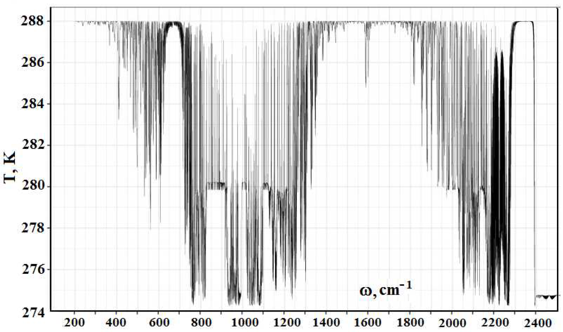
Figure 2 contains the frequency dependence for the optical thickness of the atmospheric layer between the Earth’s surface and clouds, which is determined by optically active atmospheric molecules in the infrared spectrum range. As it follows from this Figure, optical parameters of the atmosphere as a frequency function have a line character. One can determine from this the radiative temperature of molecules located in the atmospheric gap between the Earth and clouds, and its frequency dependence is presented in
Figure 3.
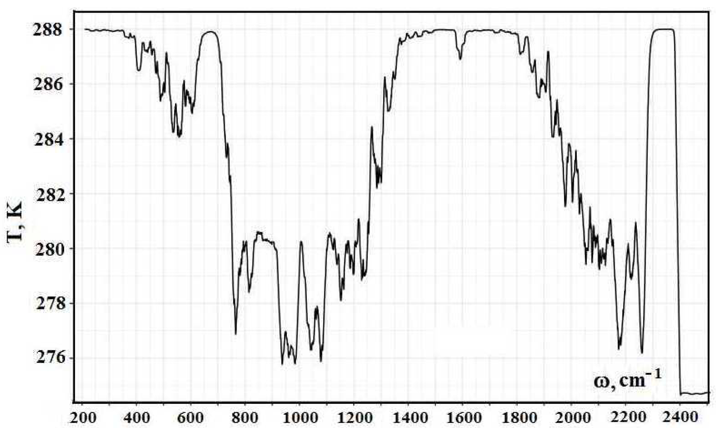
Figure 4 contains values of radiative temperatures, given in
Figure 3, which are averaged over ranges of 20 cm
width. This averaging is made over the frequency range of the width of 10 cm
below and above the frequency under consideration.
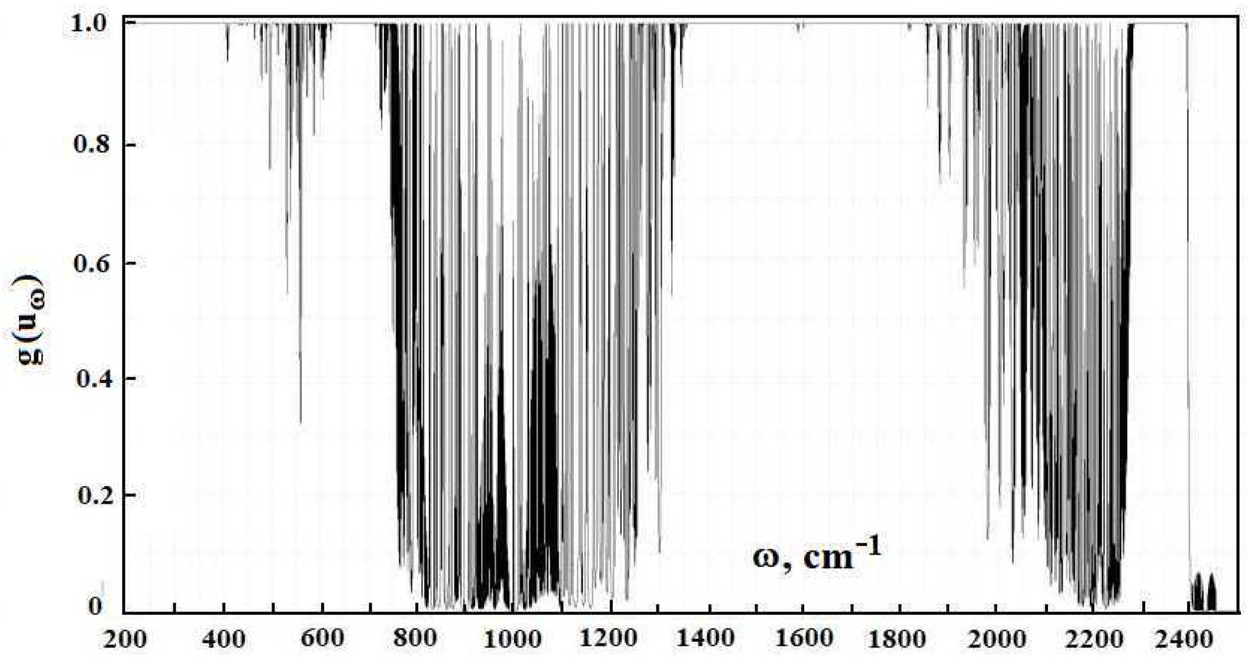
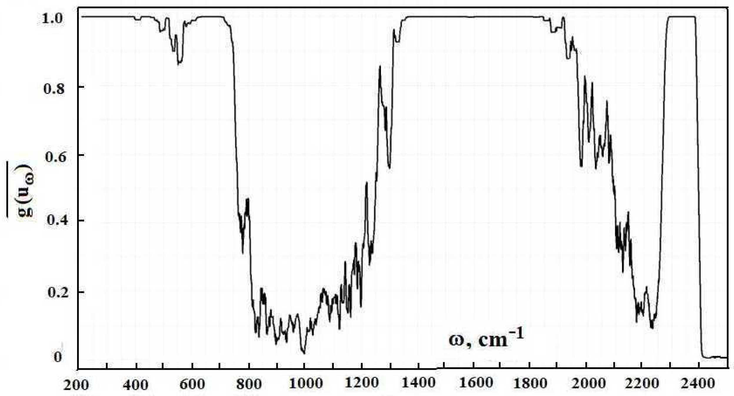
The opaque factor
is determined by Formula (
3), and its frequency dependence is given in
Figure 5. The averaged value of the opaque factor is given in
Figure 6. The averaging is made over the frequency range of 20 cm
by analogy with that for the radiative temperature.
The opaque factor characterizes the part of the radiative flux that is emitted by the Earth’s surface and attains the clouds.
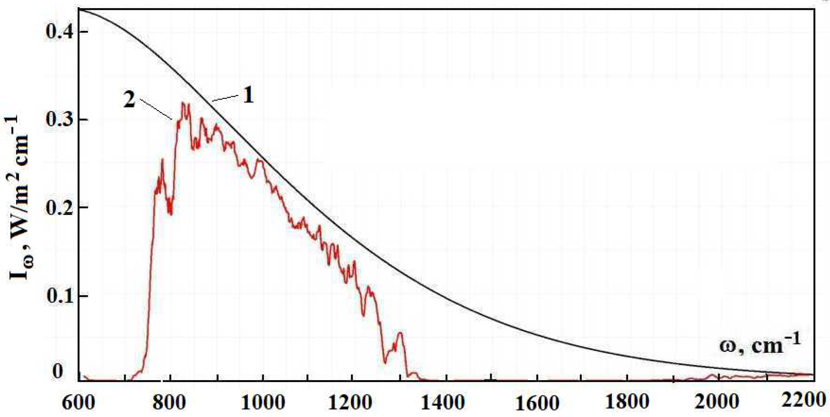
Figure 7 contains the radiative flux
that is emitted by the Earth as well as the radiative flux
at a given frequency, which reaches the clouds for the model of standard atmosphere. We have also the average radiative flux, which is emitted by the Earth and reaches the cloud boundary as follows:
Taking
K on the basis of the model of standard atmosphere, we obtain the following:
in accordance with the energetic balance of the Earth, and
W/m
. As is seen, a part of the thermal radiative flux that passes through the atmospheric layer below clouds and reaches the clouds is approximately
of the emitted radiative flux.
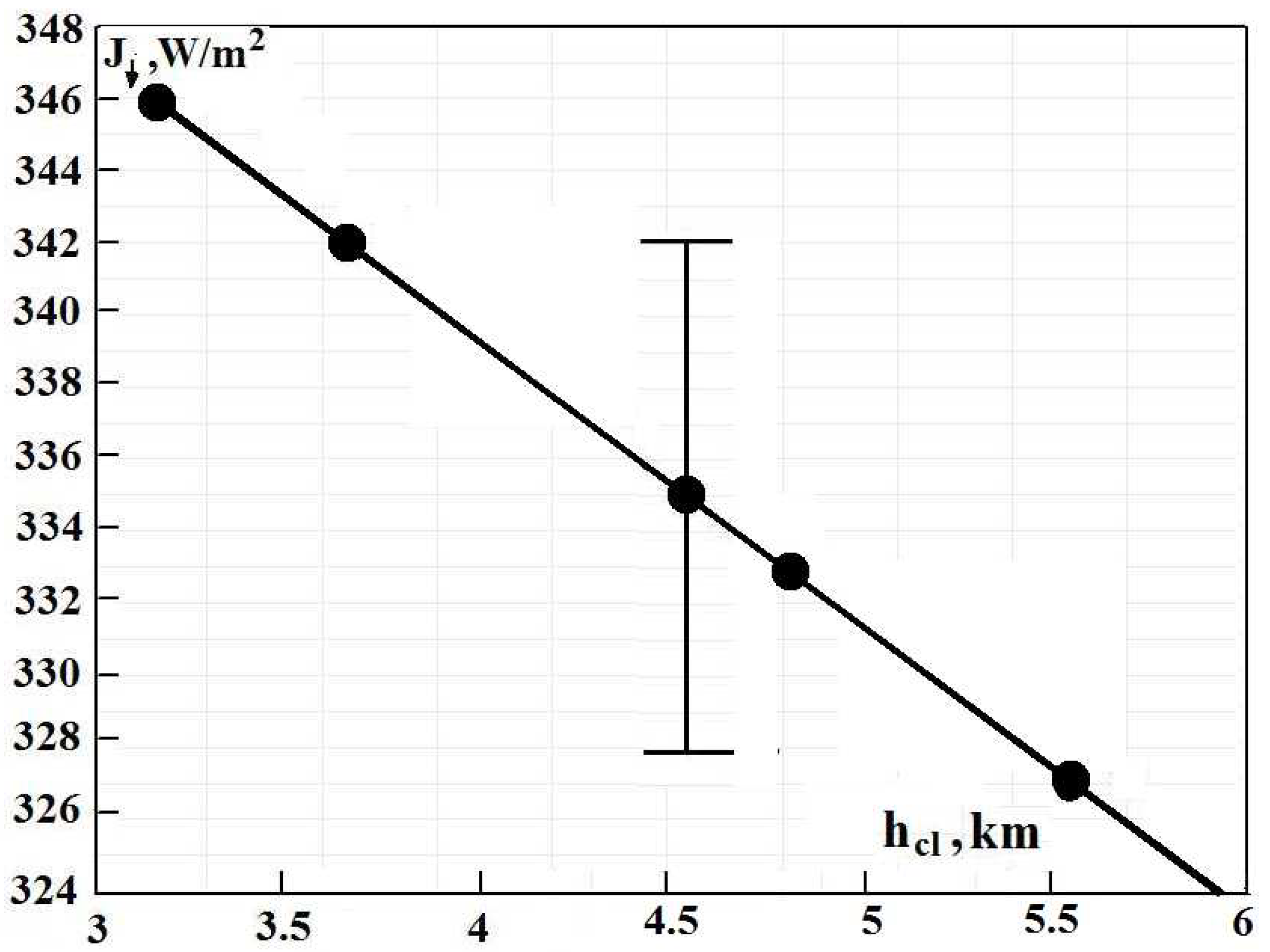
From Formulas (
1) and (
13), one can determine the radiative flux from the atmosphere to the Earth’s surface due to atmospheric molecules and clouds; this flux depends on the cloud temperature
or the boundary altitude
for clouds. This dependence is represented in
Figure 8. In addition, these parameters are given in
Table 1 for different versions of the energetic balance of the Earth and its atmosphere.
In previous evaluations [
1], only data of the first source of
Table 1 were used, whereas now we are based on a variety of these values. Because parameters of the Earth’s energetic balance are different for these sources, this difference characterizes also the error in the final results. Note that the connection between the effective altitude
of the cloud boundary and the cloud temperature
is given by Formula (
12).
A cursory glance at the emission parameters of the atmosphere according to
Figure 2,
Figure 3 and
Figure 5 exhibits that the spectrum of atmospheric radiation consists of separate spectral lines, in contrast to climatological models with a smooth empiric frequency functions, which approximate the atmospheric spectrum. In addition, climatological models do not take into account the thermodynamics of the atmosphere and radiation field. Therefore, computer codes of climatology are not reliable in the evaluation of the radiative parameters of the atmosphere.
One can divide the radiative flux
from the atmosphere to the Earth in parts that are created by various components of the radiated atmosphere. For example, the partial radiative flux
, which is determined by
molecules, is given by the following formula:
where
is the total radiative flux,
is the absorption coefficient due to
molecules, and
is the total absorption coefficient at a given frequency. These absorption coefficients are taken at the radiative temperature
. Integrating the partial radiative flux as a frequency function over frequencies, one can determine the total radiative flux from the atmosphere to the Earth due to this component.
Table 2 contains values of the total radiative flux from the atmosphere due to each greenhouse component.
One can compare the results for radiative fluxes of these evaluations given in
Table 2 and previous ones [
1]. The basic difference is that the basic part of the emission, according to [
1], is taken from the frequency range
cm
; in the other frequency range
cm
, which gives the contribution approximately
to the radiative flux, the emission of water molecules is ignored. In these evaluations, the HITRAN bank data are included up to
cm
. As a result, a part of the emission transfers from clouds to water molecules. We also note that average radiative fluxes given in
Table 2, according to evaluations [
1], refer to the total radiative flux
W/m
from the atmosphere toward the Earth, whereas now, we are guided by this flux
W/m
; the results of
Table 2 correspond to the total flux.
In addition,
Figure 9 contains radiative fluxes due to individual greenhouse components. The frequency range is separated into two parts with the boundary of 800 cm
. One can evaluate separately the emission of trace greenhouse components, which are
and
molecules. The number density of these molecules as an altitude function is analogous to formula (
5) for
molecules and is given by the following formulas:
The number densities of these molecules at the Earth’s surface are taken from [
47,
48]. The absorption band for the
molecule is (1240–1360) cm
, the absorption bands for
molecule are placed in the frequency ranges (1250–1310) cm
and (2180–2260) cm
.
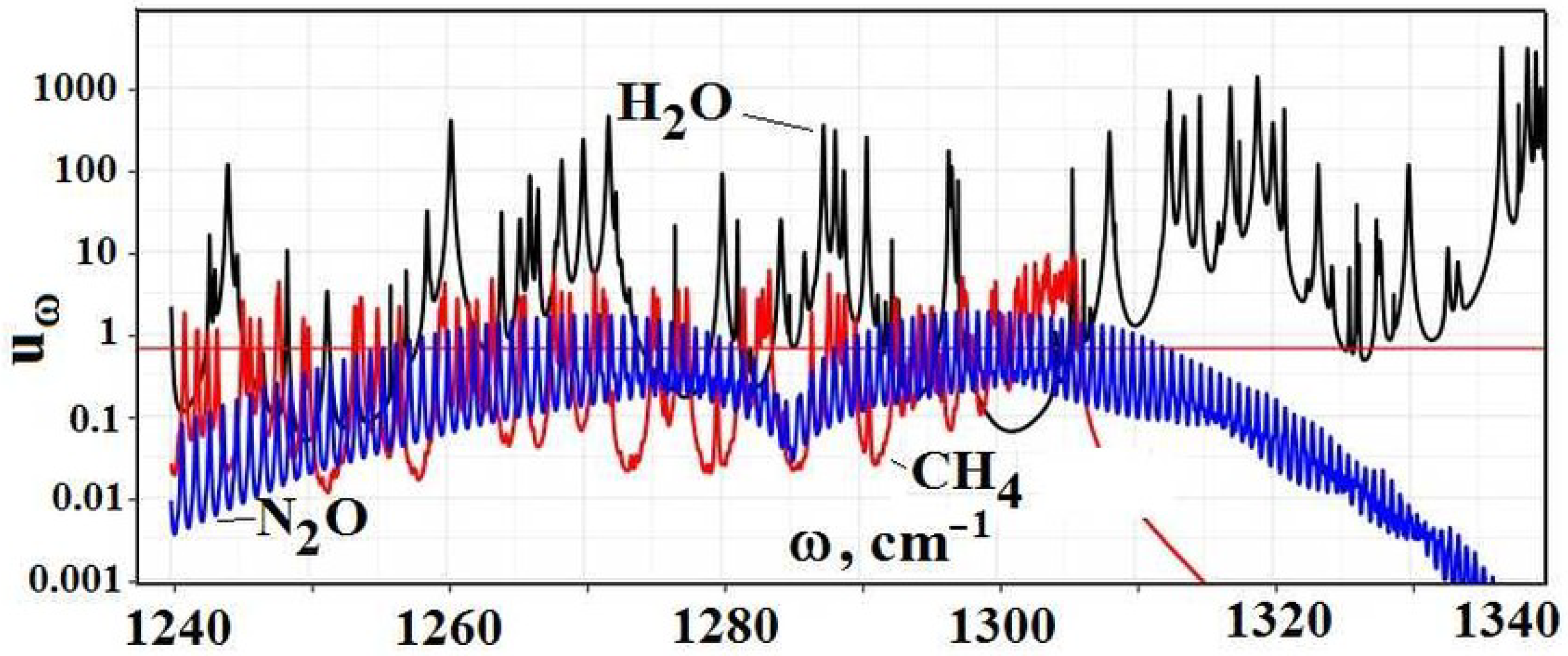
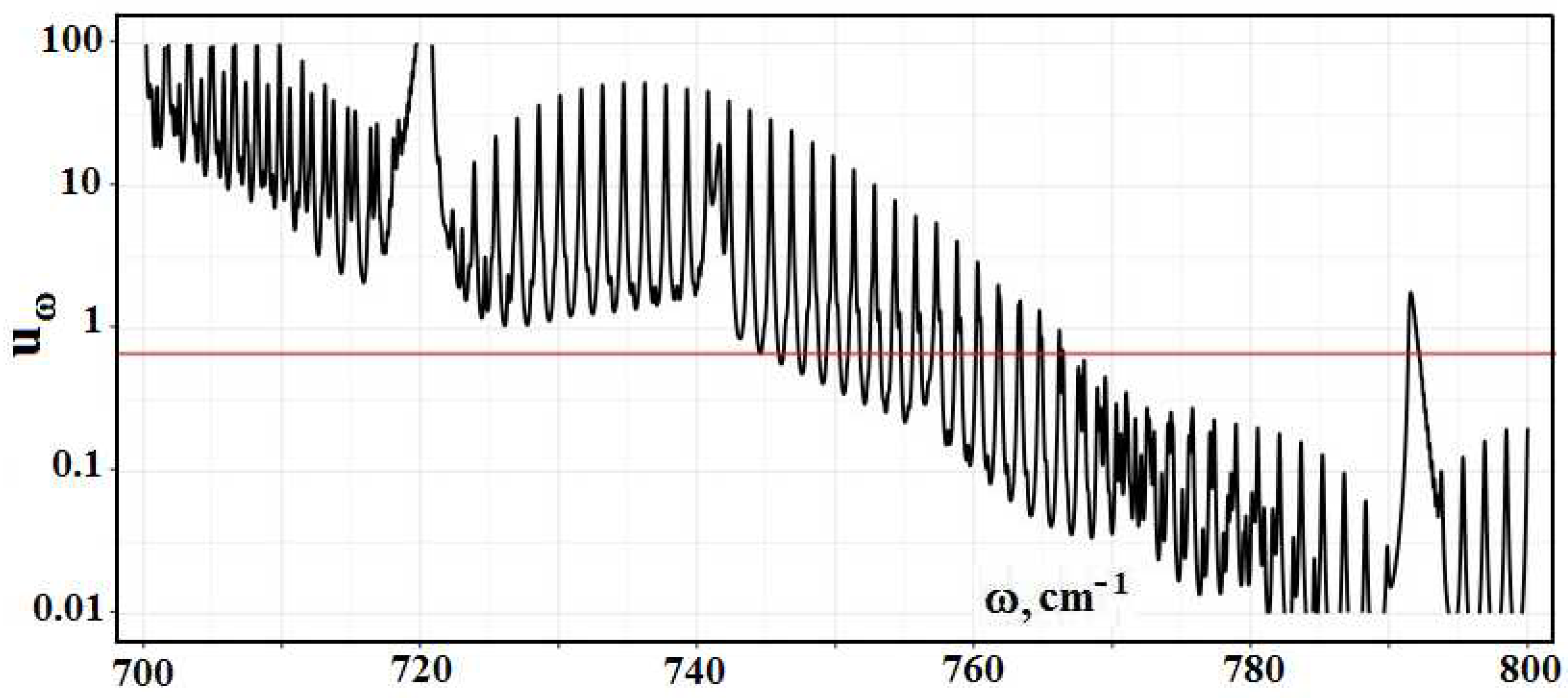
Figure 10 contains the partial optical thickness as a frequency function in the above absorption bands, due to individual greenhouse components, which include the above trace components and water molecules.
As it is seen, the optical thickness due to trace gases is not large and is screened by absorption of water molecules. Because we ignored in [
1] the absorption of water molecules at the wing
cm
of atmospheric thermal emission, evaluations [
1] contain heightened values of radiative fluxes due to trace gases, as it follows from the data of
Figure 9 and
Table 2.
It should be noted that we exclude the ozone emission from the tropospheric radiation toward the Earth since the concentration of ozone molecules in the troposphere usually does not exceed cm. Therefore, the optical thickness of the troposphere in the gap between the Earth’s surface and clouds is small. The concentration of ozone molecules in the stratosphere is larger, but the stratospheric radiation does not reach the Earth because it is absorbed by clouds. Hence, we ignore the radiation of ozone molecules in the atmosphere.
4. Emission of Atmosphere with a Varied Composition
The code under consideration allows one to analyze variations in the radiative fluxes as a result of the change in the atmosphere composition. We start this analysis from the standard case, where the concentration of
molecules is doubled. This leads to the change in the global temperature that is named “Equilibrium Climate Sensitivity” [
49]. Note that this operation implies that optically active gases have a uniform distribution over the globe that corresponds to the average altitude distribution. This criterion is fulfilled more or less for
molecules, and the uniform distribution is violated for
molecules.
In this consideration, we take into account three basic greenhouse components, namely,
molecules,
molecules, and water microdroplets of clouds.
Table 3 contains the distribution over the spectrum for the change in radiative fluxes due to a given component as a result of doubling the concentration of
molecules. Quantities
,
,
of this table are the changes in the radiative fluxes to the Earth due to
molecules,
molecules, and water microdroplets of clouds, correspondingly, according to the following relations:
where
is the radiative flux due to an indicated component
A at the current concentration of
molecules, and
is the radiative flux of this component at the doubling concentration of
molecules. The change in the total radiative flux
is introduced as follows:
It is evident that the change in radiative fluxes of components as well as the total change in the radiative flux from the atmosphere to the Earth takes place only in spectrum ranges where
molecules absorb. In addition, the basic change in the radiative flux as a result of the concentration change for some optically active components takes place in the frequency range where the optical thickness is of the order of one. The red line
in
Figure 2,
Figure 10, and
Figure 11 separates the optical thicknesses, with large ones above this line and low ones below it. Comparing the data of
Table 3 and
Figure 11, one can conclude that the main contribution to the change in the radiative flux follows from a frequency range where
. Next, changes in radiative fluxes resulted from the variation in the concentration of
molecules are nearby, according to these calculations and evaluations [
1], because the absorption of
molecules is absent in the added frequency range 1200 cm
cm
. On the contrary, in the case of the change in the concentration of water molecules, the change in the total radiative flux differs by several times under identical conditions.
One can see from the data of
Table 3 that the change in the radiative flux
due to
molecules as a result of doubling the concentration of
molecules is five times larger than the change in the total radiative flux
. In climatological models, the Kirchhoff law [
50], according to which radiators are simultaneously absorbers, is ignored. Therefore, the change in the radiative flux
due to
molecules is taken in climatological models instead of the change in the total radiative flux
, and the error in the change of the global temperature under these conditions is exceeded by five times. This results from neglecting the absorption of emitted radiative fluxes by water molecules and water microdroplets of clouds by added
molecules [
51,
52]). This large difference follows also from a general conclusion for a plane gaseous layer with a low temperature gradient [
51,
52]). Indeed, if we have a layer of a constant temperature and of a high optical thickness, where the emission is created by several components, this layer emits as a blackbody with the gaseous temperature. Therefore, a change in the concentration of some optically active component would not lead to the change in the outgoing radiative flux.
A comparison of the results of these evaluations with those of [
1] allows one to estimate the accuracy of the change in radiative fluxes, which is estimated as ∼
. The same accuracy corresponds to the derivative of the radiative flux over the concentration of a given component. From these calculations, in the case that the concentration of
molecules varies, while other atmospheric parameters are unvaried, we have the following:
where
is the radiative flux from the atmosphere to the Earth, and
is the concentration of
molecules.
Along with variations in the concentration of
molecules, other changes take place in the real atmosphere, which influence the global temperature. Let us analyze this change in the real atmosphere on the basis of measurements within the framework of NASA programs. We use below the results of measurements for the concentration
of carbon dioxide molecules [
53,
54]. Because the time of residence of a
molecule is large, we take the evolution of the atmospheric concentration of
molecules according to measurements in the Mauna Loa observatory as the global evolution of this quantity. Next, the evolution of the global temperature during the last 150 years is analyzed carefully by the Goddard Institute for Space Studies (GISS) (for example, [
55]) within the framework of the NASA program. These results are collected in [
1] and are as follows:
One can connect the change in the radiative flux from the atmosphere to the Earth
and the change in the global temperature
through climate sensitivity
S, according to relation [
18,
56]:
We use the average value of these quantities, which follows from an average of various data and is
[
1]. One can estimate the accuracy of this value as ≈
. From this, for the derivation of the radiative flux
over the concentration of
molecules (
) in the real atmosphere, we have the following:
We note that in contrast to formula (
19) where all atmospheric parameters, except for the concentration of
molecules, are unvaried, formula (
22) takes into account other processes that lead to the change in the global temperature. As is seen, the contribution of carbon dioxide in the change in the global temperature for the evolution of the real temperature is approximately
.
By analogy with the
case, one can analyze the influence of the change in atmospheric water molecules on the change in the radiative flux from the atmosphere to the Earth. Some results that are analogous to those of
Table 3 are given in
Table 4. From the data of this table, we have the following:
where
is the concentration of atmospheric water molecules.
Let us assume that along with an increase in the concentration of
molecules, the evolution of the global temperature of the real atmosphere is determined by the increase in the concentration of
molecules. Then, water molecules account for the contribution of
of the change in the global temperature. On the basis of Formula (
20), we have the following:
where
is the part of the global temperature change which follows from an increase in the concentration of
molecules. Taking as early
, one can find the derivation part of the radiative flux from the atmosphere to the Earth due to
molecules as follows:
From this, it follows the rate of variation for the concentration of the water molecules
, which can provide this change:
According to this result, the observed rate of an increase in the global temperature may be determined by an increase in the following average number density of water molecules:
The annual change in the number density is small, compared to the contemporary number density of water molecules, which is equal to . Therefore, a real determination of this derivation under contemporary conditions is problematic and requires additional efforts similar to those for the evolution of the global temperature.
It should be noted that the moisture
is the measured water parameter in the atmosphere that is given by the following:
where
is the number density of water molecules at the saturated vapor pressure for a given temperature,
is a current concentration of water molecules in atmospheric air, and
is its concentration for the saturated vapor pressure at the air temperature. The contemporary value of the atmosphere moisture is
[
57].
Let us determine the rate of the moisture variation due to the temperature change. Because the amount of atmospheric water is small compared to that at the Earth’s surface, we have, from an equilibrium between the atmospheric and surface water, the following:
where
eV [
58] is the binding energy for a water molecule with its bulk liquid. From this, for the rate of an increase in the atmosphere capacity with respect to water molecules due to a temperature increase, we have the following:
The process of growth of the atmospheric moisture will be stopped through a time
, according to the following equation:
From this, it follows that , i.e., this time is sufficiently large to check this mechanism of the Earth’s heating.
5. Conclusions
The goal of this paper is to apply the improved code for the evaluation of the radiative fluxes from the atmosphere to the Earth on the basis of the model of [
1]. In these evaluations, we use the range of frequencies up to
in contrast to the previous calculations [
1], where this range was restricted by
. Besides this difference, we use now various versions of the energetic balance of the Earth and its atmosphere (see
Table 1), and the difference in radiative parameters due to various versions of the Earth’s energetic balance may be considered an error of the results. Nevertheless, the cloud boundary altitude
, as one of basic parameters of the model under consideration, according to [
1], is
, whereas from
Table 1, the average altitude of the cloud boundary is
km, i.e., these values coincide within the accuracy of these evaluations.
Because carbon dioxide molecules do not absorb in the additional spectrum range between 1200 cm
and 2600 cm
, the radiative parameters due to
molecules are close in these evaluations and in the previous one. In particular, the variation in radiative fluxes as a result of the change in the carbon dioxide amount in the atmosphere for these calculations are close. In this evaluation as well as previous evaluations, we have a contradiction with the results of climatological models in the analysis of the Earth’s greenhouse effect, according to which the increase in the global temperature differs by five times. We show [
51,
52], so the large difference results from ignoring, in climatological models, the Kirchhoff law [
50], according to which radiators are simultaneously the absorbers. In this case, we take the change in the radiative flux created by
molecules as the change of the total radiative flux.
Note the restrictions by the frequency range up to 1200 cm
in the previous calculations [
1]; we thus assume that the atmosphere is transparent for larger frequencies, and the emission at larger frequencies is determined by clouds. However, according to the HITRAN data bank, water molecules absorb effectively in the enlarged frequency range. As a result, the derivative (
22) is larger than that according to [
1]. We proved early (for example, [
1]) that atmospheric
molecules are not the main radiator of the atmosphere. From these evaluations, it follows that water molecules in the atmosphere may be responsible for the observed heating of the Earth.


