Approximating Solutions of Nonlinear Equations Using an Extended Traub Method

Abstract

The Traub iterates generate a sequence that converges to a solution of a nonlinear equation given certain conditions. The order of convergence has been shown provided that the fifth Fréchet-derivative exists. Notice that this derivative does not appear on the Traub method. Therefore, according to the earlier results, there is no guarantee that the Traub method converges if the operator is not five times Fréchet-differentiable or more. However, the Traub method can converge, since these assumptions are only sufficient. The novelty of our new technique is the fact that only the Fréchet-derivative on the method is assumed to exist to prove convergence. Moreover, the new results does not depend on the Traub method. Consequently, the same technique can be applied on other methods. The dynamics of this method are also studied. Examples further explain the theoretical results.

1. Introduction

The article deals with the challenge of approximating a solution $x_{*}$ of the following nonlinear equation:

$$\mathcal{H}\left(x\right)=0,$$

(1)

where operator $\mathcal{H}:\mathsf{\Omega }\subset X⟶Y$ acts between Banach spaces $X,$Y and subset $\mathsf{\Omega }\ne \varnothing .$ Since the analytical form of $x_{*}$ is not easily attainable, iterative methods are considered for solving (1). Throughout the article, $B(x_0,\rho )=\{z\in X:\parallel z-x_0\parallel <\rho \}$ and $B[x_0,\rho ]=\{z\in X:\parallel z-x_0\parallel \le \rho \}$ for some $\rho >0.$ When one studies the iterative method, the convergence order is an important issue.

Recall [1] that

$$\parallel x_{k+1}-x_{*}\parallel \le C\parallel x_k-x_{*}{\parallel }^q,$$

for some $C>0$ and $q\ge 1$; then, q denotes the order for convergence of sequence $\left\{x_k\right\}$, whereas C is the rate of convergence.

This order is obtained in general using Taylor expansion and required assumptions on derivatives of higher order. This reduces the utility of iterative methods (see [1,2,3,4]).

In [5], the Traub method [6] was extended to the following:

$$\begin{array}{ccc}\hfill y_k& =& x_k-{\mathcal{H}}^{\prime }{\left(x_k\right)}^{-1}\mathcal{H}\left(x_k\right)\hfill \\ \hfill z_k& =& y_k-{\mathcal{H}}^{\prime }{\left(x_k\right)}^{-1}\mathcal{H}\left(y_k\right)\hfill \\ \hfill x_{k+1}& =& z_k-{\mathcal{H}}^{\prime }{\left(x_k\right)}^{-1}\mathcal{H}\left(z_k\right),\hfill \end{array}$$

(2)

when $X=Y=\mathbb{R}.$ The convergence order was shown to be four using Taylor series expansion and assumptions on the fifth Fréchet-derivative of F are used to obtain the convergence order.

The order can be found without using high-order derivatives. However, by using the (COC) Computational Order of Convergence as follows:

$$\xi =ln\left(\frac{\parallel x_{k+1}-x_{*}\parallel }{\parallel x_k-x_{*}\parallel }\right)/ln\left(\frac{\parallel x_k-x_{*}\parallel }{\parallel x_{k-1}-x_{*}\parallel }\right)$$

or the (ACOC) Approximate Computational Order of Convergence:

$${\xi }_1=ln\left(\frac{\parallel x_{k+1}-x_k\parallel }{\parallel x_k-x_{k-1}\parallel }\right)/ln\left(\frac{\parallel x_k-x_{k-1}\parallel }{\parallel x_{k-1}-x_{k-2}\parallel }\right)$$

the order of convergence can be found without involving derivatives of order higher than one.

The article extends method (2) as follows:

$$\begin{array}{ccc}\hfill y_k^1& =& x_k+{\mathcal{H}}^{\prime }{\left(x_k\right)}^{-1}\mathcal{H}\left(x_k\right)\hfill \\ \hfill y_k^2& =& y_k^1-{\mathcal{H}}^{\prime }{\left(x_k\right)}^{-1}\mathcal{H}\left(y_k^1\right)\hfill \\ \hfill & ⋮& \\ \hfill x_{k+1}& =& y_k^m=y_k^{m-1}-{\mathcal{H}}^{\prime }{\left(x_k\right)}^{-1}\mathcal{H}\left(y_k^{m-1}\right),\hfill \end{array}$$

(3)

where m is a fixed natural number. If $m=3,$ we obtain method (2). Method (3) was shown to be of order $m+1$ using Taylor expansions in [5], when $X=Y=\mathbb{R}$ and $a=1.$ However, no estimates on $\parallel x_k-x_{*}\parallel$ or information concerning the uniqueness ball of the solution are obtained.

As a motivation, let $X=Y=\mathbb{R},\mathsf{\Omega }=[-\frac{1}{2},\frac{3}{2}].$ Let the function f on the domain $\mathsf{\Omega }$ be the following.

$$f\left(\varsigma \right)=\left\{\begin{array}{cc}0& if\varsigma =0\\ {\varsigma }^{3}log{\varsigma }^2+{\varsigma }^5-{\varsigma }^4& if\varsigma \ne 0.\end{array}\right.$$

This definition provides the following.

$$f^{‴}\left(\varsigma \right)=6log{\varsigma }^2+60{\varsigma }^2-24\varsigma +22.$$

Thus, function $f^{‴}\left(\varsigma \right)$ is discontinous on $\mathsf{\Omega }.$ That is, the convergence of method (2) or method (3) is not assured by earlier articles [6,7,8,9].

The article addresses in the remaining four sections the local analysis, numerical examples, dynamics, and the conclusions for method (3), respectively.

2. Convergence

The assumptions (H) are used. Assume the following:

(H1)

$x_{*}\in \mathsf{\Omega }$ solves Equation (1) and is simple.

(H2)

∃ a minimal positive solution $\rho$ of the following equation:

$${\psi }_0\left(t\right)-1=0,$$

where ${\psi }_0:[0,\infty )⟶[0,\infty )$ is some nondecreasing and continuous function such that the following is the case:

$$\parallel {\mathcal{H}}^{\prime }{\left(x_{*}\right)}^{-1}({\mathcal{H}}^{\prime }\left(x_{*}\right)-{\mathcal{H}}^{\prime }\left(w\right))\parallel \le {\psi }_0(\parallel x_{*}-w\parallel )$$

(H3)

∃ functions $\psi :[0,\rho )⟶[0,\infty ),{\psi }_1:[0,\rho )⟶[0,\infty )$ continuous and nondecreasing such that

$$\parallel {\mathcal{H}}^{\prime }{\left(x_{*}\right)}^{-1}({\mathcal{H}}^{\prime }\left(z\right)-{\mathcal{H}}^{\prime }\left(w\right))\parallel \le \psi (\parallel z-w\parallel )$$

and

$$\parallel {\mathcal{H}}^{\prime }{\left(x_{*}\right)}^{-1}{\mathcal{H}}^{\prime }\left(w\right)\parallel \le {\psi }_1(\parallel x_{*}-w\parallel )$$

holds for all $z,w\in {\mathsf{\Omega }}_0=\mathsf{\Omega }\cap U(x_{*},\rho ).$

Define functions ${\psi }_j:[0,\rho )⟶[0,\infty )$ by the following:

$$\begin{array}{ccc}\hfill {\psi }_1\left(t\right)& =& \frac{{\int }_0^1\psi \left((1-\tau )t\right)d\tau +|1-a|{\int }_0^1{\psi }_1\left(\tau t\right)d\tau }{1-{\psi }_0\left(t\right)},\hfill \\ \hfill {\psi }_2\left(t\right)& =& \left(1+\frac{{\int }_0^1{\psi }_1\left(\tau {\psi }_1\left(t\right)t\right)d\tau }{1-{\psi }_0\left(t\right)}\right){\psi }_1\left(t\right)\hfill \\ & ⋮& \\ \hfill {\psi }_j\left(t\right)& =& \left(1+\frac{{\int }_0^1{\psi }_1\left(\tau {\psi }_{j-1}\left(t\right)t\right)d\tau }{1-{\psi }_0\left(t\right)}\right){\psi }_{j-1}\left(t\right),\hfill \end{array}$$

$j=1,2,\dots ,m.$ In particular, if $m=j,$ define the following:

$${\psi }_m\left(t\right)=\left(1+\frac{{\int }_0^1{\psi }_1\left(\tau {\psi }_{m-1}\left(t\right)t\right)d\tau }{1-{\psi }_0\left(t\right)}\right){\psi }_{m-1}\left(t\right)$$

and

(H4)

Equations ${\psi }_i\left(t\right)-=0,i=1,2,\dots ,m$ have minimal solutions $R_i\in (0,\rho ),$ respectively. Define the following parameter:

$$R=min\left\{r_i\right\};$$

(4)

and

(H5)

$U(x_{*},R)\subset \mathsf{\Omega }.$

Next, the convergence is shown for method (3).

Theorem 1.

Assume conditions (H) hold. Then, if $x_0\in U(x_{*},R)-\left\{x_{*}\right\},$ sequence $\left\{x_k\right\}$ generated by method (3) exists in $U(x_{*},R),$ remains in $U(x_{*},R)$ for all $k=0,1,2,\dots$, and is convergent to $x_{*}.$

Proof. 

Let $u\in B(x_{*},R).$ Then, using (H1) and (H2), one obtains the following:

$$\parallel {\mathcal{H}}^{\prime }{\left(x_{*}\right)}^{-1}({\mathcal{H}}^{\prime }\left(x_{*}\right)-{\mathcal{H}}^{\prime }\left(u\right))\parallel \le {\psi }_0(\parallel x_{*}-u\parallel )\le {\psi }_0\left(R\right)<1,$$

thus, ${\mathcal{H}}^{\prime }{\left(u\right)}^{-1}\in L(Y,X)$ in view of the Banach perturbation lemma concerning inverses of linear operators [3] and

$$\parallel {\mathcal{H}}^{\prime }{\left(u\right)}^{-1}{\mathcal{H}}^{\prime }\left(x_{*}\right)\parallel \le \frac{1}{1-{\psi }_0(\parallel u-x_{*}\parallel )}.$$

(5)

In particular, iterates $y_0^1,y_0^2,\dots ,y_0^m$ are well-defined by method (3). Using the first substep of this method, one can write the following.

$$\begin{array}{ccc}\hfill y_0-x_{*}& =& x_0-x_{*}-{\mathcal{H}}^{\prime }{\left(x_0\right)}^{-1}\mathcal{H}\left(x_0\right)+(1-a){\mathcal{H}}^{\prime }{\left(x_0\right)}^{-1}\mathcal{H}\left(x_0\right)\hfill \\ \hfill & =& ({\mathcal{H}}^{\prime }{\left(x_0\right)}^{-1}{\mathcal{H}}^{\prime }\left(x_{*}\right)){\int }_0^1{\mathcal{H}}^{\prime }{\left(x_{*}\right)}^{-1}({\mathcal{H}}^{\prime }\left(x_0\right)-{\mathcal{H}}^{\prime }(x_{*}+\tau (x_0-x_{*}))d\tau (x_0-x_{*})\hfill \\ \hfill & & +(1-a)({\mathcal{H}}^{\prime }{\left(x_0\right)}^{-1}{\mathcal{H}}^{\prime }\left(x_{*}\right))({\mathcal{H}}^{\prime }{\left(x_{*}\right)}^{-1}\mathcal{H}\left(x_0\right)).\hfill \end{array}$$

(6)

Using (H3), (5) (for $u=x_0$), and (7), one obtains the following:

$$\begin{array}{ccc}\hfill \parallel y_0^1-x_{*}\parallel & \le & \frac{1}{1-{\psi }_0(\parallel x_0-x_{*}\parallel )}\left({\int }_0^1\psi ((1-\tau )\parallel x_0-x_{*}\parallel )d\tau \right.\hfill \\ \hfill & & +\left.|1-a|{\int }_0^1{\psi }_1(\tau \parallel x_0-x_{*}\parallel )d\psi \right)\parallel x_0-x_{*}\parallel \hfill \\ \hfill & \le & {\psi }_1(\parallel x_0-x_{*}\parallel )\parallel x_0-x_{*}\parallel \le \parallel x_0-x_{*}\parallel <R\hfill \end{array}$$

from the definition of ${\psi }_1,r_1$ and $R;$ thus, $y_0^1\in B(x_{*},R).$ Similarly, by the second, third, $\dots ,j-$step of method (3), one obtains the following:

$$\begin{array}{ccc}\hfill \parallel y_0^2-x_{*}\parallel & =& \parallel y_0^1-x_{*}-{\mathcal{H}}^{\prime }{\left(x_0\right)}^{-1}\mathcal{H}\left(y_0^1\right)\parallel \hfill \\ \hfill & \le & \parallel y_0^1-x_{*}\parallel +\frac{{\int }_0^1{\psi }_1(\tau {\psi }_1(\parallel x_0-x_{*}\parallel )\parallel x_0-x_{*}\parallel )d\tau }{1-{\psi }_0(\parallel x_0-x_{*}\parallel )}\parallel y_0-x_{*}\parallel \hfill \\ \hfill & =& \left(1+\frac{{\int }_0^1{\psi }_1(\tau {\psi }_1(\parallel x_0-x_{*}\parallel )\parallel x_0-x_{*}\parallel )d\tau }{1-{\psi }_0(\parallel x_0-x_{*}\parallel )}\right)\parallel y_0-x_{*}\parallel \hfill \\ \hfill & \le & {\psi }_2(\parallel x_0-x_{*}\parallel )\parallel x_0-x_{*}\parallel \le \parallel x_0-x_{*}\parallel \hfill \\ \hfill & ⋮& \\ \hfill \parallel y_0^j-x_{*}\parallel & \le & \left(1+\frac{{\int }_0^1{\psi }_1(\tau {\psi }_1(\parallel y_0^{j-1}-x_{*}\parallel \left)\right)d\tau }{1-{\psi }_0(\parallel x_0-x_{*}\parallel )}\right)\parallel y_0^{j-1}-x_{*}\parallel \hfill \\ \hfill & \le & {\psi }_j(\parallel x_0-x_{*}\parallel )\parallel x_0-x_{*}\parallel \le \parallel x_0-x_{*}\parallel ,\hfill \end{array}$$

(7)

so $y_0^2, \dots , y_0^j\in U(x_{*},R).$ In particular, by (7) for $j=m,$ one obtains the following:

$$\parallel x_1-x_{*}\parallel \le c_j\parallel x_0-x_{*}\parallel ,$$

(8)

where $c_j={\psi }_j(\parallel x_0-x_{*}\parallel )\in [0,1).$ Simply replace $x_0, y_0^1, \dots , y_0^j$ in the preceding estimate by $x_k, y_k^1, \dots , y_k^j,$ to arrive at the following.

$$\parallel x_{k+1}-x_{*}\parallel \le c\parallel x_k-x_{*}\parallel \le c^{k+1}\parallel x_0-x_{*}\parallel <R,$$

(9)

With $c={\psi }_m(\parallel x_0-x_{*}\parallel )\in [0,1),$ we derive ${lim}_{k⟶\infty }{x}_k=x_{*}$ with $x_{k+1}\in U(x_{*},R).$ □

A uniqueness result follows for the solution.

Proposition 1.

Assume $x_{*}$ solves equation $\mathcal{H}\left(x\right)=0$ and is simple. Then, the only solution of Equation (1) in the set ${\mathsf{\Omega }}_1=\mathsf{\Omega }\cap U[x_{*},\overline{R}]$ is $x_{*}$ provided that there exists $\overline{R}\ge R$ satisfying the following.

$${\int }_0^1{\psi }_0\left(\tau \overline{R}\right)d\tau <1.$$

(10)

Proof. 

Consider $p\in {\mathsf{\Omega }}_1$ solving equation $\mathcal{H}\left(x\right)=0.$ Define the linear operator $M={\int }_0^1{\mathcal{H}}^{\prime }(x_{*}+t(p-x_{*}))dt.$ Then, by using (H2) and (10), the following is the case.

$$\begin{array}{ccc}\hfill \parallel {\mathcal{H}}^{\prime }{\left(x_{*}\right)}^{-1}({\mathcal{H}}^{\prime }\left(x_{*}\right)-M)\parallel & \le & {\int }_0^1{\psi }_0(\tau \parallel p-x_{*}\parallel )d\tau \hfill \\ & \le & {\int }_0^1{\psi }_0\left(\tau \overline{R}\right)d\tau <1.\hfill \end{array}$$

Therefore, we conclude $p=x_{*},$ since $M^{-1}$ exists and $0=\mathcal{H}\left(p\right)-\mathcal{H}\left(x_{*}\right)=M(p-x_{*}).$ □

3. Numerical Experiments

The radius of convergence can be obtained by using Formula (4) for an example in this section.

Example 1.

Let $X=Y={\mathbb{R}}^3,D=U[0,1],x_{*}={(0,0,0)}^T.$ Define function F on D for $a={(v_1,v_2,v_3)}^T$ by the following

$$\mathcal{H}\left(a\right)={(e^{v_1}-1,\frac{e-1}{2}{v}_2^2+v_2,v_3)}^T.$$

Then, one obtains the following:

$${\mathcal{H}}^{\prime }\left(a\right)=\left[\begin{array}{ccc}{e}^{v_1}& 0& 0\\ 0& (e-1)v_2+1& 0\\ 0& 0& 1\end{array}\right],$$

so conditions (H) hold for ${\phi }_0\left(\varsigma \right)=(e-1)\varsigma ,\phi \left(\varsigma \right)=e^{\frac{1}{e-1}}\varsigma$ and ${\phi }_1\left(\varsigma \right)=e^{\frac{1}{e-1}}.$ Hence, $r_1=0.3775,$ $r_2=0.2026,r_3=0.0976$, and $R=0.0976.$

$$\xi =3.6483e-07,{\xi }_1=0.5758.$$

Example 2.

Consider $X=Y=C[0,1],$ $D=\overline{U}(0,1)$ and $H:D⟶Y$ defined by

$$H\left(\varphi \right)\left(x\right)=\varphi \left(x\right)-5{\int }_0^{1}x\theta \varphi {\left(\theta \right)}^{3}d\theta .$$

(11)

We have the following.

$$H^{\prime }\left(\varphi \left(\xi \right)\right)\left(x\right)=\xi \left(x\right)-15{\int }_0^{1}x\theta \varphi {\left(\theta \right)}^2\xi \left(\theta \right)d\theta ,\mathrm{for} \mathrm{each}\xi \in D.$$

Then, we obtain $x^{*}=0,$ so ${\phi }_0\left(t\right)=7.5t,\phi \left(t\right)=15t$, and ${\phi }_1\left(t\right)=2.$ Hence, $r_1=0.0199,r_2=0.0028,r_3=0.0049$, and $R=0.0028.$

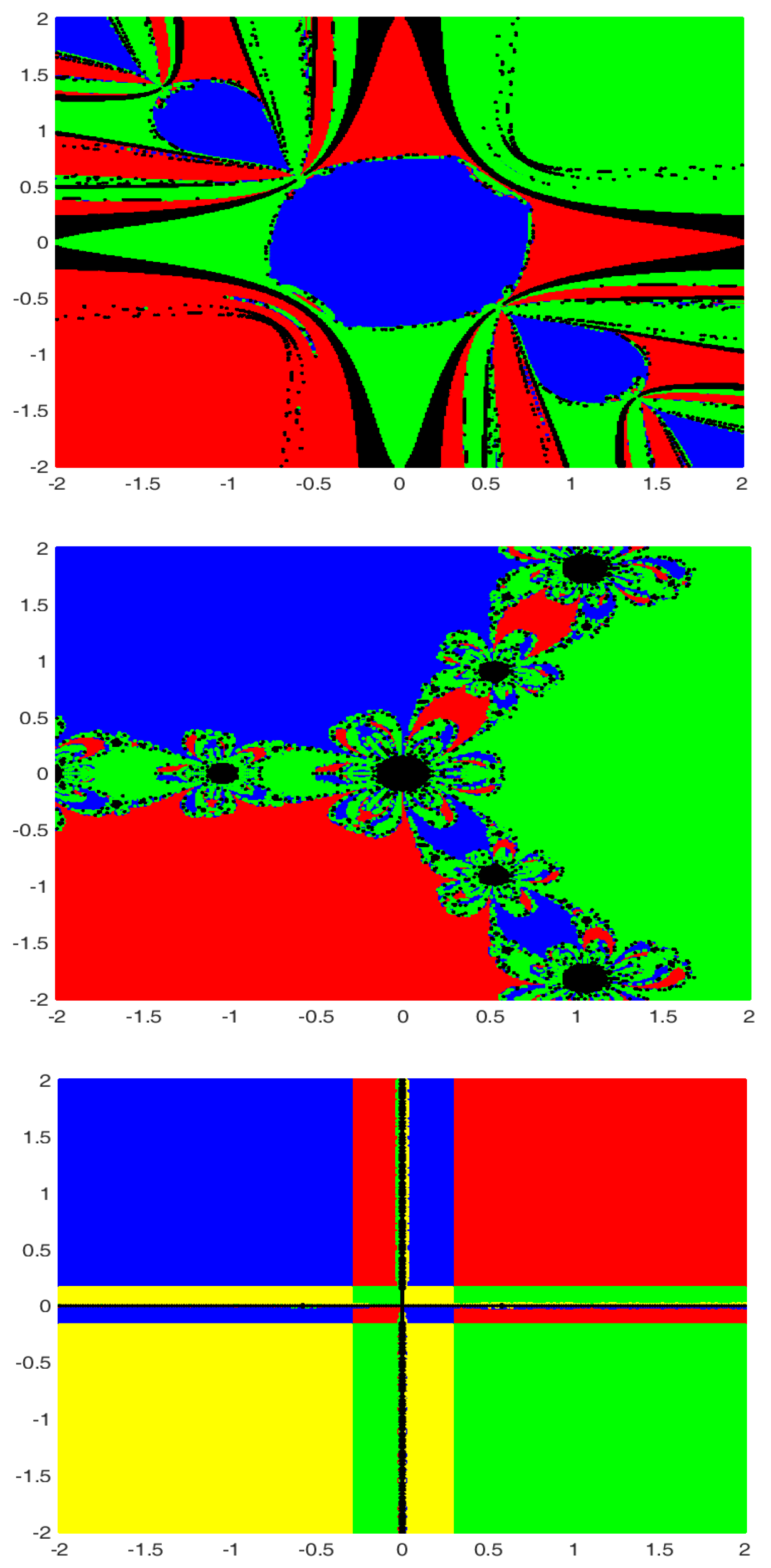
4. Basins of Attractions

The Fatou sets or basins of attraction [2,8,9] of method (3) denoted by $\mathcal{F}atos$ is defined as $\mathcal{F}atos=\{x:x$ is an inital point from which (3) converges to a solution of a given equation }. The complement of $\mathcal{F}atos$ is called the Julia set. We consider three problems that are systems of polynomials in two variables and computed $\mathcal{F}atos$, which is associated with each root of the corresponding systems given in Figure 1:

Example 3.

$\left\{\begin{array}{c}{x}^3-y=0\hfill \\ y^3-x=0\hfill \end{array}\right.$

with solutions $\left\{\right(-1,-1),(0,0),(1,1\left)\right\}$.

Example 4.

$\left\{\begin{array}{c}3x^{2}y-y^3=0\hfill \\ x^3-3x{y}^2-1=0\hfill \end{array}\right.$

with solutions $\{(-\frac{1}{2},-\frac{\sqrt{3}}{2}),(-\frac{1}{2},\frac{\sqrt{3}}{2}),(1,0)\}$.

Example 5.

$\left\{\begin{array}{c}{x}^2+y^2-4=0\hfill \\ 3x^2+7y^2-16=0\hfill \end{array}\right.$

with solutions $\{(\sqrt{3},1),(-\sqrt{3},1),(\sqrt{3},-1),(-\sqrt{3},-1)\}$.

For each test problem, we chose $a=0.3939$ to compute $\mathcal{F}atos$ and compute their dynamics. For this, we consider the region $\mathcal{R}=\{(x,y)\in {\mathbb{R}}^2:x\in [-2,2],y\in [-2,2]\}.$ We make sure that $\mathcal{R}$ contains all the roots of the test problems considered. An equspaced grid of $401\times 401$ points in $\mathcal{R}$ is considered to be the initial guess $X_0$ for the scheme (3). The scheme is iterated to a maximum of 50 iterations with a fixed tolerance of ${10}^{-8}.$ An iterative scheme with initial guess $X_0$ does not converge to any of the roots if the above accuracy is not achieved within 50 iterations, and we assigned black colors to those points $X_0.$ In this manner, we distinguish $\mathcal{F}atos$ by their respective colors for the distinct roots of each method.

Figure 1 demonstrates $\mathcal{F}atos$ corresponding to each root of the method (3). The black region denotes the Julia set.

The figures presented in this work is performed in a 4-core 64 bit Windows machine with Intel Core i7-3770 processor using MATLAB programming language.

5. Conclusions

The local convergence and the dynamics of the Traub method (3) have been studied under weaker-than-before conditions. The technique used allows the extension of the usage of the Traub method to include equations with operators that are less than five-times Fréchet-differentiable. The new technique does not depend on the method. Thus, it can be used on other methods [1,4,7,9].

References

1. Ortega, J.M.; Rheinboldt, W.C. Iterative Solution of Nonlinear Equations in Several Variables, Volume 30 of Classics in Applied Mathematics; Society for Industrial and Applied Mathematics (SIAM): Philadelphia, PA, USA, 2000. [Google Scholar]
2. Argyros, I.K. Unified Convergence Criteria for Iterative Banach Space Valued Methods with Applications. Mathematics 2021, 9, 1942. [Google Scholar] [CrossRef]
3. Argyros, I.K. The Theory and Applications of Iteration Methods, 2nd ed.; Engineering Series; CRC Press: Boca Raton, FL, USA; Taylor and Francis Group: Abingdon, UK, 2022. [Google Scholar]
4. Ostrowski, A.M. Solution of Equations and Systems of Equations, 2nd ed.; Pure and Applied Mathematics; Academic Press: New York, NY, USA; London, UK, 1966; Volume 9. [Google Scholar]
5. Amat, S.; Busquier, S.; Bermudez, C.; Plaza, S. On two families of high order Newton type methods. Appl. Math. Lett. 2012, 25, 2209–2222. [Google Scholar] [CrossRef]
6. Magréñan, A.A.; Gutiérrez, J.M. Real dynamics for damped Newton’s method applied to cubic polynomials. J. Comput. Appl. Math. 2015, 275, 527–538. [Google Scholar] [CrossRef]
7. Behl, R.; Maroju, P.; Martinez, E.; Singh, S. A study of the local convergence of a fifth order iterative method. Indian J. Pure Appl. Math. 2020, 51, 439–455. [Google Scholar]
8. Petković, M.S.; Neta, B.; Petković, L.D.; Dzunić, J. Multipoint methods for solving nonlinear equations: A survey. Appl. Math. Comput. 2014, 226, 635–660. [Google Scholar] [CrossRef]
9. Traub, J.F. Iterative Methods for the Solution of Equations; Prentice Hall: Hoboken, NJ, USA, 1964. [Google Scholar]
Figure 1. F a t o s and Julia set for Examples 3–5.
Foundations 02 00042 g001
Publisher’s Note: MDPI stays neutral with regard to jurisdictional claims in published maps and institutional affiliations.