Abstract
In this paper, we consider the application of brute force computational techniques (BFCTs) for solving computational problems in mathematical analysis and matrix algebra in a floating-point computing environment. These techniques include, among others, simple matrix computations and the analysis of graphs of functions. Since BFCTs are based on matrix calculations, the program system MATLAB® is suitable for their computer realization. The computations in this paper are completed in double precision floating-point arithmetic, obeying the 2019 IEEE Standard for binary floating-point calculations. One of the aims of this paper is to analyze cases where popular algorithms and software fail to produce correct answers, failing to alert the user. In real-time control applications, this may have catastrophic consequences with heavy material damage and human casualties. It is known, or suspected, that a number of man-made catastrophes such as the Dharhan accident (1991), Ariane 5 launch failure (1996), Boeing 737 Max tragedies (2018, 2019) and others are due to errors in the computer software and hardware. Another application of BFCTs is finding good initial guesses for known computational algorithms. Sometimes, simple and relatively fast BFCTs are useful tools in solving computational problems correctly and in real time. Among particular problems considered are the genuine addition of machine numbers, numerically stable computations, finding minimums of arrays, the minimization of functions, solving finite equations, integration and differentiation, computing condensed and canonical forms of matrices and clarifying the concepts of the least squares method in the light of the conflict remainders vs. errors. Usually, BFCTs are applied under the user’s supervision, which is not possible in the automatic implementation of computational methods. To implement BFCTs automatically is a challenging problem in the area of artificial intelligence and of mathematical artificial intelligence in particular. BFCTs allow to reveal the underlying arithmetic in the performance of computational algorithms. Last but not least, this paper has tutorial value, as computational algorithms and mathematical software are often taught without considering the properties of computational algorithms and machine arithmetic.
1. Introduction and Notation
1.1. Preliminaries
In the last 300 years, sophisticated computational algorithms have been developed to solve a wide variety of problems in the mathematical and engineering sciences [1,2,3,4,5]. With the advent of digital computers in the mid-20th century, it became evident that some historical algorithms are unsuitable for direct computer implementation without significant modifications. Meanwhile, other algorithms, despite their cleverness, became obsolete. Consequently, paradigms in scientific computation have evolved, resulting in the creation and deployment of novel computational algorithms as computer codes.
When implemented as computer codes in floating-point computer environment, such as the one realized in the program systems MATLAB® [6,7] and Octave [8], some of these computational algorithms may produce wrong results without warning. In such cases, BFCTs may give acceptable results. BFCTs may also reveal flaws in symbolic codes such as sym(x,′e′) from [6].
Other computer systems, such as Maple [9] and Mathematica [10,11], use variable precision arithmetic to potentially avoid these pitfalls. However, this may lead to an increase in the time required for algorithm performance. In such cases, BFCTs and a detailed analysis of computational problems with reference solution may be useful.
To evaluate and improve BFCTs’ scalability, optimization or parallelization strategies can be employed on larger datasets and higher-dimensional problems. Techniques such as parallel computing, CPU acceleration [12,13], and cloud computing [14] are particularly advantageous. This seems to be a new and challenging research area.
BFCTs may also be used to obtain initial guesses for computational algorithms intended to solve finite equations and minimize functions of one or several scalar arguments. We stress finally that Monte Carlo algorithms [15] are also a form of BFCT. As a perspective, a combination of artificial intelligence [16,17] with BFCTs is yet to be developed.
The computations in this paper are performed using double precision binary floating-point arithmetic obeying the IEEE Standard [18]. Some of the matrix notations used are inspired by the language of MATLAB®. Some of the codes for numerical experiments are given so the results can be independently checked. We finally stress that sometimes, BFCTs reveal the underlying machine arithmetic of the used computing environment.
1.2. General Notations
Next, we use the following general notations.
- —set of integers;
- —set of integers , where ;
- —set of integers ;
- —set of real (complex) numbers;
- —imaginary unit, where ;
- —sum of the scalar quantities ;
- —definite integral of the function on the interval ;
- ≺—lexicographical order on the set of pairs defined as if , or and ; we write if , or ;
- —set of matrices A with elements , where is one of the sets , or ;
- ;
- —pth row of ;
- —qth column of ;
- —spectral norm in ;
- —matrix with unit elements;
- —rank of the matrix ;
- —trace of the matrix ;
- —determinant of the matrix ;
- —identity matrix with and for ;
- —matrix with unique nonzero element, equal to 1, in position ;
- —nilpotent matrix with and for ;
- —eigenvalues of the matrix , where ; we usually assume that ;
- —singular values of the matrix , where , ; the singular values are ordered as ;
- —spectral norm of the matrix ;
- —condition number of the non-singular matrix .
1.3. Machine Arithmetic Notations
We use the following notations from binary floating-point arithmetic, where codes and results in the MATLAB® environment are written in typewriter font.
- —set of finite positive (negative) machine numbers;
- —set of finite machine numbers;
- —rounded value of ; is computed as by the command sym(x,’f’), where , and m is odd if ;
- —set of positive (negative) machine numbers; we have ;
- ()—machine number right (left) nearest to ; is obtained as X + eps(X);
- —machine epsilon; we have , ; is obtained as eps(1), or simply as eps;
- —rounding unit;
- —maximal integer such that positive integers are machine numbers; we have , ;
- —maximal machine integer degree of 2; we have ;
- —maximal machine number; it is also denoted as realmax and we have eps(realmax) = 2^971;
- —minimal positive normal machine number; it is also denoted as realmin;
- —minimal positive subnormal machine number; it is found as eps(0);
- —rounded value of ;
- —normal range; numbers are rounded with relative error less than ;
- Inf (-Inf)—positive (negative) machine infinity;
- NaN—result of mathematically undefined operation, representing Not a Number;
- —extended machine set.
1.4. Software and Hardware
The computations were conducted with the program system MATLAB®, Version 9.9 (R2020b), on a Lenovo X1 Carbon 7th Generation Ultrabook, Memory: 16 GB DDR4 2133 Mhz (2 × 8 GB DIMMs), Video: Intel HD 620, Wholesale China Products, Lenovo Laptop Manifacturer.
1.5. Problems with Reference Solution
An effective strategy for employing BFCTs involves solving CPRSs. CPRSs are specially designed computational problems with a priori known, or reference, solutions. It is supposed that the numerical algorithm which is to be checked does not “know” this fact and solves the computational problem in the standard way. Consider, for example, the finite equation , where and x are scalars or vectors. Then, a CPRS is obtained choosing , where is the reference solution. We usually choose to be a vector with unit elements, e.g., x_ref = ones(n,1) and .
Let be a solution of the equation and be an approximate solution computed in FPA. The relative error of the computed solution depends on the rounding of initial data and on errors made during the computational procedure [19,20]. To eliminate the effects of rounding initial data, we may consider CPRSs with relatively small integer data, or more generally, with data consisting of machine numbers.
Example 1.
Computational algorithms and software for solving linear algebraic equations , where the matrix is invertible, may be checked choosing and , where x_ref = ones(n,1). The computed solution is x_comp = A\b and we may compare the relative error
with the a priori error estimate eps∗cond(A).
Example 2.
Let be a differentiable highly oscillating function with derivative . The numerical integration of may be a problem. For such integrands, we may formulate a numerically difficult computational problem with reference solution . Systems with mathematical intelligence such as MATLAB® [6], Maple [9] and Mathematica [10,11] may find the integral with high accuracy by the NLF , thus avoiding numerical integration.
Example 3.
To check the codes for eigenstructure analysis of a matrix , one can select , where are integer matrices with . The eigenvalues of A are equal to 1 (the reference solution). Computational algorithms such as the QR algorithm and software for spectral matrix analysis may produce wrong results even for matrices of moderate norm.
Example 4.
When solving the differential equation with initial condition , we may choose a reference solution as follows. The function satisfies the differential equation , where
with initial condition .
An important observation is that for some computational problems such as integration and finding the extrema of functions, BFCTs may produce better results than certain sophisticated algorithms used in modern computer systems for calculating mathematics; see, e.g., Section 7.
2. Machine Arithmetic
2.1. Preliminaries
In this section, we consider computations in FPA obeying the IEEE Standard [18]. Numerical computations in MATLAB® are calculated according to this standard. The FPA consists of a set of machine numbers and rules for performing operations, e.g., addition/subtraction, multiplication/division, exponentiation, etc. Rounding and arithmetic operations in FPA are performed with an RRE of order . The sum and the product are computed as and .
A major source of errors in computations is the (catastrophic) cancellation when relatively exact close numbers are subtracted so that the information coded in their left-most digits is lost [21]. Thus, catastrophic cancellation is the phenomenon when subtracting good approximations to close numbers may cause a bad approximation to their difference. Less known is that genuine addition in FPA may also cause large and even unlimited errors.
A tutorial example of cancellation is solving quadratic equations , . During the last 4000 years, students are taught to use the formula , , without warning that this may be a bad way to solve numerically quadratic equations. Similar considerations are valid for the use of explicit expressions for solving cubic and quartic algebraic equations. Genuine subtraction is numerically dangerous, and genuine addition in FPA is not less dangerous, although this fact is not very well known.
2.2. Violation of Arithmetic Laws
In FPA, the commutative law for addition and multiplication is valid, but the associative law for these operations is violated, i.e., it may happen that
The distributive law is also violated. This may lead to unexpectedly large (in fact, arbitrarily large) errors.
For example, we have an incorrect result . The reason for this machine calculation is that is not a machine number (this is the smallest positive integer with this property). It lies in the middle of the successive machine numbers R and and is rounded to R. At the same time, we have , which is the correct answer. Thus, we obtained the famous wrong equality arising in mathematical jokes.
This is not the end of the story. Consider the expression consisting of members, where there are R members equal to 1. We have . Computing S from left to right, we obtain the wrong answer . Computing S starting with the ones, i.e., we obtain the correct answer . Now, we have obtained the more impressive result . Summing (at least theoretically) a sufficient number of 1s, we compute the sum as Inf and hence (note that the summation of arbitrarily large number of collectibles is not a problem for Turing-Post machines).
The associative law for multiplication is also violated in FPA. For example, the value of the expression is and it is computed correctly as
At the same time, the machine computation of P from left to right gives
where is the symbol for infinity in FPA. Thus, we obtained .
Similar false equalities are obtained by the addition and subtraction of a small number of machine numbers. Set . In standard arithmetic, we have . In FPA, it is fulfilled . This corresponds to the wrong equality although E is a machine number at a good distance to .
We also have , although the exact result is and should be rounded to -Inf. Thus, we obtained . The reason is that the maximum positive machine number in FPA is and the number is set to . Moreover, the maximum positive integer that is still rounded to is while the number is set to Inf.
These entertaining exercises may produce undetermined results as well. For example, we have but the computed value is U = Inf/Inf − 1 = NaN. This may be interpreted as the exotic equality .
Working with positive numbers also leads to violation of the distributive law . In particular, we usually think that for , it is fulfilled . But setting , we obtain (x + x)/2 = 2∗x/2 = x and x/2 + x/2 = 0 + 0 = 0. We stress that the minimal positive quantity that is still rounded to instead to 0 is .
The distributive law in the form (1/m + 1/n)/p = 1/m/p + 1/n/p, where at least one of the operands is not an integer degree of 2, is also violated. In this case, the rounded values of both sides of the equality are usually neighboring machine numbers.
Example 5.
Let , , . Then, and .
Example 5 shows that the machine subtraction of close numbers is usually performed with a small relative error. Moreover, if the operands are machine numbers and , then the machine subtraction is exact [21].
The rounded value of is computed by the command sym(X,’f’) in the form , where and m is odd when . In particular, the command sym(realmax,’f’) will give 309 decimal digits of the integer = realmax.
2.3. Numerical Convergence of Series
We shall conclude our brief excursion in the machine summation of numbers with the consideration of numerical series with positive elements . For , set .
Definition 1.
The symbol is called a numerical series. The quantity is the n-th partial sum of this series.
The partial sums are computed in FPA as , , . Theoretically, the series is divergent when . In FPA, there are three mutually disjoint possibilities according to the next definition.
Definition 2.
The series adheres to the following:
- 1.
- Numerically convergent if there is a positive and such that for ; the number S is called the numerical sum of the series ;
- 2.
- Numerically divergent if there is such that for ; in such cases, for ;
- 3.
- Numerically undefined if there is such that for and .
Divergent numerical series may be numerically convergent. For example, the divergent harmonic series with is numerically convergent in FPA to a sum . The divergent series with is numerically convergent to . Also, it is easy to prove the following assertion.
Proposition 1.
For any there is a series which is numerically convergent to S.
Proposition 1 for FPA is an analogue to the Riemann series theorem [22], which states that the members of a convergent real series which is not absolutely convergent may be reordered so that the sum of the new series is equal to any prescribed real number.
2.4. Average Rounding Errors
We recall that the normal range of FPA is the interval such that numbers are rounded with an RRE less than .
Let and be the rounded value of x. It is well known [18] that the RRE satisfies the estimate
The code sym(x,’f’) computes in the form , where is odd if . Let . The expression between two successive machine numbers
in the interval is as follows. Let
Then,
The maximum value of in the interval is achieved for and is equal to
A part of the graph of the function is shown in Figure 1.
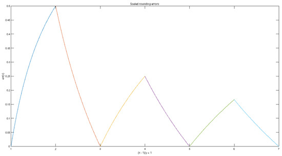
Figure 1.
Scaled rounding errors.
For near to , the maximum RRE is about , while for near to , the maximum RRE is close to . In particular, we have
That actual behavior of RRE is not governed by (1) but is considerably smaller and has been known to specialists in computer calculations for a long time. To clarify this problem, we performed intensive numerical experiments.
BFCTs showed that the actual RRE is considerably lower than and this led to the definition and use of average RREs, which are more realistic in comparison to the relative error . Based on this observation [23], we have defined and calculated an integral ARRE as the definite integral . This integral is of order
At the same time, the average of the RRE maximums is
Intensive numerical BFCT experiments [23] with the rounding of large sequences of numbers had shown that the actual ARRE is about . This is 2.5 times less than the widely used bound in the literature [18]. In these experiments, numbers had been excluded, because . This explains why the multiplier of was computed as 0.40 instead of 0.35.
In another experiment, we have computed and averaged the RRE for fractions , and for and m up to 1000, and we have computed the ratios . The results are shown in Table 1. The actual RRE in rounding of unit fraction (second column) is very close to the integral ARRE (3).

Table 1.
Ratios for certain fractions.
For fractions close to 1, the computed ARRE is larger than for fractions close to 2. This confirms the observation that the rounding of , , is made with a lower (although not twice as low) RRE for x close to the left limit compared with close to the right limit of the interval; see (2). For example, the result in cell (4, 2) of Table 1 is obtained by the code
for m = 1:1000
R(m) = double(abs((sym(1/m,’e’)−1/m))∗m∗2/eps);
end
mean(R)
We stress that in such experiments, we cannot use pseudo-random number generators such as rand, randn and randi from MATLAB® since they produce machine numbers for which the rounding errors are zero.
We summarize the above considerations in the next important proposition.
Proposition 2.
The known rounding error bounds in all computational algorithms realized in FPA may be reduced three times (!) if the integral ARREs are used instead of the maximum RRE.
It must be pointed out that some widely used computer codes for evaluation of the rounding process have serious flaws. The MATLAB® code sym(x,’e’) should compute the rounded value of in the form with signed absolute rounding error . However, for and , the value of is computed with a relative error of almost 100%.
3. Numerically Stable Computations
3.1. Lipschitz Continuous Problems
The numerical stability of computational procedures is a major issue in numerical analysis [19]. A large variety of computational problems (actually, almost all computational problems) may be formulated as follows; see [19,20]. Let and be given sets and let be a continuous function. We shall use the following informal definition.
Definition 3.
The computational problem is described by the function f, while the particular way of computing the result for a given data is the computational algorithm.
Thus, the computational problem is identified with the pair , or with the equality . For many computational problems, the function f is Lipschitz continuous.
Definition 4.
The computational problem is said to be (locally) Lipschitz continuous if there exist constants and such that
whenever . The problem is globally Lipschitz continuous if .
If the function f has a locally bounded derivative, it is (locally) Lipschitz continuous. The concept of Lipschitz continuity is illustrated by the next example.
Example 6.
Let , , and be a given constant. Then, the following assertions take place.
- 1.
- The function is Lipschitz continuous if and is not Lipschitz continuous if .
- 2.
- The function is Lipschitz continuous if and is not Lipschitz continuous if .
- 3.
- The function , , is Lipschitz continuous if and is not Lipschitz continuous if .
- 4.
- The function for and , is differentiable on but is not Lipschitz continuous.
Suppose now that the algorithm is realized in FPA, e.g., in the MATLAB® computing environment.
Definition 5.
The computational algorithm is said to be numerically stable if the computed result is close to the result of a close problem with data .
Definition 5 includes the popular concepts of forward and backwards numerical stability. To make this definition formal, suppose that there exist non-negative constants such that
and , . Further on, we have
Dividing the last inequality by , we obtain the following estimate for the relative error in the computed solution
Definition 6.
The quantity is said to be the relative condition number of the computational problem .
The remarkable Formula (4) reveals the three main factors that determine the precision of the calculated solution [20,23].
Proposition 3.
The precision of the computed solution depends on the following factors.
- 1.
- The sensitivity of the computational problem to perturbations in the data d measured by the Lipschitz constant L of the function f.
- 2.
- The stability of the computational algorithm expressed by the constants .
- 3.
- The FPA characterized by the rounding unit ρ and the requirement that the intermediate computed results belong to the normal range .
The error estimate (4) is used in practice as follows. For a number of problems, the Lipschitz constant L may be calculated or estimated as in the solution of linear algebraic equations and the computation of the eigenstructure of a matrix with simple eigenvalues. Finally, the value of is known exactly for FPA as well as for other machine environments.
Estimation of the constants may be a problem. Often, the heuristic assumption and is made giving
It follows from (5) that C will be large if L and/or are large and/or is small. The constant L is usually outside the user’s control. The quantities and may be changed by scaling of the computational problem.
Definition 7.
The computational problem is said to adhere to the following:
- 1.
- Well conditioned if ; in this case, we may expect about true decimal digits in the computed solution;
- 2.
- Poorly conditioned if ; in this case, there may be no true digits in the computed solution.
More precise classification of the conditioning (well, medium and poor) of computational problems is also possible. Computational problems that are not Lipschitz but Hölder continuous may also be analyzed: see, e.g., [23].
The above considerations confirm a fundamental rule in numerical computations, namely that if the data d and/or some of the intermediate results in the computation of are large and/or the result is small, then large relative errors in the computed solution can be expected; see Section 3.3. For some computational problems , there are a priory error estimates for the relative error in the computed solution in the form of explicit expressions in and d. The importance of such estimates is that they may be obtained a priori before solving the computational problem.
Most a priory error estimates are heuristic. Among computational problems with such estimates is the solution of linear algebraic equations and the computation of the eigenvalues of a matrix A with simple spectrum. To check the accuracy and practical usefulness of such error estimates by BFCTs, a set of CPRSs is designed, and the error estimates are compared with the observed errors.
3.2. Hölder Continuous Problems
Definition 8.
The computational problem is said to be Hölder continuous with exponent if there exist constants and such that
whenever .
Hölder continuity implies uniform continuity, but the converse is not true. It is supposed that . Indeed, if , the problem is Lipschitz continuous, and if , the function f is constant.
The machine computation of may be performed with large errors of order when the exponent is small. Such cases arise in the calculation of a multiple zero of a smooth function , where , and . In this case, .
Let and be the computed value of r. Then, a heuristic accuracy estimate for the solution of a Hölder problem is
Experimental results confirming this estimate are presented later on. A typical example of a Hölder problem is the computation of the roots of an algebraic equation of n degree with multiple roots, where (the case is treated by special algorithms). There are three codes in MATLAB® that can be used for solving algebraic equations which may be characterized as follows.
- The code roots is fast and works on middle power computer platforms with equations of degree n up to several thousands but gives large errors in case of multiple roots. This code solves only algebraic equations.
- The code vpasolve works with VPA corresponding to 32 true decimal digits with equations of degree n up to several hundreds but may be slow in some cases. This code works with general equations as well finding one root at a time.
- The code fzero is fast but finds one root at a time. It may not work properly in case of multiple roots of even multiplicity. This code works with general finite equations as well.
3.3. Golden Rule of Computations
The results presented in this and previous sections confirm the golden rule of computing both exact and machine arithmetic, which may be formulated as follows.
Proposition 4 (Golden Rule of Computations).
If in a chain of numerical computations the final result is small relative to the initial data and/or to the intermediate results, then large relative errors in the computed solution are to be expected.
Note that the already mentioned catastrophic cancellation in subtraction of close numbers is a particular case of Proposition 4.
An important class of computations in FPA are the so-called computations with maximum accuracy. Let the vector r with elements be the exact solution of the vector computational problem and let the vector with elements be the computed solution.
Definition 9.
The vector is computed with maximum accuracy if its elements satisfy .
Solutions with maximum accuracy are the best that we may expect from a computational algorithm implemented in FPA.
4. Extremal Elements of Arrays
Finding minimal and maximal elements of real and complex arrays is a part of many computational algorithms. This problem may look simple, but it has pitfalls in some cases.
4.1. Vectors
Let be a given real n-vector. The problem of determining an extremal (minimal or maximal) element of w together with its index k arises as part of many computational problems. The solution of this problem is obtained in MATLAB® by the codes [U,K] = min(w) and [V,L] = max(w), where is the minimal element of the vector w and K is its index. Similarly, is the maximal element of the vector w and L is its index. These codes work for complex vectors as well if the complex numbers are ordered lexicographically by the relation ⪯; see [6].
An important rule here is that if there are several elements of w equal to its minimal element U, then the computed index K is supposed to be the minimal one. Similarly, if there are several elements of w equal to its maximal element V, then the computed index L is again the minimal one. The delicate point here is the calculation of the indexes K and L. For example, for , where or , the codes min and max produce , and , as expected.
Due to rounding, the above codes may produce unexpected results. Indeed, the performance of the codes depends on the form in which the elements of the vector w are written.
Example 7.
The quantities , and are equal but their rounded values are different. The rounded value of is computed by the code sym(X,’f’) . It produces the answer in the form , where . We have and , . Hence, .
Example 8.
Let w be a 3-vector with elements at any positions, where are defined in Example 7. Then, the code [U,K] = min(w) will give and K will be the index of B as an element of w. The code [V,L] = max(w) will give and L will be the index of C as an element of w. At the same time, both codes are supposed to give and .
These details of the performance of the codes min and max may not be very popular even among experienced users of sophisticated computer systems for mathematical calculations such as MATLAB®.
4.2. Matrices
Similar problems as in Section 4.1 arise in finding extremal (minimal or maximal) elements of multidimensional arrays and in particular of real and complex matrices A.
Consider a matrix with elements . Let the minimal element of A relative to the lexicographical order be . Then, the code
[a,b] = min(A); [A_min,N] = min(a); A_min, ind = [b(N),N]
finds the minimal element of A and the pair of its indexes as
A_min, ind = i_1 i_2
where i_1 = ind(1), i_2 = ind(2). Here, a and b are n-vectors and ind is a 2-vector.
If there is more than one minimal element, then the computed pair of its indexes is minimal relative to the lexicographical order. This result, however, may depend on the way the elements of A are specified.
Finding minimal elements of matrices may be a part of improved algorithms to compute the extrema of functions of two variables; see Section 7.2. A scheme for finding minimal elements of -arrays, , may also be derived and applied to the minimization of functions of n variables.
4.3. Application to Voting Theory
The above details in using the codes min and max from MATLAB® [6], although usually neglected, may be important. For example, in certain automatic voting computations (in which one of the authors of this paper had participated back in 2013) with the Hamilton method for the bi-proportional voting system used in Bulgaria, these phenomena actually occurred and caused problems. To resolve quickly the problem, we applied BFCTs using hand calculations (!) being in an emergency situation.
The computational algorithms for realization of the Hamilton method must be improved, replacing the fractional remainders by integer remainders [23] as follows. Let n parties with votes take part in the distribution of parliamentary seats by the Hamilton method [24]. Set and .
Next, the rationals are represented as , where is the integer part of , is the fractional remainder and is the integer remainder of modulo V. Initially, the kth party obtains seats. If the sum of initial seats is less than S, then the first parties with largest integer remainders obtain one seat more. Thus, to avoid small errors in the computation of fractional remainders that may cheat the code max, we must work with exactly computed integer remainders .
5. Problems with Reference Solutions
5.1. Evaluation of Functions
Evaluation of functions f defined by an explicit expression
is a CPRS, since may be found with high precision in a suitable computing environment. However, the relative error in computing y may be large even for well-behaved functions f and arguments x far from the limits of the normal range [23]. The reason is that instead with the argument , the corresponding computational algorithm works with the rounded value . At the same time, for , the computed quantity is usually exact to working precision.
Example 9.
We have
[cos(realmax);sin(realmax)] = −0.999987689426560
0.004961954789184
The computed result is correct to full precision, although the argument realmax is written with 309 decimal digits, which may be displayed by the command sym(realmax,’f’).
Let the function f be locally Lipschitz continuous with constant in a neighborhood of x and let the result computed in FPA be . Then, the relative error of is estimated as
where is the relative condition number of the computational problem .
Example 10.
Consider the vector , where . We should have but for large k, this may not be so. Let the vector have elements , i.e.,
X = pi∗[2^47,2^48,2^49,2^50,2^51,2^52,2^53,2^54]
The command Y = [cos(X);sin(X)] gives the matrix
Y = 0.9999 0.9994 0.9976 0.9905 0.9622 0.8517 0.4509 −0.5934
0.0172 −0.0345 −0.0689 −0.1374 −0.2723 −0.5240 −0.8926 −0.8049
While the first column Y(:,1) of Y still resembles the exact vector [1;0], the next columns are heavily wrong with Y(:,8) being a complete catastrophe with relative error 170%. The commands Y1 = [C1;S1] and Y2 = [C2;S2], where C1 = vpa(cos(X)), S1 = vpa(sin(X)), C2 = cos(vpa(X)) and S2 = sin(vpa(X)) produce the same wrong result Y1 = Y2 = Y.
The reader is advised to plot the graph of the eight functions , , by the command syms x; fplot(sin(x+X)), for the vector X from Example 10. A way out from such wrong calculations is to evaluate standard -periodic trigonometric functions for arguments modulo .
Example 11.
The command
YY = [cos(mod(X,2∗pi));sin(mod(X,2∗pi))]
produces the matrix
YY = 1 1 1 1 1 1 1 1
0 0 0 0 0 0 0 0
which is exact to full precision.
We recall that for , the rounded value of x is an even integer. For example, the quantity is rounded to , which is demonstrated by the command sym(23∗pi^32/20,’f’). Another instructive example is rounding integer decimal degrees .
Example 12.
We have for but
sym([10^23;10^24;10^25],’f’) = 99999999999999991611392
999999999999999983222784
10000000000000000905969664
If , then for most elementary and special functions f, the quantity is computed with maximum accuracy.
If the function f is locally Lipschitz with constant , then large relative computational errors in the evaluation of may occur when is large, i.e., when and/or is large and/or is small. For the trigonometric functions above the quantities, and are equal to 1, but the argument is large.
A standard approach to improve the performance of computational algorithms is to scale the initial and/or intermediate data to avoid large errors. In computing the matrix exponential , , the scaling is accomplished by a scaling factor , , which is a binary degree in order to reduce rounding errors [19].
5.2. Linear Algebraic Equations
An instructive example, which illustrates BFCTs to the solution of vector algebraic equations with integer data, is designed as follows. Let be invertible matrix and . The command A = fix(100∗randn(n)) generates a matrix that is normally distributed with integer elements of moderate magnitude and zero mean (similar effect is achieved by the command randi). Choosing the reference solution as X_0 = ones(n,1), we obtain b = A∗X_0. The computed solution is X_comp = A\b with relative error E_n = norm(X_comp − X_0)/sqrt(n).
The a priori relative error estimate is est = eps∗cond(A). Usually, is a small multiple of , and this may be checked by BFCTs. We consider three types of computed solutions as follows.
- Standard solution X_1 = A\b obtained by Gaussian elimination with partial pivoting based on LR decomposition of A, where L is a lower triangular matrix with unit diagonal elements, R is an upper triangular matrix with nonzero diagonal elements, and P is a permutation matrix.
- Solution X_2 = R\(Q’∗b) obtained by QR decomposition [Q,R] = qr(A) of A, where , the matrix Q is orthogonal and the matrix R is upper triangular.
- Solution X_3 = inv(A)∗b based on finding the inverse of A.
The solution is computed as a default in MATLAB® and is accurate and fast. The solution is very accurate although more expensive and is also used. The solution is not recommended and is included here for tutorial purposes. Indeed, computing inv(A) and multiplying the vector b by this matrix are unnecessary operations which are expensive and reduce accuracy.
The above computational techniques are illustrated by the commands
n = 1000; A = fix(100∗randn(n)); X_0 = ones(n); b = A∗X_0;…
X_1 = A\b; [Q,R] = qr(A); X_2 = R\(Q’∗b); X_3 = inv(A)∗b;…
E_1 = norm(X_0-X_1)/sqrt(n);E_2 = norm(X_0-X_2)/sqrt(n);…
E_3 = norm(X_0-X_3)/sqrt(n);est = eps∗cond(A);…
e_1 = E_1/est; e_2 = E_2/est; e_3 = E_3/est; [e_1;e_2;e_3]
Each execution of these commands produces different results because of the code randn. The computed quantity e_1 for systems with up to unknowns is usually less than 20, the quantity e_2 is about 40 and the quantity e_3 is less than 4. More precisely, intensive computations with showed that , and .
Tests with had also been conducted, but they require more computational time. For such values of n, we have observed average values , , and .
The comparison of and with confirms, among others, the tutorial conclusion that solving linear vector algebraic equations by matrix inversion must definitely be avoided. Rather, the opposite is true. If the inverse matrix is needed for some reason, it is found solving n equations for the columns of B, where is the kth column of .
Our main observation, based on BFCTs, featuring a comparison of the methods of Gaussian elimination and QR decomposition for solving linear algebraic equations, is formulated in the next proposition.
Proposition 5.
For matrices of order up to 1000, the QR decomposition method gives a relative error that is between 5 and 10 times less than the relative error of the Gaussian elimination method.
In addition, the solution of the equation via QR decomposition is backward stable, which is not always the case with Gaussian elimination with partial pivoting. Thus, Proposition 5 is a message to the developers of mathematical software such as MATLAB®.
The Gaussian elimination method based on LR decomposition is preferred to the QR decomposition method because it requires half the floating-point operations. Since fast computational platforms are now widely available, this consideration is no longer valid.
Although the implementation of the code x = A\b gives good results for matrices with n of order up to 1000, large errors in x may occur even for in some cases.
Example 13.
Consider the algebraic equation , where the matrices are defined by the relation (7) below. For , we have . The computed results for are presented in Table 2. In cases , there is a warning that the matrix is close to singular or badly scaled, since is larger than . As shown in Table 2, for these two cases, the relative error is indeed 25% and 100%, respectively.
Table 2.
Errors and estimates for low order systems.
5.3. Eigenvalues of 2 by 2 Integer Matrices
The integer matrix
with condition number has double eigenvalue and Jordan form . The elements of A are integers of magnitude . This is far from the quantity such that integers may not be machine numbers.
Example 14.
The MATLAB® code e = eig(A) computes the column 2-vector e of eigenvalues of A as instead of . The relative error is 140%, and there is no true digit in the computed vector (even the sign of the first computed eigenvalue is wrong). The trace of A is fortunately computed as trace(A) = 2 and is the sum of the wrong eigenvalues. Next, the determinant of A (which is equal to 1) is computed wrongly in MATLAB® as det(A) = 0.2214.
Surprisingly, the vector p of the coefficients of the characteristic polynomial of A, computed as p = poly(A), is [1,−2,−0.9475]. The last element of the vector p has nothing in common with the computed determinant 0.2214, which may further confuse the user. Next, the Schur form of A is computed by the MATLAB® command [U,S] = schur(A) as
and we have . This explains the computed value of .
Finally, we may try to compute as , where represents the singular values of A. Based on the MATLAB® code svd, the computed result is , which is the best approximation to the exact value 1 of the determinant up to now. The same result for is obtained by the QR decomposition of A by the MATLAB® command [Q,R] = qr(A). The above results confirm the rule that SVD and QR decomposition are the best numerical tools to compute the determinant of a general matrix (if this determinant is ever needed). For general matrices, however, the most reliable way to compute the spectrum is a variant of the BFCT described below. Here, we recall the modern paradigm in numerical spectral analysis and root finding of polynomials: the eigenvalues of a matrix are not computed as roots of its characteristic polynomial but rather the contrary: the roots of a polynomial are computed as the eigenvalues of its companion matrix.
The Maple [9] code jordan(A), incorporated in MATLAB®, computes correctly the Jordan form of A. The vector of eigenvalue condition numbers, computed by the MATLAB® command condeig(A), is , where is relatively large. This indicates that something is wrong. In reality, things are even worse, since the 2-vector of eigenvalue condition numbers of the matrix A does not exist because A has only one linearly independent eigenvector. At this moment, the user may or may not be aware that something is wrong (with exception of the code jordan which is not very popular and is of restricted use). Now comes the time of BFCTs to find the spectrum and the Jordan form of A as follows.
The sum of the eigenvalues of A is equal to the trace which is computed exactly. If the eigenvalues are close or equal, because the eigenvalue condition numbers are large, then we should have and . The Jordan form of A is then either or . But the only matrix with Jordan form is itself, and hence the Jordan form of A must be . We have obtained the correct result using BFCTs and simple logical reasoning.
The matrix (6) may be written as
for . Thus, we have a family of matrices parametrized by the integer m. The trace of is equal to 2, the determinant of is equal to 1, the eigenvalues of are and the Jordan form of is .
Below, we give the values of the coefficients and of the characteristic polynomial of A as found by the code poly(A), and of the eigenvalues of A, as computed by the code eig(A) in MATLAB®.
- For , we have , and , where the quantity 1.0000 has at least 5 true decimal digits and is a small imaginary tail which may be neglected. This result seems acceptable.
- For , we have , and , . With certain optimism, these results may also be declared as acceptable.
- For , a computational catastrophe occurs with (true), (completely wrong) and , (also completely wrong). Here, surprisingly, is computed as , which differs from 1 (which is to be expected) but differs also from . It is not clear what and why had happened. Using the computed coefficients , the roots of the characteristic equation now are , instead of the computed and . This is a strange wrong result.
- We give also the results for which are full trash and are served without any warning to the user. We have , and . We also obtain for completeness.
In all cases, the sum of the wrongly computed eigenvalues is almost exact, which is a well known fact in the numerical spectral analysis of matrices [19]. The conclusion from the above considerations is that BFCTs in this case, in contrast to the standard software, always give with five true decimal digits. This is a good approximation to the eigenvalues of the matrices for when the codes eig and poly fail.
The main reason for the large errors considered in this section is the bad conditioning of the integer matrices. Nevertheless, these errors are served without warning to the user. This should stimulate teaching computer methods and algorithms with an emphasis on cases where these tools produce wrong (sometimes completely wrong) results. This may also be a stimulus for producers of scientific software to warn users of the possible unreliable behavior of computer codes. Such behavior may be due to the particularities of FPA obeying the 2019 IEEE Standard but also to inappropriate algorithms and programming flaws such as in the code sym(1/1161,’e’).
6. Zeros of Functions
Computing zeros of functions and of polynomials in particular is a classical problem in numerical analysis. Although powerful computational algorithms for this purpose have been developed, the use of BFCTs in this area is still useful.
Consider first the scalar case. Calculating roots of equations , where is a continuous function, in a given interval , may be a difficult problem. We distinguish three main tasks.
- Find a single particular solution in the interval T.
- Find the general solution in the interval T.
- Find all roots of a given n degree polynomial .
The condition guarantees that there is at least one solution in the interval . Whether f has zeros at the points is checked by direct computation.
Solving real and complex polynomial equations of n degree
is achieved by the code vpasolve(P(x) == 0) from MATLAB®. It finds all roots of with quadrupole precision of 32 true decimal digits. For , the speed of the corresponding software on a medium computer platform is still acceptable. For and higher, the performance of the code may be slow even on fast platforms, and hence it may not be applicable to RTA (if such computations are ever needed in RTA). Note that we write this at the beginning of year 2025.
A faster solution may be obtained by the code roots(p), where p is the vector of coefficients of . This code computes the column vector of roots of as the vector of eigenvalues of the companion matrix of using the QR algorithm, i.e., r = eig(compan(p)). The code roots(p) works relatively fast for n up to several thousands but may produce wrong results even for small values of n when the polynomial has multiple roots and the computational problem is poorly conditioned. BFCTs allow to reveal the behavior of this solver.
It is known that errors in computing multiple roots of equations in FPA, where f has a sufficient number of bounded derivatives around a root , are of order , where n is the multiplicity of r and is a constant. To estimate , consider the equation when the n degree polynomial has n-tuple root . Let
be the relative error in the vector computed by the code roots. The ratio is shown in Table 3 for the extended form of the polynomial and values of n from 3 to 20. For , the computed roots are exact and .
Table 3.
Constants in error estimates for code roots.
The relative error in the computed solution for satisfies the heuristic estimate , where the average of is or approximately . The expanded form of the polynomial may be found by the command expand or asking the intelligent dialogue system WolframAlpha [11] to find the coefficients of this polynomial. We stress that for all n values, the code vpasolve(P(x) == 0) gives the exact solution vector .
Usually, the computed roots are unacceptable if their relative error is greater than 1%. For example, it follows from Table 3 that the root of multiplicity 20 is computed by the code roots with a relative error of 32%, which is unacceptable. It must be stressed that this is not due to program disadvantages but rather to the high sensitivity of the eigenvalues of the companion matrix . If the polynomial equation has a root of multiplicity n, the relative error is estimated as . Solving the inequality , we obtain . We summarize these slightly unexpected observations as follows.
Proposition 6.
The errors in computing roots of n-degree polynomials by the code roots may be unacceptable when .
Consider finally the problem of finding all roots of the equation in the interval , i.e., finding the set , where, e.g., , . Here, the use of BFCTs seems necessary. A direct approach is to plot the graph of the function , . Let N be a sufficiently large integer. We may use the commands X = linspace(a,b,N); Y = abs(f(X)); plot(X,Y) to plot the graph of the function , . The zeros of f are now marked as inverted peaks at the roots . In the latter case, we have , and . Next, the codes vpasolve(f,r_k) or fzero(f,r_k) may be used around each of the points to specify the roots with full precision. This approach is well known in the computational practice and is recommended in some MATLAB® guides.
A difficult problem is the solution of nonlinear vector equations and of matrix equations , where x and are n-vectors, and X and are matrices. The MATLAB® code fsolve is intended to solve nonlinear vector equations, while the codes are, axxbc, care, dare, dlyap, dric, lyap, ric, sylv and others solve linear and nonlinear matrix equations. The performance of all these codes may be checked by BFCTs and CPRSs. This a challenging problem which will be considered elsewhere.
7. Minimization of Functions
7.1. Functions of Scalar Argument
The minimization of the expression , , where is a continuous function, is accomplished in MATLAB® by a variant of the method of the golden ratio. The corresponding code [x_0,y_0] = fminbnd(f,a,b) finds a local minimum in the interval T, where . To find the global minimum of f in the interval T, we may use the graph of the function f plotted by the commands x = linspace(a,b,n); y = f(x); plot(x,y). Then, the approximate global minimum of f is determined visually, considering also the pairs and at the end points of T. The code
[x_min,y_min] = fminbnd(f,c-h,c+h)
is then used in a neighborhood of the approximate minimum . This approach requires human interference in the process and may be avoided as shown later.
The problem with the code fminbnd is not that it may find local minimums. The real problem with this and similar codes is that they can miss the global minimum even when the function f is unimodal, i.e., when it has a unique minimum. BFCTs for such functions are a must. The problem is that usually, we do not know whether the function is unimodal or not and whether the computed minimum is minimum at all: the more so when performing complicated algorithms in RTA.
Example 15.
Consider the function
This function is unimodal with minimum . In some cases, this minimum is found as [x_min,y_min] = fminbnd(f,0,b) for some . But in other cases, it is not found correctly, and here, we should use BFCTs. The code works well for but gives a completely wrong result for without warning. Indeed, we have the good result
[x_min;y_min] = fminbnd(f,0,16.85) = 0.999992123678799
1.000000000124073
and the bad result
[x_min;y_min] = fminbnd(f,0,16.86) = 16.859937887512295
2
The second result has a 1586% relative error for and 100% relative error for .
The reason for the disturbing events in Example 15 is complicated. We may expect that for values of x such that the expression is less than since then is rounded to 2. The root of the equation is , and we indeed have . But is much less then 16.86, and hence the code fminbnd works with a certain sophisticated version of VPA instead of with FPA. In particular, the quantity is much less than with . We shall summarize the above considerations in the next statement.
Proposition 7.
The software for the minimization of functions of one variable such as fminbnd(f,a,b) from MATLAB® may fail to produce correct results even for unimodular functions f.
In contrast, BFCTs can always be used to find the global minimum automatically. Let the function be unimodal. Consider the vectors X = linspace(a,b,n+1) with elements and with elements . The MATLAB® command [y,m] = min(Y) computes an approximation to the minimum . Finally, the (almost) exact minimum is computed between the neighboring elements of as [x_min,y_min] = fminbnd(f,X(m−1),X(m+1)). This approach may be used to develop improved versions of the code fminbnd.
7.2. Functions of Vector Argument
For , the minimization of continuous functions of vector argument meets difficulties similar to those described in Section 7.1 and other specific difficulties as well. Unconstraint minimization is accomplished in MATLAB® by the Nelder–Mead algorithm [25,26] and realized by the code fminsearch [6]. We stress that the code finds a local minimizer of the function f, where .
The function f may not be differentiable, which is an advantage of this algorithm. The algorithm compares the function values at the vertexes of an -simplex and then replaces the vertex with the highest value of f by another vertex. The simplex usually (but not always, as shown below) contracts on a minimum of f which may be local or global. The corresponding command is [x_min,y_min] = fminsearch(f,x_0), where is the initial guess. The computed result depends on the next five factors, which include the following:
- The computational problem;
- The computational algorithm;
- The FPA;
- The computer platform;
- The starting point .
Factors 1–3 are usually out of the control of the user. Factor 4 is partially under control, e.g., the user may use another platform. Only factor 5, which is very important, is entirely under control. As mentioned above, the computed value depends on the starting point . This is denoted as .
Definition 10.
The point is said to be a numerical fixed point (NFP) of the computational procedure if .
The computed result is the NFP of the computational procedure. The NFP depends not only on the computational problem and the computational algorithm but also on the FPA and on the particular computer platform where the algorithm is realized. Unfortunately, computed values for which are far from any actual minimum are often NFPs of the computational procedures, and they are served without warning to the user.
For a class of optimization problems, the function f has the form
where , is a polynomial in x and are positive constants. Since , when , the function (8) has (at least one) global minimum .
Numerical experiments with functions f of type (8) show that not only the computed valus for and depend on the initial guess but that in many cases, the code fminsearch produces a wrong solution for which is far from any minimizer of the function f. The reason is that the value of may become very small relative to c. Then, is computed as c, and the algorithm stops at a point which is far from any minimizer of f. Usually, no warning is issued for the user in such cases. This may be a problem when the minimization code is a part of an automatic computational procedure which is not under human supervision. In such cases, application of the techniques of AI and MAI may be useful.
Example 16.
f = @(x)2-x(1)∗x(2)∗exp(1-x(1)^2/2-x(2)^2/2)
The function , , has two global minimizers and for which It also has two global maximizers and for which
Let the initial guess for the code [x_min,y_min] = fminsearch(f,x_0) be . For , we obtain the relatively good result
x_min = −1.000041440968428 −0.999998218805417
y_min = 1.000000001720503
For the slightly different value , the computed result is a numerical fixed point which is not a minimizer. Indeed, we have
x_min = 6.430900000000000 6.430900000000000
y_min = 2.000000000000000
The second computed result in Example 16 is a numerical catastrophe with 543% relative error in and 100% relative error in . The reason is that for and is rounded to 2. The conclusion is that the algorithm of the moving simplex uses FPA rather than VPA (compare with Example 15).
The minimization problem in Example 16 is not unimodal, since it has two solutions. Solving unimodal problems by the code fminsearch may also lead to large errors, as shown in the next example.
Example 17.
f = @(x)2−x(1)∗exp(1/2−x(1)^2/2−(x(2)−1)^2)
The minimization problem has unique solution , . For , the code
[x_min,y_min] = fminsearch(f,[c,c])|
gives a quite acceptable result, namely
x_min = 1.000039724696251 1.000017661431510
y_min = 1.000000001889957
For a slightly different value of c, the computed result is a numerical fixed point which is not a minimizer. Indeed, for , the computed result is wrong, namely
x_min = 5.820000000000000 5.820000000000000
y_min = 2
There is a 482% relative error in the computed argument and 100% relative error in the computed minimum .
The output of such situations is, at least for small n, to use BFCTs as follows. Let and let be the function which has to be minimized, where . We choose positive integers and compute the grids
X_k = linspace(a_k,b_k,n_k)
and the quantities Thus, we construct a matrix which is a discrete analogue of the surface , .
Next, the minimal element and its indexes are found by the BFCTs described in Section 4.2. Now, the approximate global minimum of f is , where may be used as a starting point for the code fminsearch(f,x_0). Extensive numerical experiments show that the code now works properly.
The simplex method [25], utilized in fminsearch, lacks gradient use and may not ensure convergence to a local minimum as Example 17 demonstrates. To enhance robustness, alternative optimization techniques such as Differential Evolution, Simulated Annealing, and Trust-Region Methods may be considered for their potential to improve convergence and scalability. These techniques are promising due to their ability to navigate complex search spaces and avoid local and/or false minima, making them particularly beneficial in optimization problems with nonlinear constraints or multiple variables. To develop reliable codes for multivariate static optimization is still an actual task in modern computer methods. These problems shall be addressed in more detail elsewhere in connection with the use of BFCTs.
8. Canonical Forms of Matrices
8.1. Preliminaries
An interesting observation is that important properties of linear operators in n-dimensional vector spaces can be revealed for dimensions as low as ; see [27]. In this section, we consider some modified definitions of canonical forms of matrices and give instructive examples for the sensitivity of Jordan forms using BFCTs.
8.2. Jordan and Generalized Jordan Forms
In this section, we use some not very popular definitions of canonical forms of matrices, e.g., a definition of a Jordan form of a matrix, without using eigenvalues, eigenvectors and generalized eigenvectors.
Definition 11.
Let . The upper triangular bi-diagonal matrix is said to be a Jordan matrix if
- 1.
- 2.
- implies
- 3.
- implies
for . The set of Jordan matrices is denoted as .
Example 18.
The set consists of matrices and , where .
Definition 12.
The Jordan matrix J is spectrally ordered if for . The set of spectrally ordered Jordan matrices is denoted as .
Definition 13.
The Jordan problem for a nonzero matrix is to find a pair such that . Here, is the transformation matrix and is the Jordan form of A.
We do not use the spectrum of A or the concept of Jordan blocks. Indeed, given a general matrix A (even with integer elements and of very low size as in (6)), then a priori, we know neither its spectrum nor its Jordan structure. Note that the Jordan form is not unique and is defined by the stacking of 1s on its super-diagonal unless when is unique and is any invertible matrix. The transformation matrix is always non-unique, since the matrix , , is also a transformation matrix. The Jordan form may be defined uniquely to become a canonical Jordan form in terms of group theory [28] and integer partition theory [29], although this is rarely seen in the literature.
Example 19.
If the matrix has a single eigenvalue, then there are orderings of the 1s on the positions of the super-diagonal of A.
Definition 14.
Let . The matrix is said to be a stabilizer of J if . The set of stabilizers of A is denoted as . The matrix is called the center of .
Note that is not necessarily a group unless , and is not a center in the group-theoretical sense.
Example 20.
Let and . Then, the following three cases are possible.
- 1.
- If , then is the group .
- 2.
- If , , then is the set of matrices and , where .
- 3.
- If , then is the set of matrices , .
Definition 15.
The upper triangular bi-diagonal matrix is said to be a generalized Jordan matrix if
- 1.
- implies ;
- 2.
- implies .
The set of generalized Jordan matrices is denoted as .
Generalized Jordan matrices G have the structure of Jordan matrices, where the nonzero elements (if any) are not necessarily equal to 1. Hence, these matrices are less sensitive to perturbations in the matrix A.
Example 21.
The elements of are and , where and .
Definition 16.
The generalized Jordan problem for a nonzero matrix is to find a pair such that . Here, is the transformation matrix and is the generalized Jordan form of A.
Consider now perturbations of Jordan forms. Let , where , and is a small parameter. If the matrix has multiple eigenvalues, then the transformation matrix and the Jordan form of may be discontinuous at the point . If the matrix has simple eigenvalues, then the matrices and depend continuously on . To illustrate these facts by BFCTs, consider matrices . For such matrices A with rational elements, the matrices and are computed by the MATLAB® command [X_A,J_A] = jordan(A) exactly.
Example 22.
Let , and . Then, and . The command [X,J] = jordan(A) computes the matrices , exactly for . For , the matrices and are computed as , since ε is rounded to zero.
Example 23.
Consider the matrix and let . Then, the Jordan forms of seem to be and The form is unachievable. For the form , we have infinitely many transformation matrices , e.g., , where is arbitrary. The code [X,J] = jordan(A) computes exactly the matrices (with ) and for and . For , these matrices are computed wrongly as and .
Proposition 8.
A Jordan form J of a matrix A with multiple eigenvalues may be sensitive to perturbations in A due to three main restrictions:
- 1.
- Because for ;
- 2.
- Because for (if );
- 3.
- Because the nonzero elements (if any) are equal to 1.
A generalized Jordan form of A is usually less sensitive to perturbations in A, since restriction 3 is absent. A Schur form is even less sensitive, since both restrictions 2 and 3 are absent. A generalized Schur form is least sensitive since, in addition, any of its diagonal blocks is either upper triangular or lower triangular [30]. All these observations are confirmed in practice by BFCTs.
8.3. Condensed Schur Forms
Schur forms of matrices A satisfy only the condition for and are thus less sensitive to perturbations in A. Nevertheless, they may be discontinuous in a neighborhood of a matrix with multiple eigenvalues. The case of simple eigenvalues is studied in more detail; see, e.g., [30].
Definition 17.
The matrix is said to be a Schur matrix if it is upper triangular. The set of Schur matrices is denoted as .
We recall that we study only cases . Now, it is easy to see that if and only if .
Each matrix is unitarily similar to a Schur matrix such that for some matrix . The matrix is the transformation matrix and the matrix is the condensed Schur form of A. The Schur problem for A is to describe the set of pairs and to study their sensitivity relative to perturbations in A.
Although less sensitive to perturbations in A, the solution of the Schur problem may also be sensitive and even discontinuous as a function of A at points , where the matrix has multiple eigenvalues.
Let and be a perturbation in A. The Schur form of A is A itself, and we may consider the trivial (or central) solution of the Schur problem for A. For arbitrary small , the Schur forms of are with transformation matrices . Thus, the transformation matrix jumped from to for .
Example 24.
Let , and . The command [X,J] = schur(A) gives the correct answer
X = 0 −1 J = 1.000000000000000 −0.000000000000001
1 0 0 1.000000000000000
For , we obtain the wrong answer due to rounding errors. Obviously, the code schur works with FPA in contrast to jordan, which uses VPA.
9. Least Squares Revisited
9.1. Preliminaries
In least squares methods (LSMs), the aim is to minimize the sum of squared residuals. A not very popular fact is that smaller residuals may correspond to larger errors [31,32]. Moreover, this phenomenon may be observed on an infinite set of residuals and errors. This may have far-reaching consequences, so the LSM has to be revisited, taking into account such cases. Note that a least squares problem (LSP) may arise naturally in connection with a given approximation scheme or as an equivalent formulation of a zero finding method.
9.2. Nonlinear Problems
The solution of the (overdetermined) equation , where x and are vectors and f is a continuous function, may be reduced to minimization of the quantity . Such minimization problems arise also in a genuinely optimization statement in, e.g., approximation of data.
Let be a continuous function and let the problem be unimodal, i.e., there is a unique (global) minimum , where . Denote by the distance between the vectors and or the absolute error of the vector when is interpreted as the computed solution.
Let and and let be a sequence of computed solutions. Then, it is possible that tends to 0 and tends to ∞ when , as the next example shows.
Example 25.
Let
The function φ is unimodal with minimum . Let . Then, and as .
This result is easily extended to the case .
Example 26.
Let
The function φ has infinitely many minimums on the unit sphere . Let for , i.e., . Then, and as .
Thus, the residual and the error may have opposite behavior. This phenomenon, namely larger the remainder , the smaller the error , is known as Remainders vs. Errors; see [32]. It may concern the stopping rule in the implementation of LSM.
9.3. Linear Problems
Consider the matrix of full column rank and let be a given vector which is not in the range of A. The linear least squares problem (LLSP) is to find the vector such that . This problem is unimodal and its theoretical solution is , where is the pseudo-inverse of the matrix A. This representation of the solution is not used in computational practice, since it is ineffective and may be connected with a substantial loss of accuracy. Instead, the solution is found by, e.g., QR decomposition of the matrix A. Let and , where the matrix is upper triangular and invertible, and . The solution is then obtained by the code x = A\b, which in fact computes x = S\c.
Intensive experiments based on BFCTs with random data show that the error of the “bad” solution is between 5 and 10 times larger than the error of the “good” solution . In addition, finding requires many more computations.
Let be two approximate solutions of the above LLSP which are different from the exact solution . Set and , . We have , where and are the maximal and minimal singular values of A. Next, it is possible [32] to choose so that and . It is fulfilled
when the matrix A is poorly conditioned, i.e., , the behavior of remainders and errors is opposite: the larger the remainder, the smaller the error. This fact deserves a separate formulation.
Proposition 9.
When is large, larger remainders may correspond to smaller errors. In this case, checking the accuracy of the computed solutions by the remainders is misleading.
The situation with remainders and errors is ironic. If the matrix A is well conditioned with close to 1, the computed approximations are most probably good, and there is no need to check their accuracy by remainders. But if the matrix A is poorly conditioned and the accuracy test seems necessary, the accuracy check by remainders may lead to wrong conclusions.
Example 27.
Consider the simplest case and , , where and is a small parameter. The only solution of the LSP is . Let and be two approximate solutions (the vector with error can hardly be recognized as an approximate solution, but we shall ignore this fact). We have , , , and
This is possible, since the matrix B is very badly conditioned with and the estimate (9) is achieved.
Denote and let be a family of approximate solutions of the equation , where the function is differentiable. Let tends to as and denote by and the error and the remainder of the approximate solution . These relations define the remainder r as a parametric function of e and vice versa.
Proposition 10.
There exists a smooth function such that the following assertions hold true.
- 1.
- The function is smooth and decreasing.
- 2.
- The function is smooth and non-monotone in each interval , where .
- 3.
- The function (whenever defined) is smooth and non-monotonic in each arbitrarily small subinterval of the interval where .
Example 28.
Let ,
and . Then, and
Let and , . We have and
Therefore,
The differentiable function is not monotone at each interval
This non-monotonicity means that for any , there exist infinitely many points with and . Thus, the LSM may be misleading not only for linear algebraic equations but also for LLSPs for which the method had been specially designed.
10. Integrals and Derivatives
10.1. Integrals
The calculation of the definite integral is one of the oldest computational problems in numerical mathematical analysis. According to [33], a variant of the trapezoid rule was used in Babylon 50 years BCE for integrating the velocity of Jupiter along the ecliptic.
Usually, the integral is solved for , , but the case when one or both of the limits a, b are infinite and the integral is improper is also considered. There are many sophisticated algorithms and computer codes for solving such integrals; see [1]. In MATLAB®, definite integrals of functions of one variable are computed by the command integral(f,a,b) or by a variant of the symbolic command int.
In this section, we apply BFCTs to solving integrals with highly oscillating integrands and with power integrands by the standard trapezoidal rule [34]. Let be a partition of . Sophisticated integration schemes for computing I using values had been developed in the pre-computer ages (before 1950) when the computation of for n of order was a problem. Now, BFCTs allow to obtain results for large n up to , using simple quadratures such as the formula of trapezoids with equal spacing [35] described below as the MATLAB® code
n = 10^m; X = linspace(a,b,n+1); Y = f(X); h = (b−a)/n; …
T_n = h∗(sum(Y(2:n)) + (Y(1) + Y(n+1))/2)
If the function f is twice continuously differentiable, then the absolute error of the trapezoidal method with equal spacing is estimated as
where
Example 29.

Consider the integral , where , and
Then,
For
we have
and .
For , the number is relatively small, and the function f is highly oscillating close to a; see Figure 2. Next, we have
and .
Figure 2.
An oscillating function.
The error and the ratio for and m up to 8 are shown in Table 4.
Table 4.
Errors and estimates for the trapezoidal rule.
For n from 1000 to 1,000,000, the error (which is both absolute and relative since ) decreases as , while the ratio of the error and the estimate is approximately constant about . The behavior of the error is correctly evaluated, but the bound for considerably overestimates the real behavior of , although this bound is achieved for and hence is not improvable.
For n between 1,500,000 and 100,000,000, the accuracy of the computed solution does not increase with n and shows chaotic behavior due to the accumulation of rounding errors. The result for and even for is satisfactory from a practical viewpoint.
For f and as in Example 29, the numerical MATLAB® code integral(f,a,b) produces the answer with error . At the same time, the NLF gives result with error .
The next example shows that a sophisticated quadrature may give completely wrong results for a polynomial integrand, while a BFCT approach still gives satisfactory results.
Example 30.
Let , where . Consider the integral . For , the MATLAB® code integral(f_N,0,1) works well with errors of order . The BFCT result is also acceptable, although it is slightly worse. However, for , the code integral(f_N,0,1) gives a completely wrong result with 100% error, while the BFCT formula still works relatively well.
Of course, in cases as in Example 30 with known primitives, we may use the MATLAB® symbolic code int based on NLF, e.g., syms x; I_N = int((N+1)∗x^N,0,1). This gives the exact answer for large .
This leads to the following proposition.
Proposition 11.
To check the performance of sophisticated quadrature formulas by BFCT such as the trapezoidal rule with a large number of knots is a good numerical strategy.
10.2. Derivatives
The numerical differentiation of a scalar function f of scalar or vector argument x is used in many cases, i.e., when analytical expression is not available or is too complicated, when numerical algorithms are applied that use approximate derivatives f, etc. In the simplest yet most spread case, the derivative is approximated numerically by the first-order finite difference , where is small but not too small. The behavior of as a function of h resembles a saw; see Example 31.
Example 31.
Consider the first difference for the simplest non-constant function at the point . We have . The graph of the computed function for is shown in Figure 3 in blue. The graph of the exact function is the horizontal red line.
Figure 3.
Computed first difference of the function .
Let and . When is too small, e.g., , the computed value of is , hence and the derivative is computed as 0 with 100% relative error. This numerical catastrophe may be avoided by BFCTs revealing the real behavior of for small values of h. The general principle here is that h must be chosen as , and the problem is how to estimate the constant C especially in RTA. Note that when no information for a constant is available, the heuristic rule is to set .
11. VPA Versus FPA
There are many types of variable precision arithmetics (VPAs) and computer languages in which these VPAs are realized. Here, we include systems using symbolic objects like , , etc. VPAs may work with very high precision (actually, with infinite precision), but the performance of numerical algorithms with VPAs may be slow and not suitable for RTA. In contrast, binary double-precision floating point arithmetic (FPA) works with a finite set of machine numbers, has finite precision and works relatively fast. Thus, FPA is suitable for RTA. Algorithms combining FPA and VPA based on MAI are also used recently. Here, BFCTs may be very useful as well.
12. Conclusions
Our main results are summarized in Propositions 1–6, 11 and 20. Most of the results presented are valid for using BFCTs in FPA. Using extended precision as in VPA, some of the observed effects may no longer occur. This may be accomplished, although it increases the computation time, potentially limiting RTA.
The combination of BFCTs and CPRS provides a powerful tool for solving problems and checking computed solutions and a priori accuracy estimates for many computational problems. According to the authors, BFCTs may become a useful complement in the implementation of techniques of artificial intelligence to the systems for calculating mathematics such as MATLAB® [6,7] and Maple [9].
Author Contributions
Validation, P.H.P.; Formal analysis, E.B.M.; Investigation, M.M.K. The authors contributed equally to this work. All authors have read and agreed to the published version of the manuscript.
Funding
This research received no external funding.
Institutional Review Board Statement
Not applicable.
Informed Consent Statement
Not applicable.
Data Availability Statement
The datasets generated during the current study are available from the authors upon reasonable request.
Acknowledgments
The authors are thankful to anonymous reviewers for their very helpful comments and suggestions.
Conflicts of Interest
The authors declare that the research was conducted in the absence of any commercial or financial relationships that could be construed as a potential conflict of interest.
Abbreviations
| AI | artificial intelligence |
| ARRE | average rounding relative error |
| BFCT | brute force computational technique |
| CPRS | computational problem with reference solution |
| CPU | central processing unit |
| FPA | double precision binary floating-point arithmetic |
| LLSP | linear least squares problem |
| LSM | least squares method |
| LSP | least squares problem |
| MAI | mathematical artificial intelligence |
| MRRE | maximal rounding relative error |
| NLF | Newton–Leibniz formula |
| NFP | numerical fixed point |
| RRE | rounding relative error |
| RTA | real-time application |
| VPA | variable precision arithmetic |
References
- Stoer, J.; Bulirsch, R. Introduction to Numerical Analysis; Springer: New York, NY, USA, 2002; ISBN 978-0387954523. [Google Scholar] [CrossRef]
- Faires, D.; Burden, A. Numerical Analysis; Cengage Learning: Boston, MA, USA, 2016; ISBN 978-1305253667. [Google Scholar]
- Chaptra, S. Applied Numerical Methods with MATLAB for Engineers and Scientists, 5th ed.; McGraw Hill: New York, NY, USA, 2017; ISBN 978-12644162604. [Google Scholar]
- Novak, K. Numerical Methods for Scientific Computing; Equal Share Press: Arlington, VA, USA, 2022; ISBN 978-8985421804. [Google Scholar]
- Driscoll, T.; Braun, R. Fundamentals of Numerical Computations; SIAM: Philadelphia, PA, USA, 2022. [Google Scholar] [CrossRef]
- TheMathWorks, Inc. MATLAB Version 9.9.0.1538559 (R2020b); The MathWorks, Inc.: Natick, MA, USA, 2020; Available online: www.mathworks.com (accessed on 1 December 2024).
- Higham, D.; Higham, N. MATLAB Guide, 3rd ed.; SIAM: Philadelphia, PA, USA, 2017; ISBN 978-1611974652. [Google Scholar]
- Eaton, J.; Bateman, D.; Hauberg, S.; Wehbring, R. GNU Octave Version 5.2.0 Manual: A High-Level Interactive Language for Numerical Computations. 2019. Available online: www.gnu.org/software/octave/doc/v5.2.0/ (accessed on 5 February 2025).
- Maplesoft. Maple 2017.3, Ontario. 2017. Available online: www.maplesoft.com (accessed on 1 December 2024).
- Mathematica. Available online: www.wolfram.com/mathematica/ (accessed on 1 December 2024).
- WolframAlpha. Available online: www.wolframalpha.com/ (accessed on 1 December 2024).
- Grama, A.; Gupta, A.; Karypis, G.; Kumar, V. Introduction to Parallel Computing, 2nd ed.; Addison-Wesley: Boston, MA, USA, 2003; ISBN 0201648652. [Google Scholar]
- Kirk, D.; Hwu, W. Programming Massively Parallel Processors: A Hands-on Approach, 3rd ed.; Morgan Kaufmann: San Francisco, CA, USA, 2016; ISBN 978-0128119860. [Google Scholar]
- Kavis, M. Architecting the Cloud: Design Decisions for Cloud Computing Service Models (SaaS, PaaS, and IaaS); Wiley: Hoboken, NJ, USA, 2014; ISBN 978-1118617618. [Google Scholar]
- Borbu, A.; Zhu, S. Monte Carlo Methods; Springer: Singapore, 2020; ISBN 978-9811329708. [Google Scholar] [CrossRef]
- Davies, A.; Veličković, P.; Buesing, L.; Blackwell, S.; Zheng, D.; Tomašev, N.; Tanburn, R.; Battaglia, P.; Blundell, C.; Juhász, A.; et al. Advancing mathematics by guiding human intuition with AI. Nature 2021, 600, 70–74. [Google Scholar] [CrossRef]
- Fink, T. Why mathematics is set to be revolutionized by AI. Nature 2024, 629, 505. [Google Scholar] [CrossRef]
- 754-2019; IEEE Standard for Floating-Point Arithmetic. IEEE Computer Society: Piscataway, NJ, USA, 2019. [CrossRef]
- Higham, N. Accuracy and Stability of Numerical Algorithms; SIAM: Philadelphia, PA, USA, 2002; ISBN 0-898715210. [Google Scholar]
- Higham, N.; Konstantinov, M.; Mehrmann, V.; Petkov, P. The sensitivity of computational control problems. IEEE Control. Syst. Mag. 2004, 24, 28–43. [Google Scholar] [CrossRef]
- Goldberg, D. What every computer scientist should know about floating-point arithmetic. Acm Comput. Surv. 1991, 23, 5–48. [Google Scholar] [CrossRef]
- Pugh, C. Real Mathematical Analysis; Springer Nature: Cham, Switzerland, 2015; ISBN 978-3319177700. [Google Scholar] [CrossRef]
- Konstantinov, M.; Petkov, P. Computational errors. Int. J. Appl. Math. 2022, 35, 181–203. [Google Scholar] [CrossRef]
- Balinski, M.; Young, H. Fair Representation: Meeting the Ideal One Man One Vote, 2nd ed.; Brookings Institutional Press: New Haven, CT, USA; London, UK, 2001; ISBN 978-0815701118. [Google Scholar] [CrossRef]
- Lagarias, J.; Reeds, J.; Wright, M.; Wright, P. Convergence properties of the Nelder-Mead simplex method in low dimensions. Siam J. Optim. 1998, 9, 112–147. [Google Scholar] [CrossRef]
- Nelder, J.; Mead, R. A simplex method for function minimization. Comput. J. 1965, 7, 308–313. [Google Scholar] [CrossRef]
- Glazman, M.; Ljubich, J. Finite-Dimensional Linear Analysis: A Systematic Presentation in Problem Form; Dover Books in Mathematics; Dover Publications: New York, NY, USA, 2006; ISBN 978-04866453323. [Google Scholar]
- Jackobson, N. Basic Algebra I; W. Freeman & Co Ltd.: London, UK, 1986; ISBN 978-07167114804. [Google Scholar]
- Andrews, G. The Theory of Partitions; Revisited Edition; Cambridge University Press: Cambridge, UK, 2008; ISBN 978-0521637664. [Google Scholar]
- Konstantinov, M.; Petkov, P. On Schur forms for matrices with simple eigenvalues. Axioms 2024, 13, 839. [Google Scholar] [CrossRef]
- Booth, A. Numerical Methods, 3rd ed.; Butterworths Scientific Publications: London, UK, 1966; LCCN 57004892. [Google Scholar]
- Konstantinov, M.; Petkov, P. Remainders vs. errors. AIP Conf. Proc. 2016, 1789, 060007. [Google Scholar] [CrossRef]
- Ossendrijver, M. Ancient Babylonian astronomers calculated Jupiter’s position from the area under a time-velocity graph. Science 2016, 351, 482–484. [Google Scholar] [CrossRef] [PubMed]
- Rahman, Q.; Schmeisser, G. Characterization of the speed of convergence of the trapezoidal rule. Numer. Math. 1990, 57, 123–138. [Google Scholar] [CrossRef]
- Atkinson, K. An Introduction to Numerical Analysis, 2nd ed.; John Wiley & Sons: New York, NY, USA, 1989; ISBN 978-0471500230. [Google Scholar]
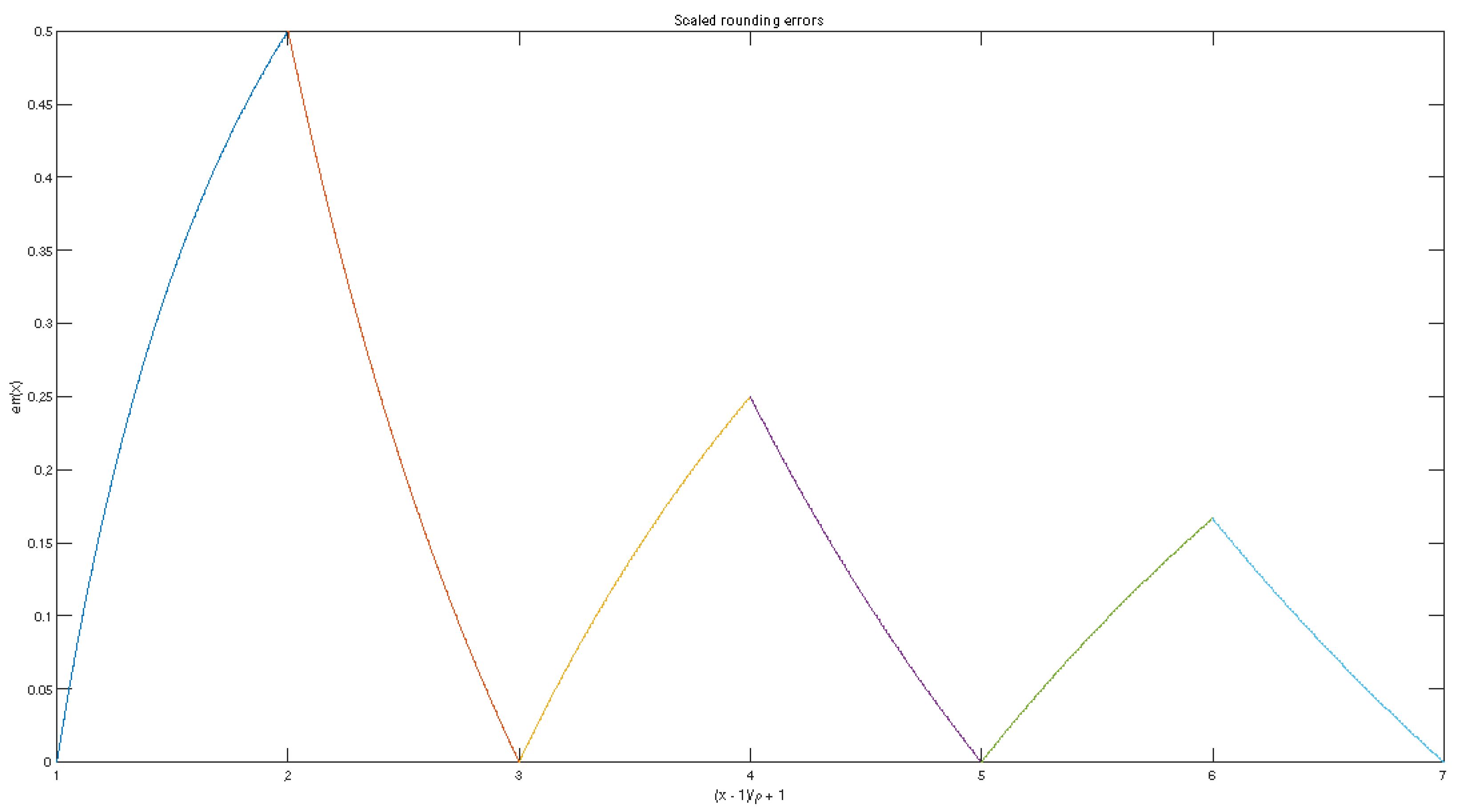
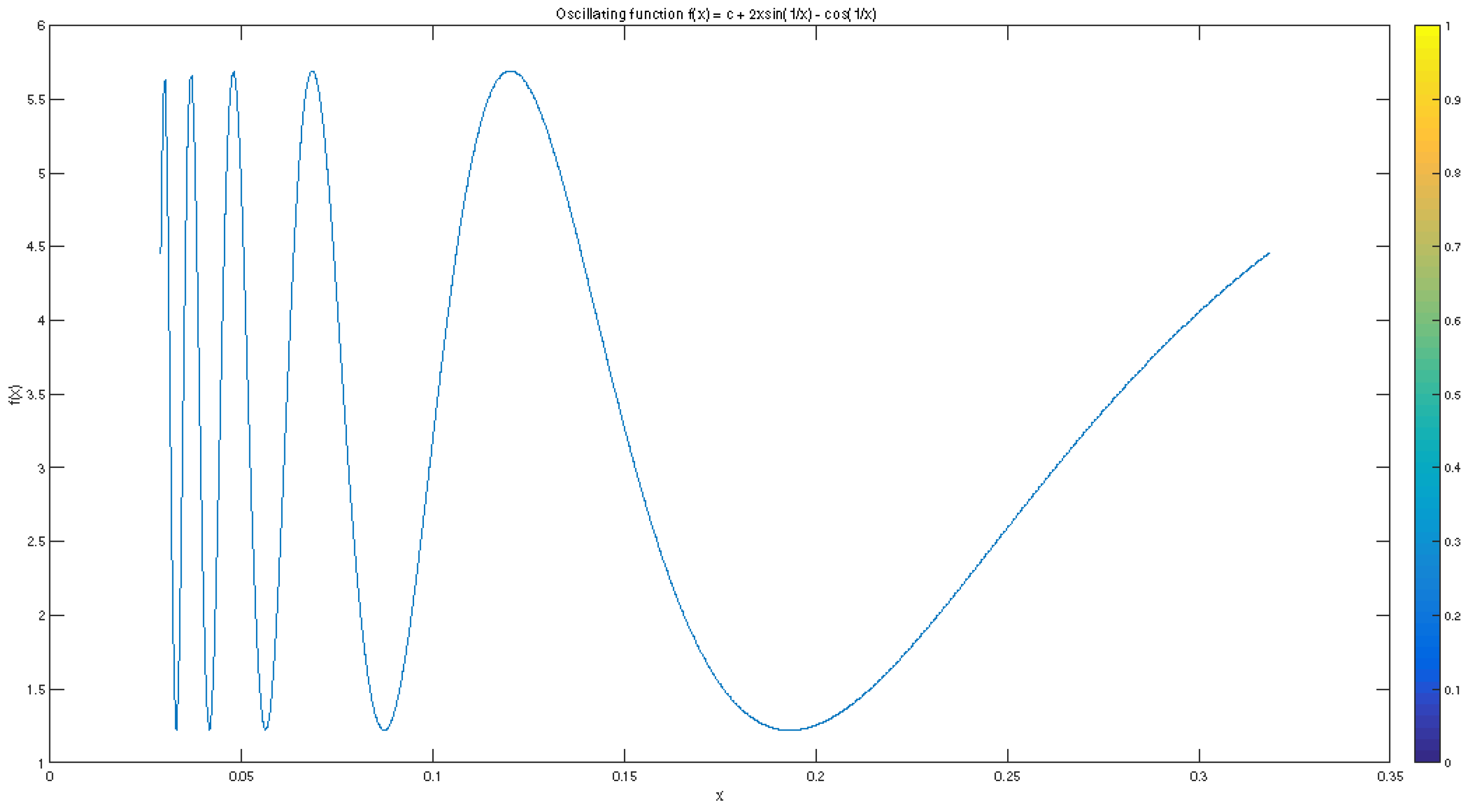
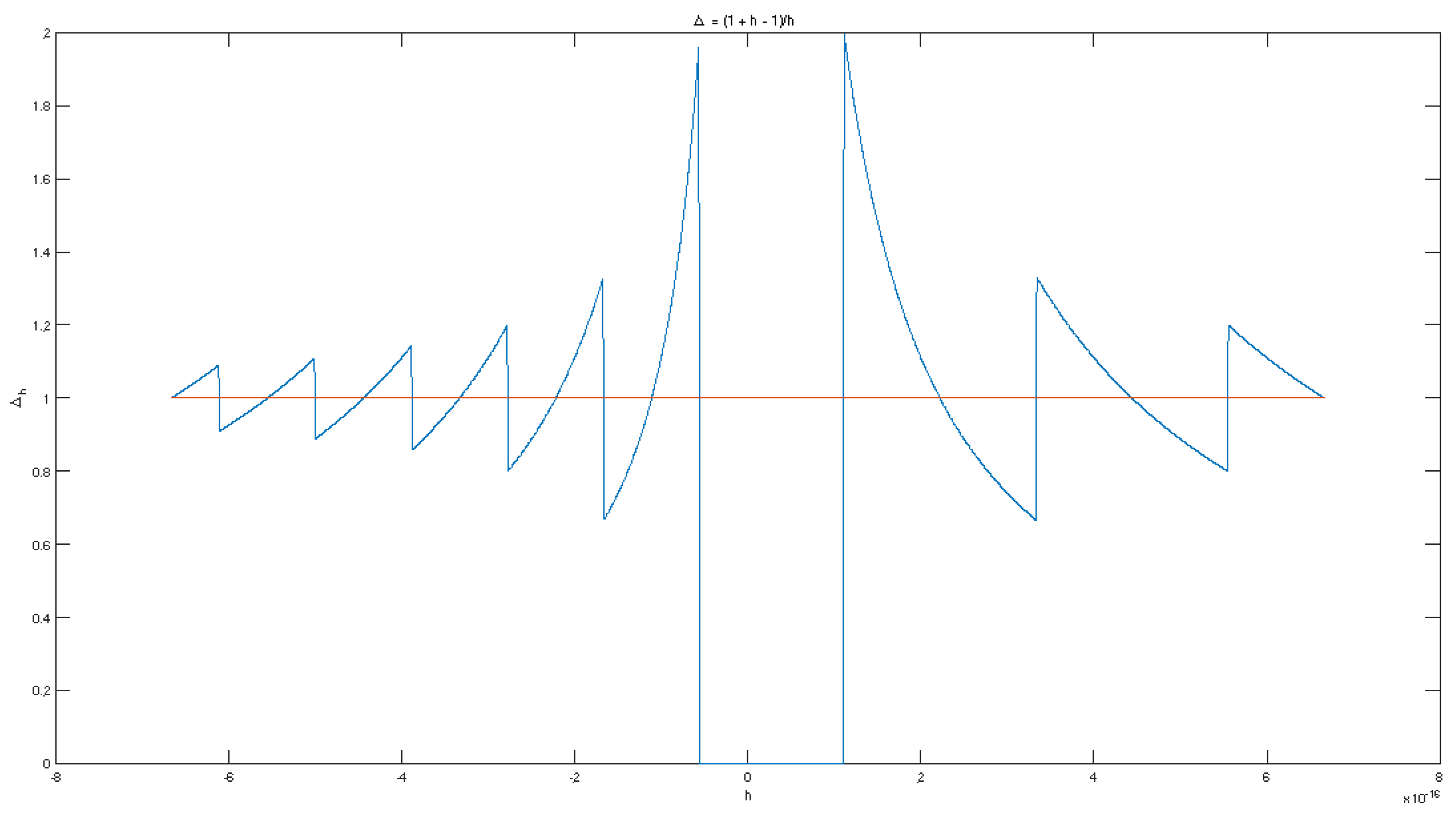
Disclaimer/Publisher’s Note: The statements, opinions and data contained in all publications are solely those of the individual author(s) and contributor(s) and not of MDPI and/or the editor(s). MDPI and/or the editor(s) disclaim responsibility for any injury to people or property resulting from any ideas, methods, instructions or products referred to in the content. |
© 2025 by the authors. Licensee MDPI, Basel, Switzerland. This article is an open access article distributed under the terms and conditions of the Creative Commons Attribution (CC BY) license (https://creativecommons.org/licenses/by/4.0/).