Bayesian Nonparametric Inference in Elliptic PDEs: Convergence Rates and Implementation ^†

Abstract

Parameter identification problems in partial differential equations (PDEs) consist in determining one or more functional coefficient in a PDE. In this article, the Bayesian nonparametric approach to such problems is considered. Focusing on the representative example of inferring the diffusivity function in an elliptic PDE from noisy observations of the PDE solution, the performance of Bayesian procedures based on Gaussian process priors is investigated. Building on recent developments in the literature, we derive novel asymptotic theoretical guarantees that establish posterior consistency and convergence rates for methodologically attractive Gaussian series priors based on the Dirichlet–Laplacian eigenbasis. An implementation of the associated posterior-based inference is provided and illustrated via a numerical simulation study, where excellent agreement with the theory is obtained.

1. Introduction

Partial differential equations (PDEs) are primary mathematical tools to model the behaviour of complex real-world phenomena, with ubiquitous applications across engineering and the sciences. The formulation of a PDE typically involves a number of functional parameters, which are often unknown in applications and not directly accessible to measurements. Employing a PDE model in practice therefore necessitates that the parameters in the equation be determined beforehand from the available data, giving rise to an inverse problem of parameter identification. Such problems have been extensively studied in applied mathematics [1,2,3] and, more recently, in statistics [4,5,6]. See the monographs [7,8,9] and the references therein for an extended overview on this research area.

In the present paper, we shall focus on the following representative example. Consider a physical quantity undergoing diffusion in an inhomogeneous multidimensional convex medium $\mathcal{O}\subset {\mathbb{R}}^d,d\in \mathbb{N}$, with smooth boundary $\partial \mathcal{O}$. At equilibrium, the density $u\left(x\right)$ of the diffusing substance at any location $x\in \mathcal{O}$ is governed by the second-order elliptic PDE

$$\left\{\begin{array}{cc}\nabla ·(f\nabla u)=s,\hfill & \mathrm{on}\mathcal{O}\hfill \\ u=b,\hfill & \mathrm{on}\partial \mathcal{O},\hfill \end{array}\right.$$

(1)

where $s:\mathcal{O}\to \mathbb{R}$ describes the spatial distribution of local sources or sinks, $g:\partial \mathcal{O}\to \mathbb{R}$ prescribes the density values at the boundary, and the diffusivity function $f:\mathcal{O}\to (0,\infty )$ models spatially varying conductivity throughout the inhomogeneous domain. Under mild regularity conditions on the PDE coefficients, standard elliptic theory implies the existence of a unique twice continuously differentiable classical solution $G\left(f\right)\equiv u_f\in C^2\left(\mathcal{O}\right)$ to (1) (e.g., [10], Chapter 6). Assuming that s and b are known, we are then interested in the problem of estimating f from n noisy point evaluations of $G\left(f\right)$ over a grid of (possibly random) design points $X_1,\dots ,X_n$ in $\mathcal{O}$,

$$Y_i=G\left(f\right)\left(X_i\right)+\sigma W_i,i=1,\dots ,n,$$

(2)

where $W_1,\dots ,W_n$ are statistical measurement errors, and $\sigma >0$ is the noise level. In view of the central limit theorem, the Gaussian assumption $W_1,\dots ,W_n\stackrel{iid}{\sim }N(0,1)$ can often be realistically maintained. The inverse problem of recovering the diffusivity in the elliptic PDE (1) from observations of its solution is an important building block in oil reservoir modelling [11], where u is the (accessible to measurements) fluid pressure, and f is the (not directly observable) permeability field, which can exhibit drastic spatial variations due to changes in the reservoir composition. This problem has been studied in a large number of articles in applied mathematics, e.g., [12,13,14], and statistics, e.g., [5,15,16]. An illustration on a bi-dimensional domain is given in Figure 1.

While the PDE (1) is linear, the parameter-to-solution map $f\mapsto G\left(f\right)$ is not, which poses several methodological and theoretical challenges. In particular, least squares functionals involving $G\left(f\right)$ are generally non-convex so that commonly used optimisation-based methods (such as Tikhonov regularisation, maximum likelihood or maximum-a posteriori estimation) cannot reliably be implemented by standard convex optimisation techniques. In this context, the Bayesian approach to inverse problems, popularised by influential work by Stuart [17], offers an attractive alternative. In the Bayesian framework, the unknown parameter f is regarded as a random variable (with values in a function space) and assigned a prior probability distribution $\Pi (·)$ that models the available information about f before collecting the observations. The prior is then combined, through Bayes’ formula, with the data ${\left\{(Y_i,X_i)\right\}}_{i=1}^n$ to form the posterior distribution $\Pi (·|{\left\{(Y_i,X_i)\right\}}_{i=1}^n)$, which represents the updated belief about f and is used to draw the inferences. As the posterior formally involves only evaluations of the prior and the likelihood (cf. Equation (7) below), the approximate computation of ${\Pi }_n(·|{\left\{(Y_i,X_i)\right\}}_{i=1}^n)$ and its associated posterior mean estimator ${\overline{f}}_n:=E^{\Pi }\left[f\right|{\left\{(Y_i,X_i)\right\}}_{i=1}^n]$ via sampling methods is feasible as long as the forward map G can be numerically evaluated. For  the elliptic PDE (1), this can be performed using efficient PDE solvers based on finite element methods, sidestepping altogether the need for a (possibly non-existent) inversion formula for G, as well as the use of optimisation approaches. In particular, for the class of Gaussian process priors, efficient ad hoc Markov chain Monte Carlo (MCMC) algorithms, suited to the present infinite-dimensional setting, have been developed, e.g., [16]. A further decisive advantage of the Bayesian methodology is that, alongside point estimates, it also automatically delivers uncertainty quantification for the recovery via the spread of the posterior, used in applications to provide interval-type estimators and to construct hypothesis tests.

The success and popularity in applications has led to recent interest in the literature for the derivation of theoretical performance guarantees for nonparametric Bayesian procedures in PDE models [18,19,20,21,22,23]. This is motivated by the fact that the performance of Bayesian methods depends on a suitable choice of the prior, which in infinite-dimensional statistical models primarily serves as a regularisation tool, and whose specification is a delicate task in its own right (cf. Section 1.2 in [24]). Thus, the question arises as to whether Bayesian procedures may provide valid and prior-independent inference, at least in the presence of informative data. The established paradigm under which such investigation is carried out is the frequentist analysis of Bayesian procedures, assuming that the observations are generated by a fixed ground truth $f_0$ and studying the concentration of the posterior towards $f_0$ in the large sample size limit. We refer the reader to [24] for an introduction to this research area.

The present paper is concerned with the performance of Bayesian nonparametric methods based on Gaussian priors in the elliptic inverse problem (2). In Section 2, we provide a general result that establishes posterior consistency and convergence rates of the conditional mean estimator for a general class of Gaussian priors (Theorem 1). We then apply our general theorem to obtain statistical recovery rates for truncated Gaussian series priors defined on the eigenbasis of the Dirichlet–Laplacian (Example 1), which is a commonly used basis of practical interest offering a convenient and generally applicable framework for implementation; cf. Section 3.1. This shows that the resulting procedures provide statistically valid estimation of the diffusivity f, with explicit estimation error bounds that decay algebraically in the number n of observations. Our results extend upon the recent investigation of Giordano and Nickl [20], who considered Gaussian priors associated to popular covariance kernels (such as the Matérn or squared-exponential ones), as well as truncated Gaussian wavelet series expansions but did not explore the methodologically attractive procedures based on the Dirichlet–Laplacian eigenbasis constructed herein.

Furthermore, in Section 3, we complement the theoretical results with a discussion on implementation, devising two different discretisation strategies. The first is tailored to applications where a specific set of basis functions is of interest. In particular, in Section 3.1, we employ the Dirichlet–Laplacian eigenbasis, discretising the parameter space by high-dimensional truncated series expansions in accordance with our theoretical results. In the second approach, described in Section 3.2, we discretise the parameter space via piece-wise linear functions defined on the elements of a deterministic triangular mesh, which is naturally suited to implementing Gaussian priors specified via a covariance kernel. Here, the popular Matérn kernel is employed for illustration. A numerical simulation study is provided to investigate the performance of the inferential procedures under the two discretisation strategies. In our numerical experiments, both approaches yielded satisfactory results, comparable in terms of reconstruction quality and running time. The posterior mean estimate (relative to a Matérn process prior), computed via a Metropolis–Hastings-type MCMC algorithm, is shown in Figure 2 for increasing sample sizes, to be compared to the true diffusion coefficient pictured in Figure 1 (left). The reproducible MATLAB code used for the study is available at https://github.com/MattGiord/Bayesian-Elliptic-PDEs/tree/main (accessed on 19 March 2025).

2. Materials and Methods

2.1. Likelihood, Prior and Posterior

Throughout, $\mathcal{O}\subset {\mathbb{R}}^d$, $d\in \mathbb{N}$, is a given nonempty, open, convex and bounded set with smooth boundary $\partial \mathcal{O}$. For the observation model (2), with $G\left(f\right)$ as the solution to the PDE (1), and for fixed constants $\alpha >1+d/2$ and $f_{min}>0$, we take the parameter space

$$\begin{array}{cc}\hfill & {\mathcal{F}}_{\alpha ,f_{min}}:=\left\{f\in H^{\alpha }\left(\mathcal{O}\right):\underset{x\in \mathcal{O}}{inf}f\left(x\right)\ge f_{min}, f_{|\partial \mathcal{O}}\equiv 1, {\displaystyle \frac{{\partial }^{j}f}{\partial {\nu }^j}}\equiv 0 for 1\le j\le \alpha -1\right\},\hfill \end{array}$$

(3)

with $H^{\alpha }\left(\mathcal{O}\right)$ as the usual Sobolev space of regularity $\alpha$ and $\nu \left(x\right),x\in \partial \mathcal{O}$, the unit normal vector. Assuming that the source term s in (1) is fixed and smooth, and taking (without loss of generality) homogeneous Dirichlet boundary conditions $b\equiv 0$, the Schauder theory for elliptic PDEs (e.g., Theorem 6.14 in [10]) implies that for each $f\in {\mathcal{F}}_{\alpha ,f_{min}}$, there exists a unique classical solution $G\left(f\right)\in C\left(\overline{\mathcal{O}}\right)\cap C^{1+\alpha }\left(\mathcal{O}\right)$ to the elliptic PDE (1). We then assume data ${\left\{(Y_i,X_i)\right\}}_{i=1}^n$ arising as in Equation (2) for some unknown $f\in {\mathcal{F}}_{\alpha ,f_{min}}$, with independent and identically distributed (i.i.d.) random design variables $X_1,\dots ,X_n$ following the uniform distribution on $\mathcal{O}$. Throughout, we regard the noise level $\sigma >0$ in (2) as fixed and known; in practice, it may often be replaced by an estimate (cf. Section 4). In view of the i.i.d. standard normal assumption on the noise variables $W_1,\dots ,W_n$ in (2), the random vectors ${\left\{(Y_i,X_i)\right\}}_{i=1}^n\sim P_f^{\left(n\right)}$ have joint probability density function in product form,

$$p_f^{\left(n\right)}\left({\left\{(x_i,y_i)\right\}}_{i=1}^n\right)={\displaystyle \frac{1}{{\left(2\pi {\sigma }^2\right)}^{n/2}}}{e}^{-{\sum }_{i=1}^n{[y_i-G\left(f\right)\left(x_i\right)]}^2/\left(2{\sigma }^2\right)},y_i\in \mathbb{R},x_i\in \mathcal{O}.$$

Accordingly, the log-likelihood is seen to be equal to, up to an additive constant, the negative least-square functional

$$l_n\left(f\right):=-{\displaystyle \frac{1}{2{\sigma }^2}}\sum _{i=1}^n{[Y_i-G\left(f\right)\left(X_i\right)]}^2,f\in {\mathcal{F}}_{\alpha ,f_{min}}.$$

(4)

In a recent paper by Giordano and Nickl [20], posterior consistency and convergence rates for the conditional mean estimator have been established for nonparametric Bayesian procedures based on Gaussian process priors. To incorporate the shape constraints in the parameter space ${\mathcal{F}}_{\alpha ,f_{min}}$, ref. [20] employed the parametrisation

$$f=\Phi \circ F,$$

(5)

where $F\in H_0^{\alpha }\left(\mathcal{O}\right)$ (the completion of $C_c^{\infty }\left(\mathcal{O}\right)$ with respect to ${\parallel ·\parallel }_{H^{\alpha }}$) and $\Phi :\mathbb{R}\to [f_{min},\infty )$ is a regular link function, that is a smooth, strictly increasing and bijective function with bounded derivatives and such that $\Phi \left(0\right)=1$. An instance of regular link function is provided in Example 24 of [20]. In practice, the exponential link $\Phi (·)=exp(·)$ is often used. In the following, we occasionally switch between the notation f and F, implicitly making use of the relation (5).

Under the parametrisation (5), placing a prior probability distribution $\Pi (·)$ on F induces a (push-forward) prior on f, which, in slight abuse of the notation, we still denote by $\Pi (·)$. Following [20], we consider scaled Gaussian priors, constructed starting from a base (possibly n-dependent) centred Gaussian Borel probability measure ${\Pi }_{W_n}$, which we assume to be supported on a measurable linear subspace of the Hölder space $C^{\beta }\left(\mathcal{O}\right)$, for some $\beta \ge 1$, and to have reproducing kernel Hilbert space (RKHS) ${\mathcal{H}}_{W_n}$ continuously embedded into $H_0^{\alpha }\left(\mathcal{O}\right)$. See Chapter 2 in [25] for the background and terminology on Gaussian processes and measures. Given ${\Pi }_{W_n}$, we then construct the scaled prior ${\Pi }_n(·)$ as the law of the random function

$$V\left(x\right):={\displaystyle \frac{W\left(x\right)}{n^{d/(4\alpha +4+2d)}}},x\in \mathcal{O},W\sim {\Pi }_{W_n}(·).$$

(6)

By linearity, ${\Pi }_n(·)$ also defines a centred Gaussian Borel probability measure with the same support as ${\Pi }_{W_n}$; the scaling enforces the additional regularisation used in the theoretical analysis to deal with the nonlinearity of the inverse problem.

Given prior ${\Pi }_n(·)$ as above, by Bayes’ formula (p. 7, [24]), the posterior distribution ${\Pi }_n(·|{\left\{(Y_i,X_i)\right\}}_{i=1}^n)$ of $F|{\left\{(Y_i,X_i)\right\}}_{i=1}^n$ arising from data in model (2) equals

$${\Pi }_n\left(B\right|{\left\{(Y_i,X_i)\right\}}_{i=1}^n)={\displaystyle \frac{{\int }_B{e}^{l_n(\Phi \circ F)}d{\Pi }_n\left(F\right)}{{\int }_{C\left(\mathcal{O}\right)}{e}^{l_n(\Phi \circ F^{\prime })}d{\Pi }_n\left(F^{\prime }\right)}},B\subseteq C\left(\mathcal{O}\right)measurable,$$

(7)

with $l_n(·)$ as the log-likelihood in (4).

2.2. Convergence Rates

We study the asymptotic concentration of the posterior distribution ${\Pi }_n(·|\left\{\right(Y_i,$$X_i{\left)\right\}}_{i=1}^n)$ in (7) around the ground truth diffusivity function $f_0=\Phi \circ F_0$, assuming that the data ${\left\{(Y_i,X_i)\right\}}_{i=1}^n\sim P_{f_0}^{\left(n\right)}$ have been generated according to the observation model (2) with $f=f_0$. The following theorem extends the main result of [20], allowing to include in the analysis general sieve-type Gaussian priors, cf. Example 1. The proof follows through similarly to Section 3.2 in [20]; it is included for completeness and the convenience of the reader in Appendix B.

Theorem 1.

For fixed positive integers $\alpha ,\beta \in \mathbb{N}$ such that $\alpha >\beta +d/2$, consider the scaled prior ${\Pi }_n$ in (6), where ${\Pi }_{W_n}$ is a centred Gaussian Borel probability measure supported on a measurable linear subspace of $C^{\beta }\left(\mathcal{O}\right)$, with RKHS ${\mathcal{H}}_{W_n}\subseteq H_0^{\alpha }\left(\mathcal{O}\right)$ satisfying, for some constant $c>0$ (independent of n),

$${\parallel F\parallel }_{H^{\alpha }}\le c{\parallel F\parallel }_{{\mathcal{H}}_{W_n}},\forall F\in {\mathcal{H}}_{W_n}.$$

Further assume that

$$\underset{n\in \mathbb{N}}{sup}{E}^{{\Pi }_{W_n}}{\parallel F\parallel }_{C^1}<\infty .$$

For fixed $F_0\in H_0^{\alpha }\left(\mathcal{O}\right)$, suppose that there exists a sequence $F_{0,n}\in {\mathcal{H}}_{W_n}$ such that, as $n\to \infty$,

$$\parallel F_0-F_{0,n}{\parallel }_{{\left(H^1\right)}^{\ast }}=O(n^{-{\displaystyle \frac{\alpha +1}{2\alpha +2+d}}});max\{\parallel F_{0,n}{\parallel }_{C^1},\parallel F_{0,n}{\parallel }_{{\mathcal{H}}_{W_n}}\}=O\left(1\right).$$

(8)

Then, there exists $L>0$ that is large enough such that, as $n\to \infty$,

$${\Pi }_n\left(f:\parallel G\left(f\right)-G\left(f_0\right){\parallel }_{L^2}>L{n}^{-{\displaystyle \frac{\alpha +1}{2\alpha +2+d}}}|{\left\{(Y_i,X_i)\right\}}_{i=1}^n\right)\to 0,$$

(9)

in $P_{f_0}^{(\infty )}$-probability as $n\to \infty$. If in addition $\beta \ge 2$ and ${inf}_{x\in \mathcal{O}}s\left(x\right)$$>0$, then there exists $L>0$ that is large enough and a constant $\lambda >0$ such that

$${\Pi }_n(f:\parallel f-f_0{\parallel }_{L^2} >L{n}^{-\lambda }\left|{\left\{(Y_i,X_i)\right\}}_{i=1}^n\right)\to 0,$$

(10)

in $P_{f_0}^{(\infty )}$-probability as $n\to \infty$, and moreover, the estimator ${\overline{f}}_n=\Phi \circ {\overline{F}}_n$, with ${\overline{F}}_n=E^{{\Pi }_n}\left[F\right|{\left\{(Y_i,X_i)\right\}}_{i=1}^n]$, satisfies as $n\to \infty$,

$$P_{f_0}^{\left(n\right)}\left(\parallel {\overline{f}}_n-f_0{\parallel }_{L^2} >n^{-\lambda }\right)\to 0.$$

(11)

The first statement (Equation (9)) of Theorem 1 establishes posterior consistency in prediction risk: The induced posterior on the PDE solution $G\left(f\right),f\sim {\Pi }_n(·|\left\{\right(Y_i,$$X_i{\left)\right\}}_{i=1}^n)$, concentrates around the true PDE solution $G\left(f_0\right)$ in $L^2$-distance at rate $n^{-(\alpha +1)/(2\alpha +2+d)}$. Since such a rate is known to be minimax optimal [26] (Theorem 10), procedures satisfying the assumption of Theorem 1 are seen to optimally solve the PDE-constrained regression problem of recovering $G\left(f_0\right)$ from data ${\left\{(Y_i,X_i)\right\}}_{i=1}^n$.

The second statement shows that the posterior contracts around $f_0$ also in the standard $L^2$-risk, thereby solving the inverse problem of estimating the diffusivity. It follows combining (9) with the regularisation properties implied by the rescaling in the prior construction (6) and a suitable stability estimate for $G^{-1}$. The latter was proved in [26] (Lemma 24), and requires the slightly stronger assumption on $\beta$ and the strict positivity of the source s. The exponent $\lambda >0$ is explicitly computed in the proof of Theorem 1 and equals $\lambda =(\alpha +1)(\beta -1)/(2\alpha +2+d)(\beta +1)$. Note that $\lambda <(\alpha +1)/(2\alpha +2+d)$. While minimax optimal rates for estimating the diffusivity f in model (2) are currently unknown, inspection of the proof shows that when $f_0\in C^{\infty }\left(\mathcal{O}\right)$, then the prior can be tuned so to attain a rate as closed as desired to the parametric rate $n^{-1/2}$.

The last statement of Theorem 1 entails that the estimator ${\overline{f}}_n$ converges towards $f_0$ in $L^2$-risk at the same rate $n^{-\lambda }$ attained by the whole posterior distribution. It is indeed a corollary of (10), following from uniform integrability arguments for Gaussian measures and the Lipschitzianity of the composition with the link function $\Phi$.

2.3. Examples of Gaussian Priors

We now provide two concrete instances of Gaussian priors to which Theorem 1 applies. For both examples, an implementation of the associated posterior-based inference is provided in Section 3 below. We maintain the assumption that $f_0=\Phi \circ F_0$ for some $F_0\in H^{\alpha }\left(\mathcal{O}\right)$ supported inside a given compact subset $K\subset \mathcal{O}$. This corresponds to the common assumption that $f_0$ is known near the boundary $\partial \mathcal{O}$ (specifically $f_0\equiv 1$ on $\mathcal{O}\setminus K$).

We first consider high-dimensional Gaussian sieve priors obtained via truncating Karhunen–Loève-type random series expansions, a frequently used approach in computation, e.g., [27]. In particular, via Theorem 1, we study procedures based on the Dirichlet–Laplacian eigenbasis. Such constructions corresponds to commonly used Gaussian process priors with covariance kernel given by an inverse power of the Laplacian, e.g., [17] (Section 2.4). The eigenbasis can be numerically computed via efficient finite element methods for elliptic eigenvalue problems, offering a broadly applicable framework for implementation on general domains $\mathcal{O}$. Details on computation and a numerical simulation study are provided in Section 3.1.

Example 1

(Dirichlet–Laplacian eigenbasis). Let $\{e_j,j\ge 0\}\subset H_0^1\left(\mathcal{O}\right)\cap C^{\infty }\left(\overline{\mathcal{O}}\right)$ be the orthonormal basis of $L^2\left(\mathcal{O}\right)$ formed by the eigenfunctions of the (negative) Dirichlet–Laplacian:

$$\left\{\begin{array}{cc}-\Delta e_j-{\lambda }_j{e}_j=0,\hfill & \mathrm{on}\mathcal{O}\hfill \\ e_j=0,\hfill & \mathrm{on}\partial \mathcal{O},\hfill \end{array}\right.j\ge 0,$$

(12)

with associated eigenvalues $0<{\lambda }_0<{\lambda }_1\le {\lambda }_2\le \dots ,$ satisfying ${\lambda }_j\to \infty$ as $j\to \infty$ according to Weyl’s asymptotics: ${\lambda }_j=O\left(j^{2/d}\right)$ as $j\to \infty$, cf. Figure 3 and Figure 4. See Example 6.3 and Section 7.4 in [28] for details. Define the Hilbert scale

$${\mathbb{H}}^s:=\left\{w\in L^2{\left(\mathcal{O}\right):\parallel w\parallel }_{{\mathbb{H}}^s}^2:=\sum _{j=0}^{\infty }{\lambda }_j^s{\left|{\langle w,e_j\rangle }_2\right|}^2<\infty \right\},s\ge 0.$$

We then have ${\mathbb{H}}^0=L^2\left(\mathcal{O}\right)$ (with equality of norms), ${\mathbb{H}}^1=H_0^1\left(\mathcal{O}\right)$ (with equivalence of norms), ${\mathbb{H}}^2=H_0^1\left(\mathcal{O}\right)\cap H^2\left(\mathcal{O}\right)$, and the continuous embedding ${\mathbb{H}}^s\subset H^s\left(\mathcal{O}\right)$ for all $s\ge 0$ (holding generally with strict inclusion), cf. p. 472f. in [29]. In fact, it holds that ${\parallel w\parallel }_{{\mathbb{H}}^s}\simeq {\parallel w\parallel }_{H^s}$ for all $w\in {\mathbb{H}}^s$ and $s\ge 0$ (proved initially for $s=2$, then extended by induction to all larger integers, and finally by interpolation to all positive reals), and if $F\in H^s\left(\mathcal{O}\right)$ is compactly supported within $\mathcal{O}$, then $F\in {\mathbb{H}}^s$. Finally, defining ${\mathbb{H}}^{-1}:={\left({\mathbb{H}}^1\right)}^{\ast }={\left(H_0^1\left(\mathcal{O}\right)\right)}^{\ast }$, we have the equivalence (cf. Equation (A15) in [29])

$$\begin{array}{c}\hfill {\parallel w\parallel }_{{\left(H_0^1\right)}^{\ast }}^2\simeq {\parallel w\parallel }_{{\mathbb{H}}^{-1}}^2:=\sum _{j=0}^{\infty }{\lambda }_j^{-1}{\left|{\langle w,e_j\rangle }_2\right|}^2.\end{array}$$

(13)

Now for fixed $J\in \mathbb{N}$, the Gaussian random sum

$${\overline{W}}_J:=\sum _{j\le J}{\lambda }_j^{-\alpha /2}{W}_j{e}_j,W_j\stackrel{iid}{\sim }N(0,1),$$

defines a centred Gaussian Borel probability measure supported on (and with RKHS equal to) the finite-dimensional space ${\mathcal{H}}_{{\overline{W}}_J}:=\mathrm{span}\{e_j,j\le J\}$, with RKHS norm

$$\parallel \overline{w}{\parallel }_{{\mathcal{H}}_{{\overline{W}}_J}}^2=\sum _{j\le J}{\lambda }_j^{\alpha }{w}_j^2=\parallel \overline{w}{\parallel }_{{\mathbb{H}}^{\alpha }}^2\simeq {\parallel \overline{w}\parallel }_{H^{\alpha }}^2,\forall w\in {\overline{W}}_J.$$

Fix any smooth cut-off function $\chi \in C_c^{\infty }\left(\mathcal{O}\right)$ such that $\chi =1$ on K, and consider the random function

$$W_n:=\chi W_{J_n}=\sum _{j\le J_n}{\lambda }_j^{-\alpha /2}{W}_j\chi e_j,W_j\stackrel{iid}{\sim }N(0,1),$$

(14)

where $J_n\in \mathbb{N}$ is such that $J_n\simeq n^{d/(2\alpha +2+d)}$. By the linearity and boundedness of multiplication by χ, the law ${\Pi }_{W_n}$ of $W_n$ defines, according to Exercise 2.6.5 in [25], a centred Gaussian prior supported on (and with RKHS equal to)

$${\mathcal{H}}_{W_n}=\mathrm{span}\{\chi e_j,j\le J_n\}\subset C_c^{\infty }\left(\mathcal{O}\right)\subset \bigcap _{s=0}^{\infty }{H}_0^s\left(\mathcal{O}\right)\cap \bigcap _{s=0}^{\infty }{\mathbb{H}}^s,$$

with RKHS norm satisfying, with a multiplicative constant independent of n,

$$\parallel \chi \overline{w}{\parallel }_{{\mathcal{H}}_{W_n}} \le \parallel \overline{w}{\parallel }_{{\mathcal{H}}_{{\overline{W}}_{J_n}}}\simeq {\parallel \overline{w}\parallel }_{H^{\alpha }},\forall \overline{w}\in {\mathcal{H}}_{{\overline{W}}_{J_n}}.$$

Arguing as in Example 25 in [20], one further shows that for some constant $c>0$ (independent of n),

$${\parallel w\parallel }_{H^{\alpha }}\le c{\parallel w\parallel }_{{\mathcal{H}}_{W_n}},\forall w\in {\mathcal{H}}_{W_n}.$$

Finally, by a Sobolev embedding and the above inequality,

$$\begin{array}{cc}\hfill E^{{\Pi }_{W_n}}{\parallel F\parallel }_{C^1}^2 & \lesssim E^{{\Pi }_{W_n}}{\parallel F\parallel }_{H^{\alpha }}^2\le c{E}^{{\Pi }_{W_n}}{\parallel F\parallel }_{{\mathcal{H}}_{W_n}}^2\le E\left[\sum _{j\le J_n}{\lambda }_j^{-\alpha }{W}_j^2\right],\hfill \end{array}$$

which is uniformly bounded in n recalling that $W_i\stackrel{iid}{\sim }N(0,1)$ and the fact that by Weyl’s asymptotics ${\lambda }_j^{-\alpha }=O\left(j^{-2\alpha /d}\right)$ with $\alpha >1+d/2$. This shows that the sequence of base priors ${\Pi }_{W_n}$ satisfies the first two assumptions of Theorem 1. For ground truths $F_0\in H^{\alpha }\left(\mathcal{O}\right)$ compactly supported inside K, we have $F_0\in {\mathbb{H}}^{\alpha }$. Construct the finite-dimensional approximations

$$F_{0,n}=\sum _{j\le J_n}{\langle F_0,e_j\rangle }_2\chi e_j\in {\mathcal{H}}_{W_n},n\in \mathbb{N}.$$

(15)

Then for all $n\in \mathbb{N}$,

$$\begin{array}{cc}\hfill \parallel F_{0,n}{\parallel }_{{\mathcal{H}}_{W_n}} & \le {∥\sum _{j\le J_n}{\langle F_0,e_j\rangle }_2{e}_j∥}_{{\mathcal{H}}_{{\overline{W}}_{J_n}}}={∥\sum _{j\le J_n}{\langle F_0,e_j\rangle }_2{e}_j∥}_{{\mathbb{H}}^{\alpha }} \le \parallel F_0{\parallel }_{{\mathbb{H}}^{\alpha }}\simeq {\parallel F_0\parallel }_{H^{\alpha }}<\infty .\hfill \end{array}$$

By a Sobolev embedding, we similarly have $\parallel F_{0,n}{\parallel }_{C^1}\le {\parallel F_0\parallel }_{H^{\alpha }}<\infty$ for all $n\in \mathbb{N}$. Furthermore, since both $F_0$ and $F_{0,n}$ have compact support within $\mathcal{O}$,

$$\begin{array}{cc}\hfill \parallel F_0-F_{0,n}{\parallel }_{{\left(H^1\right)}^{\ast }}& =\underset{H\in H^1\left(\mathcal{O}\right)}{sup}{\int }_{\mathcal{O}}(F_0\left(x\right)-F_{0,n}\left(x\right))H\left(x\right)dx\hfill \\ \hfill & =\underset{H\in H_0^1\left(\mathcal{O}\right)}{sup}{\int }_{\mathcal{O}}(F_0\left(x\right)-F_{0,n}\left(x\right))H\left(x\right)dx={\parallel F_0-F_{0,n}\parallel }_{{\left(H_0^1\right)}^{\ast }},\hfill \end{array}$$

and recalling (13), Weyl’s asymptotics, and the choice of $J_n$,

$$\begin{array}{cc}\hfill \parallel F_0-F_{0,n}{\parallel }_{{\left(H^1\right)}^{\ast }}^2 & =\sum _{j>J_n}{\lambda }_j^{-(1+\alpha )}{\lambda }_j^{\alpha }{\left|{\langle F_0,e_j\rangle }_2\right|}^2\hfill \\ \hfill & \le {\lambda }_{J_n}^{-(1+\alpha )}{\parallel F_0\parallel }_{{\mathbb{H}}^{\alpha }}^2\lesssim {\left(J_n\right)}^{-2(1+\alpha )/d}\simeq n^{-2(\alpha +1)/(2\alpha +2+d)}.\hfill \end{array}$$

We conclude that Theorem 1 applies with the sequence of base Gaussian sieve priors in (14), choosing the approximations $F_{0,n}$ according to (15).

The second main example, already considered in [20], concerns stationary Gaussian processes specified via a translation invariant covariance kernel. For concreteness, we focus on the popular Matérn kernel. Implementation of the resulting procedures is illustrated in Section 3.2.

Example 2

(Matérn covariance kernel). Consider a Matérn process $W=\left\{W\right(x),x\in \mathcal{O}\}$ on $\mathcal{O}$ with regularity $\alpha -d/2$, that is a centred stationary Gaussian process with covariance kernel

$$C(x,y)={\displaystyle \frac{2^{1-\alpha }}{\Gamma \left(\alpha \right)}}{\left({\displaystyle \frac{|x-y|\sqrt{2\alpha }}{\ell }}\right)}^{\alpha }{B}_{\alpha }\left({\displaystyle \frac{|x-y|\sqrt{2\alpha }}{\ell }}\right),x,y\in \mathcal{O},\ell >0,$$

(16)

where Γ denotes the gamma function and $B_{\alpha }$ is the modified Bessel function of the second kind. Fix any smooth cut-off function $\chi \in C_c^{\infty }\left(\mathcal{O}\right)$ such that $\chi =1$ on K. It can then be shown (cf. Example 25 in [20]) that the law ${\Pi }_W$ of $\chi W$ defines a centred Gaussian Borel probability measure supported on the separable linear subspace $C^{{\beta }^{\prime }}\left(\mathcal{O}\right)$ of $C^{\beta }\left(\mathcal{O}\right)$ for any $\beta <{\beta }^{\prime }<\alpha -d/2$. Furthermore, its RKHS is given by ${\mathcal{H}}_W=\{\chi F,F\in H^{\alpha }\left(\mathcal{O}\right)\}\subset H_0^{\alpha }\left(\mathcal{O}\right)$, with the RKHS norm satisfying

$${\parallel \chi F\parallel }_{H^{\alpha }}\lesssim {\parallel \chi F\parallel }_{{\mathcal{H}}_W},\forall F\in H^{\alpha }\left(\mathcal{O}\right).$$

For ground truths $F_0\in H^{\alpha }\left(\mathcal{O}\right)$ compactly supported inside K, we have $\chi F=F$, so that $F\in {\mathcal{H}}_W$. We conclude that Theorem 1 applies for a base Matérn process prior ${\Pi }_{W_n}:={\Pi }_W$, choosing the trivial approximating sequence $F_{0,n}:=F_0$ for all $n\in \mathbb{N}$.

3. Results

We investigate the performance of the procedures based on the Gaussian priors considered in Examples 1 and 2 in a numerical simulation study. For illustration, we fix the working domain $\mathcal{O}$ to the area contained inside the rotated ellipse, with $\theta =\pi /6$,

$$\partial \mathcal{O}=\left\{\right(cos\left(t\right)cos\left(\theta \right)-0.75sin\left(t\right)sin\left(\theta \right),0.75sin\left(t\right)cos\left(\theta \right)+cos\left(t\right)sin\left(\theta \right)),t\in [0,2\pi \left)\right\},$$

and take the ground truth conductivity

$$\begin{array}{cc}\hfill f_0(x,y) & =\sum _{k,m\in \{-1,1\}}{e}^{-{(5x+1.75k)}^2-{(5y+1.75m)}^2},(x,y)\in \mathcal{O},\hfill \end{array}$$

(17)

cf. Figure 1 (left). We then generate observations ${\left\{(Y_i,X_i)\right\}}_{i=1}^n$ according to (2). The true PDE solution $G\left(f_0\right)$ is numerically computed via finite element methods, using the MATLAB PDE Toolbox. For the experiments, the source function is set to $s(x,y)=exp(-{(5x-2.5)}^2-{\left(5y\right)}^2)+exp(-{\left(7.5x\right)}^2-{\left(2.5y\right)}^2)+exp(-{(5x+2.5)}^2-{\left(5y\right)}^2),(x,y)\in \mathcal{O}$, and the noise standard deviation to $\sigma =0.0025$ (with corresponding signal-to-noise ratio $\parallel G\left(f_0\right){\parallel }_{L^2}/\sigma =68.50$). Further experiments, with differently shaped ground truths, are presented in Appendix A.

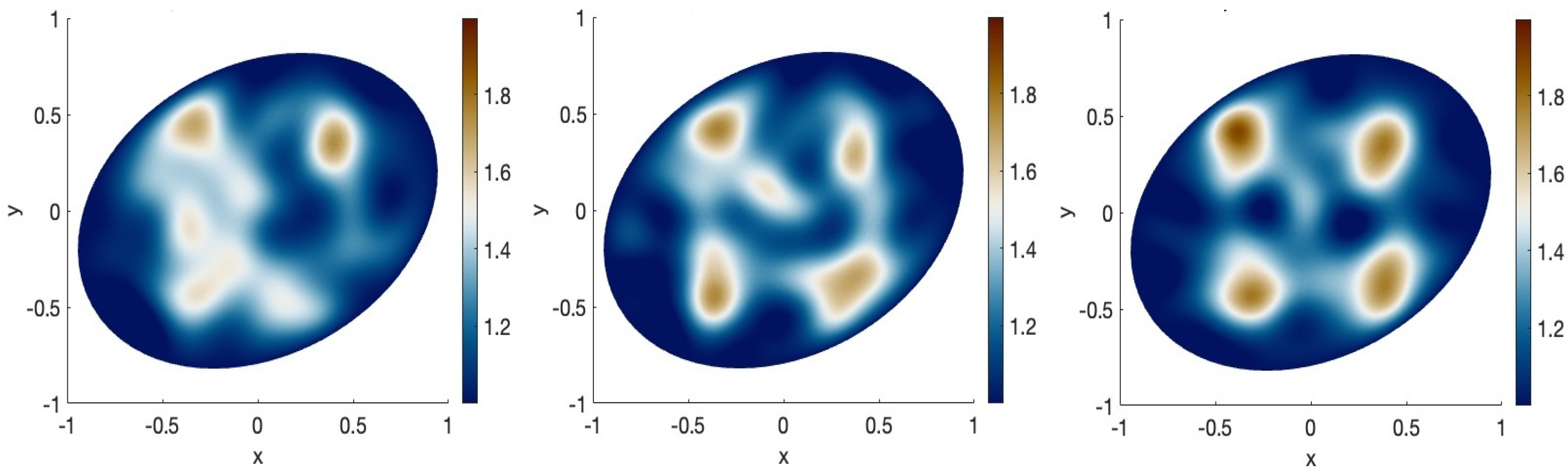
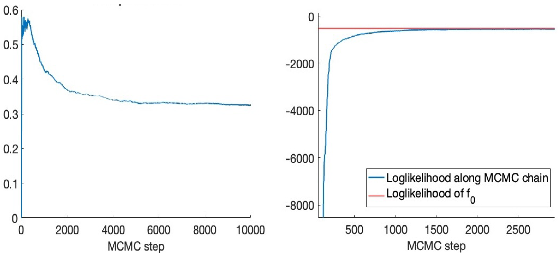
3.1. Results with Truncated Gaussian Series Priors

To implement the truncated Gaussian series priors from Example 1, we numerically compute the first $J_n\simeq n^{d/(2\alpha +2+d)}$ Dirichlet–Laplacian eigenpairs via finite element methods; see Figure 3 and Figure 4. Identifying the functional parameter F in (5) with the vector of coefficients $\mathbf{F}:=[F_1,\dots ,F_{J_n}]$, where $F_j:={\langle F,e_j\rangle }_2$, the prior then corresponds to

$$\mathbf{F}\sim N(0,{\Lambda }_n),{\Lambda }_n:=n^{-d/(2\alpha +2+d)}\mathrm{diag}({\lambda }_1^{-\alpha },\dots ,{\lambda }_{J_n}^{-\alpha })\in {\mathbb{R}}^{J_n,J_n}.$$

(18)

While the employed prior is Gaussian, the nonlinearity of the forward map $f\mapsto G\left(f\right)$ implies that the log-likelihood $l_n\left(f\right)$ in (4) depends nonlinearly on f. The resulting posterior distribution is therefore generally non-Gaussian and not available in closed form. We then resort to MCMC sampling via the pCN algorithm [16], which is a specific instance of the random-walk Metropolis–Hastings method for Gaussian priors that is known to be robust to the discretisation dimension. In the present setting, we employ the pCN algorithm to generate an ${\mathbb{R}}^{J_n}$-valued Markov chain ${\left({\mathbf{F}}_h\right)}_{h\ge 1}$ with invariant measure equal to the posterior distribution, starting from an initialisation point ${\mathbf{F}}_0$ and then, for $h=0,1,2,\dots$, repeating the following steps:

• Draw a prior sample $\xi \sim N(0,{\Lambda }_n)$, where ${\Lambda }_n$ is as in (18), and for $\delta >0$ define the proposal $p:=\sqrt{1-2\delta }{\mathbf{F}}_h+\sqrt{2\delta }\xi$;
• Set

  $${\mathbf{F}}_{h+1}:=\left\{\begin{array}{cc}p,\hfill & \mathrm{with} \mathrm{probability}1\wedge e^{l(\Phi \circ p)-l(\Phi \circ {\mathbf{F}}_h)},\hfill \\ {\mathbf{F}}_h,\hfill & \mathrm{otherwise},\hfill \end{array}\right.$$

  where l is the log-likelihood function in (4).

For each iteration, step 2 requires the evaluation of the log-likelihood $l_n(\Phi \circ p)$, which in turn entails the numerical evaluation of the PDE solution $G(\Phi \circ p)$ at the design points $X_1,\dots ,X_n$, cf. (4), which we perform via finite element methods. The prior samples $\xi \sim N(0,{\Lambda }_n)$ required in step 1 are straightforward to draw since ${\Lambda }_n$ is diagonal.

The algorithm is terminated after H steps, returning approximate samples $\{{\mathbf{F}}_0,h=0,$$\dots ,$$H\}$ from the posterior distribution, where a first batch of iterates is typically discarded as the burn-in. Under a set of assumptions on the forward map that is compatible with the present setting, Hairer, Stuart, and Vollmer [30] derived dimension-free spectral gaps which imply rapid convergence of the pCN marginal laws towards the invariant measure. As a consequence, the posterior mean ${\overline{F}}_n$ can reliably be numerically computed by the MCMC average

$$\overline{\mathbf{F}}:={\displaystyle \frac{1}{H+1}}\sum _{h=0}^H{\mathbf{F}}_h,$$

(19)

with non-asymptotic bounds for the numerical approximation error. Posterior credible sets can likewise be reliably computed by considering the empirical quantiles of the pCN samples.

Figure 2 shows the posterior mean estimates ${\overline{f}}_n=\Phi \circ {\overline{F}}_n$ of the conductivity function f obtained for increasing sample sizes $n=100,250,1000$. The corresponding $L^2$ estimation errors (and the associated relative errors) are reported in

Table 1. $L^2$-estimation errors and relative errors for the posterior mean estimates with increasing sample sizes.

n	100	250	500	1000
$\parallel {\overline{f}}_n-f_0{\parallel }_{L^2}$; series prior	0.2981	0.2232	0.2144	0.1581
$\parallel {\overline{f}}_n-f_0{\parallel }_2/{\parallel f_0\parallel }_{L^2}$; series prior	17.67%	12.23%	12.71%	9.36%
$\parallel {\overline{f}}_n-f_0{\parallel }_{L^2}$; Matérn prior	0.3289	0.2677	0.2033	0.1647
$\parallel {\overline{f}}_n-f_0{\parallel }_2/{\parallel f_0\parallel }_{L^2}$; Matérn prior	18.98%	15.86%	12.05%	9.76%

(first and second row), displaying a progressive decay as expected from the theory developed in Section 2. Across the experiments, the prior regularity parameter $\alpha$ in Equation (18) is set to $\alpha =3=2+d/2$. The pCN algorithm is iterated H = 25,000 times, and the first 5000 samples are discarded as the burn-in. The step size is set to $\delta =0.0025,0.001,0.0005,0.00025$, tuned depending on the sample size to obtain a stabilisation of the acceptance rate around 30% after the burn-in; see Figure 5 (left). A pCN cold-start ${\mathbf{F}}_0=0$ is employed. Figure 5 (right) shows, for the experiment with $n=1000$, the log-likelihood $l_n(\Phi \circ {\vartheta }_h)$ along the first 3000 pCN iterates (part of the burn-in phase), seen to rapidly increase towards, and then stabilise around, the log-likelihood $l_n\left(f_0\right)$ attained by the true diffusivity $f_0$. The computation time per experiment is around 50 min on a 2020 M1 MacBook Pro 13 running MATLAB 2024b.

3.2. Results with the Matérn Process Prior

For Gaussian process priors specified via a covariance kernel, such as the Matérn process considered in Example 2, we discretise the parameter space by assuming that F in (5) is given by the finite sum

$$F=\sum _{m=1}^M{F}_m{\psi }_m,F_m\in \mathbb{R},M\in \mathbb{N},$$

(20)

where $\{{\psi }_1,\dots ,{\psi }_M\}$ are piecewise linear functions on a deterministic triangular mesh with nodes $\{z_1,\dots ,z_M\}\subset \mathcal{O}$, uniquely characterised by the relation ${\psi }_m\left(z_{m^{\prime }}\right)=1_{\{m=m^{\prime }\}}$. Accordingly, F in (20) satisfies $F\left(z_m\right)=F_m$, and for any $x\in \mathcal{O}$, the value $F\left(x\right)$ is obtained by linear interpolation over the pairs $\{(z_m,F_m),m=1,\dots ,M\}$. Given the Matérn kernel C in (16), and identifying F with the vector of values $\mathbf{F}:=[F_1,\dots ,F_M]$, the prior then corresponds to

$$\mathbf{F}\sim N(0,\mathbf{C}),\mathbf{C}={\left[C_{m{m}^{\prime }}\right]}_{m,m^{\prime }=1}^M\in {\mathbb{R}}^{M,M},C_{m{m}^{\prime }}=C(z_m,z_m^{\prime }).$$

Posterior inference based on the Matérn process prior may be implemented via the pCN algorithm described in Section 3.1 above. For each iteration, the construction of the pCN proposal p in step 1 entails sampling an independent multivariate Gaussian random variable $\xi \sim N(0,\mathbf{C})$. In step 2, the computation of the acceptance probability requires the evaluation of the proposal log-likelihood $l_n(\Phi \circ p)$, which can be performed via numerical PDE methods as described above.

For the ground truth $f_0$ specified in Equation (17), Table 1 (third and fourth row) displays the $L^2$-estimation errors (and the relative errors) associated to the posterior mean estimates ${\overline{f}}_n=\Phi \circ {\overline{F}}_n$ for increasing sample sizes $n=100,250,500,1000$. Across the experiments, the parameter space is discretised using a uniform triangular mesh with $M=2000$ nodes. The hyperparameters for the Matérn covariance kernel in (16) are set to $\alpha =3$ and $\ell =0.25$. Similarly to the results in Section 3.1, the runs of pCN are stopped after H = 25,000 iterations, with a tuning of the step size (respectively, $\delta =0.0025,0.001,0.0005,0.00025$) to achieve a stabilisation of the acceptance rate at around $30\%$ after the burn-in (corresponding to the first 5000 iterates). A non-informative initialisation point ${\mathbf{F}}_0=0$ is chosen for each run. The computation times ranges between 50 and 57 min, in line with those obtained for the truncated Gaussian series prior in Section 3.1.

4. Discussion

In this article, we have considered the nonparametric Bayesian approach to inference in elliptic PDEs, focusing on the standard benchmark problem of estimating the diffusivity function from noisy observation of the PDE solution. We have provided a general asymptotic concentration result, Theorem 1, for the posterior distribution and the posterior mean estimator, and showed that it applies to two classes of Gaussian priors of interest, namely truncated Gaussian series priors defined on the Dirichlet–Laplacian eigenbasis (cf. Example 1) and Matérn process priors (cf. Example 2). For both prior models, we have devised strategies for implementing the posterior-based inference, employing efficient and reliable MCMC algorithms. The performance of the considered methods has been investigated in a numerical simulation study, where excellent reconstruction results and a general agreement with the theory have been obtained. Overall, the main advantages of the approach lie in its modelling flexibility, and the robustness of the associated computational methods, as well as the availability of theoretical guarantees on the recovery performance.

Let us conclude overviewing some related research questions. Firstly, we remark that that the noise standard deviation $\sigma$ in (2) is assumed to be known throughout the paper. In the realistic scenario where $\sigma$ is also unknown, the methodology developed here can readily be adapted by replacing it (in an empirical Bayes spirit) with a preliminary (non-likelihood-based) estimate. Several strategies have been proposed in the literature for variance estimation in nonparametric regression models, ranging from residual-based estimators using kernel smoothing [31] and splines [32], to difference-based estimators [33]. Alternatively, a joint Bayesian model for f and $\sigma$ in (2) could be considered by endowing $\sigma$ with a prior distribution (for example, an independent conjugate inverse gamma prior). This leads to the interesting question concerning the extension of the theoretical results presented in Section 2 to the setting with unknown variance; see [34] for related results in a direct regression model.

Secondly, we mention the important issue of specifying the hyperparameter values for the considered prior distributions, namely, the regularity parameter $\alpha$ for the truncated Gaussian series prior from Example 1, and the smoothness and length-scale in the Matérn covariance kernel (16). There a vast literature investigating the methodological and theoretical aspects of empirical and hierarchical Bayesian strategies to fully data-driven hyperparameters selection; see [20,35,36,37,38], where many more references can be found. Investigating the implications and performance of these methods in the context of the elliptic PDE model and the Gaussian prior distributions considered in the present article is an interesting direction for future research.

References

1. Engl, H.W.; Hanke, M.; Neubauer, A. Regularization of Inverse Problems; Mathematics and Its Applications; Kluwer Academic Publishers Group: Dordrecht, The Netherlands, 1996; Volume 375, p. viii+321. [Google Scholar]
2. Kaltenbacher, B.; Neubauer, A.; Scherzer, O. Iterative Regularization Methods for Nonlinear Ill-Posed Problems; Radon Series on Computational and Applied Mathematics; Walter de Gruyter GmbH & Co. KG: Berlin, Germany, 2008; Volume 6, p. viii+194. [Google Scholar] [CrossRef]
3. Isakov, V. Inverse Problems for Partial Differential Equations, 3rd ed.; Applied Mathematical Sciences; Springer: Cham, Switzerland, 2017; Volume 127, p. xv+406. [Google Scholar] [CrossRef]
4. Kaipio, J.; Somersalo, E. Statistical and Computational Inverse Problems; Number 160 in Applied Mathematical Sciences; Springer: New York, NY, USA, 2004. [Google Scholar]
5. Bissantz, N.; Hohage, T.; Munk, A. Consistency and rates of convergence of nonlinear Tikhonov regularization with random noise. Inverse Probl. 2004, 20, 1773–1789. [Google Scholar] [CrossRef]
6. Hohage, T.; Pricop, M. Nonlinear Tikhonov regularization in Hilbert scales for inverse boundary value problems with random noise. Inverse Probl. Imaging 2008, 2, 271–290. [Google Scholar] [CrossRef]
7. Benning, M.; Burger, M. Modern regularization methods for inverse problems. Acta Numer. 2018, 27, 1–111. [Google Scholar] [CrossRef]
8. Arridge, S.; Maass, P.; Öktem, O.; Schönlieb, C.B. Solving inverse problems using data-driven models. Acta Numer. 2019, 28, 1–174. [Google Scholar] [CrossRef]
9. Nickl, R. Bayesian Non-Linear Statistical Inverse Problems; Zurich Lectures in Advanced Mathematics; EMS Press: Berlin, Germany, 2023; p. xi+15. [Google Scholar] [CrossRef]
10. Evans, L.C. Partial Differential Equations, 2nd ed.; Graduate Studies in Mathematics; American Mathematical Society: Providence, RI, USA, 2010; Volume 19, p. xxii+749. [Google Scholar] [CrossRef]
11. Yeh, W.W.G. Review of Parameter Identification Procedures in Groundwater Hydrology: The Inverse Problem. Water Resour. Res. 1986, 22, 95–108. [Google Scholar] [CrossRef]
12. Richter, G.R. An inverse problem for the steady state diffusion equation. SIAM J. Appl. Math. 1981, 41, 210–221. [Google Scholar] [CrossRef]
13. Knowles, I. Parameter identification for elliptic problems. J. Comput. Appl. Math. 2001, 131, 175–194. [Google Scholar] [CrossRef]
14. Bonito, A.; Cohen, A.; DeVore, R.; Petrova, G.; Welper, G. Diffusion coefficients estimation for elliptic partial differential equations. SIAM J. Math. Anal. 2017, 49, 1570–1592. [Google Scholar] [CrossRef]
15. Dashti, M.; Stuart, A.M. Uncertainty quantification and weak approximation of an elliptic inverse problem. SIAM J. Numer. Anal. 2011, 49, 2524–2542. [Google Scholar] [CrossRef]
16. Cotter, S.; Roberts, G.; Stuart, A.; White, D. MCMC Methods for Functions: Modifying Old Algorithms to Make Them Faster. Stat. Sci. 2013, 28, 424–446. [Google Scholar] [CrossRef]
17. Stuart, A.M. Inverse problems: A Bayesian perspective. Acta Numer. 2010, 19, 451–559. [Google Scholar] [CrossRef]
18. Vollmer, S.J. Posterior consistency for Bayesian inverse problems through stability and regression results. Inverse Probl. 2013, 29, 125011. [Google Scholar] [CrossRef]
19. Abraham, K.; Nickl, R. On statistical Calderón problems. Math. Stat. Learn. 2019, 2, 165–216. [Google Scholar] [CrossRef]
20. Giordano, M.; Nickl, R. Consistency of Bayesian inference with Gaussian process priors in an elliptic inverse problem. Inverse Probl. 2020, 36, 85001–85036. [Google Scholar] [CrossRef]
21. Monard, F.; Nickl, R.; Paternain, G.P. Consistent inversion of noisy non-Abelian X-ray transforms. Comm. Pure Appl. Math. 2021, 74, 1045–1099. [Google Scholar] [CrossRef]
22. Giordano, M. Asymptotic Theory for Bayesian Nonparametric Inference in Statistical Models Arising from Partial Differential Equations. Doctoral Thesis, University of Cambridge, Cambridge, UK, 2021. [Google Scholar] [CrossRef]
23. Agapiou, S.; Wang, S. Laplace priors and spatial inhomogeneity in Bayesian inverse problems. Bernoulli 2024, 30, 878–910. [Google Scholar] [CrossRef]
24. Ghosal, S.; van der Vaart, A.W. Fundamentals of Nonparametric Bayesian Inference; Cambridge University Press: New York, NY, USA, 2017. [Google Scholar]
25. Giné, E.; Nickl, R. Mathematical Foundations of Infinite-Dimensional Statistical Models; Cambridge University Press: New York, NY, USA, 2016; p. xiv+690. [Google Scholar] [CrossRef]
26. Nickl, R.; van de Geer, S.; Wang, S. Convergence rates for penalized least squares estimators in PDE constrained regression problems. SIAM/ASA J. Uncertain. Quantif. 2020, 8, 374–413. [Google Scholar] [CrossRef]
27. Dashti, M.; Stuart, A.M. The Bayesian approach to inverse problems. In Handbook of Uncertainty Quantification; Springer: Cham, Switzerland, 2017; pp. 311–428. [Google Scholar]
28. Haroske, D.D.; Triebel, H. Distributions, Sobolev Spaces, Elliptic Equations. EMS Press: Berlin, Germany, 2007. [Google Scholar]
29. Taylor, M.E. Partial Differential Equations I; Springer: New York, NY, USA, 2011. [Google Scholar]
30. Hairer, M.; Stuart, A.; Vollmer, S. Spectral Gaps for a Metropolis-Hastings Algorithm in Infinite Dimensions. Ann. Appl. Probab. 2014, 24, 2455–2490. [Google Scholar] [CrossRef]
31. Hall, P.; Marron, J. On variance estimation in nonparametric regression. Biometrika 1990, 77, 415–419. [Google Scholar] [CrossRef]
32. Wahba, G. Improper priors, spline smoothing and the problem of guarding against model errors in regression. J. R. Stat. Soc. Ser. B Stat. Methodol. 1978, 40, 364–372. [Google Scholar] [CrossRef]
33. Rice, J. Bandwidth choice for nonparametric regression. Ann. Statist. 1984, 12, 1215–1230. [Google Scholar] [CrossRef]
34. Kejzlar, V.; Son, M.; Bhattacharya, S.; Maiti, T. A fast and calibrated computer model emulator: An empirical Bayes approach. Stat. Comput. 2021, 31, 49. [Google Scholar] [CrossRef]
35. Knapik, B.; Szabò, B.; van der Vaart, A.W.; van Zanten, H. Bayes procedures for adaptive inference in inverse problems for the white noise model. Probab. Theory Relat. Fields 2015, 164, 771–813. [Google Scholar] [CrossRef]
36. Rousseau, J.; Szabo, B. Asymptotic behaviour of the empirical Bayes posteriors associated to maximum marginal likelihood estimator. Ann. Stat. 2017, 45, 833–865. [Google Scholar] [CrossRef] [PubMed]
37. Teckentrup, A.L. Convergence of Gaussian process regression with estimated hyper-parameters and applications in Bayesian inverse problems. SIAM/ASA J. Uncertain. Quantif. 2020, 8, 1310–1337. [Google Scholar] [CrossRef]
38. Agapiou, S.; Bardsley, J.M.; Papaspiliopoulos, O.; Stuart, A.M. Analysis of the Gibbs sampler for hierarchical inverse problems. SIAM/ASA J. Uncertain. Quantif. 2014, 2, 511–544. [Google Scholar] [CrossRef]
39. Giordano, M.; Ray, K. Nonparametric Bayesian inference for reversible multidimensional diffusions. Ann. Stat. 2022, 50, 2872–2898. [Google Scholar] [CrossRef]
40. Li, W.V.; Linde, W. Approximation, metric entropy and small ball estimates for Gaussian measures. Ann. Probab. 1999, 27, 1556–1578. [Google Scholar] [CrossRef]
Figure 1. (Left): An example of diffusivity function f with four circular regions of higher conductivity. (Right): n = 4500 noisy observations from the corresponding PDE solution G ( f ) .
Foundations 05 00014 g001
Figure 2. Left to right: posterior mean estimates f ¯ n of the diffusivity function f for increasing sample sizes n = 100 , 250 , 1000 .
Foundations 05 00014 g002
Figure 3. Left to right: The first, second, and fiftieth Dirichlet–Laplacian eigenfunctions e 0 , e 1 and e 49 , computed via finite element methods.
Foundations 05 00014 g003
Figure 4. Dirichlet–Laplacian eigenvalues λ j in the range [ 0 , 500 ] , computed via finite element methods.
Foundations 05 00014 g004
Figure 5. (Left): acceptance rate over the first 10,000 pCN samples. The rate stabilises around 30 % after the initial burn-in time (first 5000 iterates). (Right): in blue, the log-likelihood l n ( Φ ϑ h ) of the first 3000 iterates; in red, the log-likelihood l n ( f 0 ) of the true diffusion coefficient f 0 .
Foundations 05 00014 g005