Abstract
The often used analytical representation of the Maxwell–Boltzmann classical speed distribution function (F) for elastic, indivisible particles assumes an infinite limit for the speed. Consequently, volume and the number of particles (n) extend to infinity: Both infinities contradict assumptions underlying this non-relativistic formulation. Finite average kinetic energy and temperature (T) result from normalization of F removing n: However, total energy (i.e., heat of the collection) remains infinite because n is infinite. This problem persists in recent adaptations. To better address real (finite) systems, wherein T depends on heat, we generalize this one-parameter distribution (F, cast in energy) by proposing a two-parameter gamma distribution function (F*) in energy which reduces to F at large n. Its expectation value of kT (k = Boltzmann’s constant) replicates F, whereas the shape factor depends on n and affects the averages, as expected for finite systems. We validate F* via a first-principle, molecular dynamics numerical model of energy and momentum conserving collisions for 26, 182, and 728 particles in three-dimensional physical space. Dimensionless calculations provide generally applicable results; a total of 107 collisions suffice to represent an equilibrated collection. Our numerical results show that individual momentum conserving collisions in three-dimensions provide symmetrical speed distributions in all Cartesian directions. Thus, momentum and energy conserving collisions are the physical cause for equipartitioning of energy: Validity of this theorem for other systems depends on their specific motions. Our numerical results set upper limits on kinetic energy of individual particles; restrict the n particles to some finite volume; and lead to a formula in terms of n for conserving total energy when utilizing F* for convenience. Implications of our findings on matter under extreme conditions are briefly discussed.
1. Introduction
The Maxwell-Boltzmann speed distribution function (F) describes a collection of (n) indivisible, elastic particles at thermal equilibrium, with only one parameter, temperature (T), e.g., [1,2,3]. As detailed below, F in this classical, non-relativistic representation provides the probability density as a function of speed for the collection. Maxwell’s [4,5] model, as modified by Boltzmann [6,7], is important because it not only propelled development of classical statistical mechanics and thermal physics, but remains relevant to studies of negative entropy [8] and plasma physics [9]. Yet, discrepancies with experiments exist [10,11,12,13]. Why real, non-relativistic systems depart from the classical speed distribution F needs elucidating.
Maxwell’s collection of particles may be viewed as a gas composed of miniscule hard spheres each with mass (m), or as point masses that can collide. Translational motions are the sole form of energy and thus the total kinetic energy constitutes the heat of the collection per the kinetic theory of gas [1,2]. Commonly used presentations of the continuous speed (u) distribution pertain to u from 0 to ∞, and account for the scalar u not depending on angular variables:
where k is Boltzmann’s constant [1,2,14].
The speed of the ith particle is defined by its directional velocity (v) components, which give the particle’s kinetic energy (E):
The root mean speed <u2> is obtained by dividing by n and integrating to infinity:
where integrating over the dummy variable, q ≡ ½mu2/(kT), gives the gamma function: specifically, Γ(5/2) = ¾π½. Rearranging Equation (3) yields the average (kinetic) energy:
Equation (4) has only been validated by experiments describing limited circumstances. Namely, it is supported by the ideal gas law through considering Clausius’ Virial Theorem [15,16], and by heat capacity data on monatomic gases near ambient temperature, e.g., [17] (p. 587). Consequently, the following holds:
- General applicability of Maxwell–Boltzmann’s speed distribution to real systems has not been demonstrated.
Analytical forms that are bounded during integration are highly convenient. Although shortcomings associated with F(u)du extending to u = ∞ for non-relativistic systems are recognized, their importance has been dismissed based on low values of F at high u. However:
- Formulae for the averages (speed, energy, and temperature in Equations (3) and (4)) incorporate non-zero values of F(u) that exist at impossibly large u.
- Consequently, the total energy for the collection of particles (i.e., its heat) is affected by the number of particles occupying these high energy states at low values for F(u) as the infinite limit of u is approached.
- Overestimates of average energy result due to the length of the distribution’s tail to infinity, and because a continuous function assumes continuous values of speed.
Additional problems are associated with infinite speed in non-relativistic situations:
- The space occupied by the collection is unbounded over finite time, due to u → ∞, which conflicts with the assumption that the particles occupy some finite volume, as in real systems.
- The limits of infinite speed in an infinite volume requires an infinite number of particles, otherwise negligible collisions occur and approaching equilibrium is impossible: Both contradict the assumptions.
- The total energy:is also infinite, because integrals extending to u → ∞ not only require that E → ∞, but also that n → ∞. In detail, infinite Etot means that any finite amount of energy can be added to (or removed from) the system but the total energy remains the same (∞). Thus, creation (and destruction) of energy is permitted mathematically in the continuous representation of Maxwell’s distribution function. Energy conservation is violated.
- Heat in the Maxwellian gas is thus also described by the limit of infinity, since translation motions define its thermal energy. Yet, T is finite, which conflicts with a key principle of classical thermodynamics: namely, that heat and temperature are related, albeit distinct, entities. In a classical, non-relativistic system, a finite temperature would be accompanied by a finite amount of heat.
Violation of total energy conservation is obscured by n not entering into the averages of Equations (3) or (4). The absence of n gives the appearance of the averages being independent of n, which is untrue for any system of moving particles. In a finite n system, the applied heat (Etot) is divided among the particles, so a large n system must have a lower temperature than a small n systems under identical Etot. Conservation would be possible if n had been an explicit part of the averages.
The unrealistic infinities are hidden due to the limited role of n. This parameter serves only to constrain the numerical coefficients of F(u) via normalization:
where integrating over q yields Γ(3/2) = ½π½. Moreover, the statistically important probability distribution function (PDF) of speed is obtained by dividing F by n and normalizing the area under the curve to unity, thereby entirely removing particle number from the PDF. For further details, see e.g., [1,2,14].
1.1. Purpose of the Present Paper
Real, measurable systems are finite, no matter how large n might be. Based on the above, we suggest that discrepancies of the classical formulation with experiments [10,11,12,13] originate in the infinities, which in turn stem from the infinitesimal being an essential component of a continuous function.
Although incorporating relativity reduces the maximum particle speed from infinity to light-speed, this change does not remedy the other problems listed above. Specifically, n remains infinite, and so the total energy and system’s physical volume also remain infinite. Thus, energy is still not conserved. Also, temperature and heat would remain disconnected in a relativistic modification. Using relativistic corrections for finite particle numbers will still result in the possibility of individual particles exceeding system energy. Thus, the effect of finite particle number needs to be delineated before exploring the effect of limiting the maximum velocity. Revisiting Maxwell’s non-relativistic speed distribution, with a focus on finite n, is therefore warranted.
Examination of the above equations shows the following.
- Violation of energy conservation is tied to the average energy not depending on particle number (Equation (4)).
Hence, we explicitly incorporate n into our analytical exploration of non-relativistic, finite systems. To the best of our knowledge, generalizations of F that include n have not previously been published.
As is common in statistical analysis, we consider a continuous analytical function and thus implicitly assume that n is quite large. Infinities are present in virtually all analytical distribution functions. This approach is used because it provides equations that can be integrated and to closed-form solutions. The advancement sought in the present study is to find a distribution function for which n is not removed during normalization. Achieving this goal should yield a relationship between temperature and heat.
Because discrepancies should be most apparent when n is small, we furthermore use a numerical approach to calculate how velocities and kinetic energies are distributed among a collection with a modest number of particles, but after many (107) collisions. Three different n-values are explored.
Combining these independent, complementary analytical and numerical methods permits evaluating the accuracy of our proposal of an alternative PDF. Our approach should further understanding of thermal behavior of real collections which have a finite number of particles.
Additional reasons exist to explore the effect of finite n on the speed distribution:
- Statistics of small numbers is of long-standing interest (e.g., Poisson’s discrete distribution function [18]) and remains of widespread interest today [19].
- Regarding the behavior of matter, small n is relevant as T approaches absolute zero and kinetic motions dwindle, which limits the physical volume where collisions occur.
- Extremely high density likewise restricts particle motions to a small volume, but for the contrasting reason of frequent rebounds.
- Extremely low density is of interest due to possible effects on collision probabilities and attaining equilibrium. Effects of rarefication may pertain to the cosmological question regarding temperatures and mass in intergalactic media, which remains unresolved [20], and so means of detecting high-T media are still being sought [21].
1.2. Organization of the Paper
Motivation for this study is described above (Section 1.1). The analytical component of this paper (Section 2) begins by recognizing that Equation (1) is a one-parameter statistical formulation. The classical formula is then generalized by including n in a continuous PDF with two parameters. We show that the proposed function adheres to classical thermodynamic precepts. Section 3 clarifies assumptions underlying Maxwell’s approach, which we implemented (Section 4.1) in constructing our numerical, molecular dynamics model for elastic collisions of a finite number of particles. Numerical results (Section 4.2) validate our proposed two-parameter PDF. Section 4.2.3 describes how our numerical results depend on n and provides formulae. Section 4.2.4 provides details on the energy distribution function, focusing on the presence of an upper limit. Section 5 covers implications of our analytical and numerical results. This discussion section describes ways to incorporate conservation of energy into convenient, analytical formulations. Section 5 also revisits the importance of volume, and notes possible future work. Section 6 concludes with some implications of our findings.
2. Proposed Two-Parameter Energy PDF
Per Maxwell, redistribution of kinetic energy (E = ½mu2) achieves equilibrium. The condition is better described as steady-state, but this term was not used during the development of thermodynamics since Fourier’s heat transfer theory was not incorporated [22,23].
Formulae for kinetic energy distributions are derived from Equations (1) and (2) incorporating speed:
(e.g., [14]). Recasting uses dE, rather than d(E/kT), to account for experimental data being measured as a function of E, not of E/kT.
Maxwell’s formulation is a statistical representation of the energetics of a collection of indivisible particles [24]. Equation (7), being statistical in nature, has an expectation (or expected) value (Θ) of kT. The expected value for E need not equal the average energy [25]. Section 3.2 explains why Θ equals kT from a perspective not discussed previously, to the best of our knowledge.
2.1. Proposed New Distribution Function
Addressing the relationship between heat and temperature requires a more complicated statistical model than Equation (7). That the energy PDF (right hand side RHS of Equation (7)) only involves a single parameter, T, signals that the distribution is too simple and that something has been omitted. The missing factor is particle number, per the discussion of Section 1.
To incorporate heat (total energy), which is proportional to the key parameter n (Equation (5)), we base our proposed PDF on the two-parameter gamma family [26,27] (p. 230 ff), defined as follows:
where the expectation value Θ (also known as the scale factor) and the shape factor κ compose the two parameters of the two-parameter gamma function in x, which is a placeholder, and does not indicate position, see [26,27]. Erlang [28] appears to be the originator of the gamma distribution (considering integer values of κ): his work postdated the efforts of Maxwell and Boltzmann.
We considered other two-parameter functions and found that the two-parameter gamma function is the best representation of the energetics of a collection of indivisible particles. Equation (8) is the optimal choice because it reduces to Equation (7) at large n, as follows:
For an energy distribution function, x equals E. Comparing Equations (7) and (8) shows that the expectation value Θ in F* equals kT as in F. This comparison leads us to propose the following two-parameter kinetic energy distribution functions:
which have the following attributes [26]:
A shape factor of κ = 3/2 reproduces Equation (7), i.e., Maxwell’s energy distribution function, and thus represents very large n. Consistently, κ = 3/2 returns the classical result of <E> = 3kT/2, as in Equation (4).
2.2. Properties of Our Proposed Two-Parameter Distribution Function
Features of Equation (9) are as follows. Under constant applied heat (=Etotal), T increases as n decreases. This behavior is expected for a real system.
As a consequence, the mean increases with T while the variance (κΘ2 = κk2T2) increases more strongly. These two behaviors are dictated by Equation (10), as follows: Under constant T, <E> = Etotal/n increases as n decreases, as expected. Hence, κ increases as n decreases. For constant T, the variance increases as n decreases and at the same rate as the mean energy increases. Inverting the middle equation in the top row of Equation (10) provides the following:
2.3. Summary
Because κ depends on n, as described above, our proposal distinguishes heat (total energy) from temperature (an energy average) as required by classical thermodynamics. Thus, our proposal (Equations (9) and (10)) meets one of our goals (Section 1.1).
We also sought a function with a finite limit. Very few exist. The beta function [27,29] is one example, but a finite limit is obtained by defining the distribution function as equaling 0 for x > 1. As such, the beta distribution has three parameters, the cutoff of unity being the third. Our proposed function could likewise be truncated at some value of E. However, this stipulation amounts to either an arbitrary constraint or an additional parameter.
The problem with infinite total energy is inherent to an analytical approach using a continuous function. To make inroads into this long-standing problem in statistical physics, Section 4 presents numerical methods to investigate distributions for small, finite n.
3. Classical Theory
3.1. Assumptions Underlying Maxwell’s Speed Distribution Function
For our numerical model to rest on a similar set of approximations as those underlying Maxwell’s speed distribution function, we need to understand what approximations were made. We begin with Weaver’s [24] summary of Maxwell’s assumptions and then discuss their validity and relationship to the present work. From Weaver [24]:
- Collisions are elastic.
- The constituent particles interact by means of central repulsive forces.
- The distribution is statistical.
- Every direction of particle rebound subsequent to a binary collision is equally probable.
- If Assumptions 3 and 4 are both true, then (i) all three velocity components of any involved velocity have independent probability distributions and (ii) every displacement direction is as likely as every other.
To Weaver’s [24] list, we add the following:
- 6.
- It is implied in Maxwell’s approach that the n particles occupy some isolated volume (V) in physical space (Figure 1a). This is evident in the renormalization condition (Equation (6)) and in assuming the gas is at thermodynamic equilibrium [1].
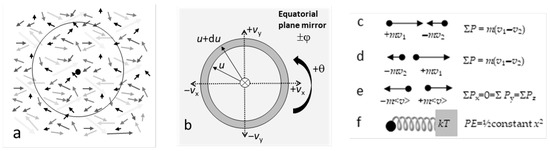 Figure 1. Schematics of motions collapsed onto a plane: (a) Particles in a gas. Arrows suggest random directions of motions with various speeds. Dot = center enclosed by an imaginary volume (circle), which is sufficiently large to represent equilibrium conditions; (b) Velocity space coordinates, showing the mirror (light grey) and 2-fold rotational axis (circle with ×) of a non-translating system; (c) Conditions preceding a head-on one-dimensional collision of two particles; (d) Conditions after a head-on momentum- and energy-conserving collision; (e) Momentum balance during equilibrium. After many conservative collisions, a non-translating system must have momentum magnitudes that are equal, on average, in the three orthogonal directions; (f) Harmonic oscillator (ball and spring) in equilibrium with a heat reservoir (grey block), which is one-dimensional with both KE and potential energy (PE).
 - 7.
- The system does not translate or rotate.
- 8.
- Collisions involve two particles, but not multiple particles.
The elastic approximation (Assumption 1) requires that energy and momentum are conserved during each and every collision, which has several implications (Section 3.2). Assumption 2 is valid, but its implications have gone unrecognized (Section 3.3). Because Maxwell’s approach is statistical (Assumption 3), he did not consider motions of either individual particles or of pairs of colliding particles. His statistical approach requires very large n and renders the travel direction of an individual particle irrelevant under momentum conservation (discussed below). Irrelevance of direction is consistent with kinetic energy being the quantity that is redistributed (Equation (7)).
Assumption 4, that all directions of travel are equally probable after a collision, while valid statistically, does not apply to individual particles colliding elastically. Rather, momentum and energy conservation define the trajectories of the two particles afterward given that particles at that time were viewed as indivisible, nearly point masses which cannot rotate. If the particles were rotating, collisions might have an angular dependence, but this would not be random. Moreover, if the velocities depended on angular variables, then the averages of Equations (3) and (4) would not be obtained. Thus, by assuming elasticity, Maxwell’s construction does not follow Assumption 4 of Weaver, listed above. Instead, the construction actually makes a different assumption, so we replace Weaver’s Assumption 4 with the followind, denoted Assumption 4*:
4.* Velocity space of the collection is radially symmetric (Figure 1b).
Furthermore, radial symmetry of velocity space leads to total momentum conservation. Section 3.2 provides details.
Assumption 5 from Weaver [24] is actually a conclusion, and does not describe individual behavior, but may hold statistically, if n is very large. Combining Assumptions 1, 3, 4* and 7 leads to a different conclusion than Assumption 5, see Section 3.2. Assumption 6 (finite volume) is equivalent to assuming that the collection of particles is a bound state (further discussion and implications are given in Section 3.4).
Lastly, Assumption 8 stems from the kinetic theory of gas. KTG presumes that collisions are brief compared to the time between collisions [1]. Thus, over any given time interval, the particles mainly translate without interacting. For this reason, collision of several particles at once is unexpected, and was not considered by Maxwell, or in the present paper.
3.2. Why Total Momentum Is Conserved
Considering only the radial component of velocity space (Figure 1b) mathematically reduces the problem of a collection of particles in three-dimensional physical space to one-dimensional velocity space. Because longitude (θ) and latitude (φ) are otherwise required to describe individual particle motions, using a spherically symmetric velocity space assumes balanced distribution of + and − velocity vectors for each direction at any instant of time over the collection.
The overall directional balance describes a non-translating, non-rotating system. Balancing velocity vectors originates in momentum conservation during each collision (Figure 1c–e). A non-translating system further requires conservation of total linear momentum in all three directions. Hence:
- The statistical distributions of the velocities in each direction are equal, which originates in elastic individual collisions in a non-translating, non-rotating system.
- The distributions are interrelated but are certainly not independent as described in Assumption 5 of Section 3.1.
Partitioning is discussed further below (Section 3.4).
3.3. Potential Energy and Implications for the Expectation Value
Although kinetic energy has been the focus, potential energy (PE) necessarily exists for two reasons:
- Central forces (Assumption 2 of Section 3.1) are conservative and always have an associated potential. This localized potential applies to colliding pairs of particles.
- The system is a bound state (Assumption 6 of Section 3.1) which requires PE for the collection as a whole, since without some binding energy the particles would disperse. Dispersion precludes attaining thermal equilibrium, which is assumed in order to describe the gas of colliding particles in terms of temperature.
The existence of the global or collective potential has no other effect than to create the bound state of the collection. Thus, detailed discussion of the collective potential is not needed. Implications of the bound state are covered in Section 3.4.
In contrast, the localized potential directly pertains to the expectation value (kT), which regulates the exponential partitioning of the translational kinetic energy (KE = E = ½mu2). However, the localized potential was not discussed by Maxwell because he treated collisions as a geometric redirection, rather than as a deceleration and acceleration by some specific force. We thus discuss the effects of potential energy from the perspective of reversals, which are events required by momentum conservation. In this regard, the harmonic oscillator is used as a guide (or reference point), because harmonic oscillations include not only reversals but, moreover, involve a conservative potential. Two additional reasons for comparing collisions to harmonic oscillations exist:
- (1)
- As in the case of the harmonic oscillator (Figure 1f), the colliding particles have two degrees of freedom due to the various back-and-forth motions which define the volume that a single particle influences. This depiction is closely allied with Clausius’ concept of a sphere of action surrounding any given particle [30] and underlies Maxwell’s Assumption 2 (Section 3.1), see [24].
- (2)
- In a statistical sense, reversals constitute oscillations. Moreover, oscillatory behavior is mandated for two limiting cases for the gas of particles. One case is a one-dimensional system, where the particles cannot travel through each other. The second limiting case is n = 2 (Figure 1c,d), for which a bound state (Assumption 6 of Section 3.1) requires that the two particles oscillate about their center of mass.
An expectation value of kT results for elastic collisions because this represents the average total energy (PE + KE) of an isolated harmonic oscillator and also of a collection of oscillators [1] (p. 252). If only KE existed, the expectation value would be 3/2 kT to represent the three directions in space, see e.g., Ref [1] (p. 250ff) for examples.
Similar to colliding pairs of particles in the gas, individual oscillators in a collection are randomly oriented. As in the gas, the energy of the average oscillating particle is related to that of the collection (i.e., the reservoir of Figure 1f). The average energy need not equal the expectation value [25,26,27]. For the case at hand, the expectation value reflects the role of potential energy in directional changes during collisions (Assumption 2 in Section 3.1), which has not heretofore been recognized.
3.4. Effect of the Bound State on Energy Partitioning
Because Maxwell’s distribution describes a volumetric bound state (Assumption 6, Section 3.1), the Virial Theorem [15] must hold, where the average kinetic energy is proportional to the average potential energy. The proportionality constant depends on the form for the central force: For a force depending directly on distance, the averages of KE and PE are equal, see [16].
From Clausius’ Virial Theorem, the equation for one Cartesian direction:
2 <KEx> = −<xFx>.
The remaining directions are identically described. Hence, the average KE is the same in each direction. For a non-translating system, the velocities are also identical. Since the Virial Theorem also holds for non-conservative forces, directional equivalence is not predicated on elasticity, but on symmetry of a system with no net momentum.
4. Numerical Quantification Addressing Finite Particle Number
We use the Monte Carlo method as a basis for our molecular dynamics simulation. Details of our algorithm are given in Section 4.1; results are in Section 4.2.
4.1. Numerical Methods
After Maxwell, energy and momentum are conserved in each collision and our computation concerns velocities, but not positions, in physical space. Because energy is conserved in each collision, the total energy of the system (the sum) is also conserved at each and every time step. The numerical calculations are non-dimensional, assuming equal masses. Setting both m and kT to unity provides generally applicable results. As such, our non-dimensional calculations provide a matrix of particle velocities for each of 26, 182, and 728 particles, from which we compute energy.
Our numerical model concerns motions of individual particles that move in various directions. Hence, each collision occurs at some incident angle. Momentum and energy conservation define the trajectories of the two particles afterward. Hence, the changes in particle motion following a collision must include the effect of the angle as well as pre-collision velocities. Our numerical recipe is not limited to the head-on collisions sketched in Figure 1c–e, which is used here to illustrate the importance of PE to the expectation value. The misalignment between particles is calculated stochastically. Because the collision itself is deterministic, the only two sources of randomness in these calculations are which two particles will interact, and precisely where on the spherical particles contact occurs.
Our numerical model assumes that any given collision is independent of the others and that pairs of particles are involved, after Clausius and Maxwell. Independence and consideration only of particle pairs are consequences of the brief interaction times considered when depicting transport properties, see [1] for discussion.
4.1.1. Computational Details
The program initializes itself in one of two ways. In order to verify functionality, and algorithm convergence, a simple velocity seed was used. This involved even spacing of velocity values from 0 to 1 for the particles in each of the three Cartesian directions. The sum of the velocities of all particles is zero, required for a non-translating system.
Once convergence of the code was established with the simple velocity seed, a more physically representative seed was used. This seed was created using a uniform rosette of directions based on the number of particles (Figure 2). Each direction of the rosette has a predetermined number of speeds with the velocities selected to roughly approximate the Maxwell–Boltzmann predictions. Initial distributions similar to F(u) were used for rapid convergence. Differences in the final numerical result from F (Section 4.2) demonstrate that F incorrectly predicts velocity distributions for our three examples of finite n.
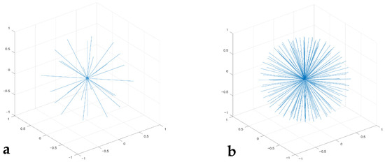
Figure 2.
Initial configuration of the particles in velocity space, where net momentum is zero. The length of the lines defines the velocity of each particle and the orientation shows the direction of motion. These perfect rosettes are evenly distributed in all directions and rotations, which makes determining an initial, null momentum state trivial. The even spacing of the velocity directions will also speed convergence: (a) n = 26; (b) n = 182.
The largest runs (n = 728) had a rosette of 182 directions, with four different velocities per direction. The number of directions was proportionately reduced for runs for n = 182 and 26.
The actual code parallelized the 728 particles on a 64-core processor, for a total of 46,592 particles. Each of the 64 computations was run for 107 collisions. This entire batch of computations was run four times. Every collision was randomly selected based on a continuously recalculated probability matrix of any pair of particles colliding. Collision probability was assumed to be directly proportional to closing speed, which is exact if the number of particles is infinite. The collision probability does not include spatial effects such as distance, as in the classical derivation, since the particles themselves contain no spatial information.
Once the particles were stochastically selected based on their closing speed, the collision contact angle was determined. Contact angle is visualized by imagining a glancing blow or a direct hit. Because position is not part of Maxwell’s or our construction, contact angles cannot depend on the direction of movement of the particles. Instead, contact angles were calculated as follows: Two random numbers were generated and then assigned as an offset distance for the collision, which allowed calculation of the contact angle. If these values failed to generate a collision, this collision offset subroutine was rerun. Once the angle and direction of the collision were determined, the velocities post-collision were calculated using Newtonian mechanics, which conserves both momentum and energy. The velocity matrix was updated, and the process was repeated. In detail, the random number generator was a pseudo-random Mersenne twister set to shuffle its seed. The software uses single precision (16 digits).
4.1.2. Code, Equipment, and Programs Used
Code was written in Matlab. We used a Dell PowerEdge R7525 computational server which consists of dual 2.0/3.3 GHz AMD EPYC 7662 64 core processors, 512 GB of RAM and 12TB of local storage. This server is part of the Planetary Materials Group in the EEPS Department. The commercially available program KalediaGraph was used to graph and analyze the data. Fits are least squares.
4.2. Numerical Results
For each n, we present distributions for the same mean energy because this equals kT times a numerical factor that is independent of n in the one-parameter classical model. Our plotting program has a limit of 400 bins for conversion of the list of velocity components for the particles (i.e., histogram data) to the number of particles as functions of either velocity or energy. Our fits are slightly affected by bin size, but this does not alter the conclusions (Appendix A).
4.2.1. Directional Dependence of Velocities
For each direction and each n, velocities peak at v = 0 and are evenly distributed at positive and negative values, but with scatter (Figure 3). Scatter near the origin stems from no particle having KE = E = 0.
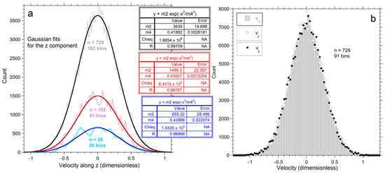
Figure 3.
Results for velocity along each Cartesian direction, after 107 conservative collisions. The average energy is identical for each n explored: (a) Jagged pale curves show binned data. Dark curves show least squares fits to a normal distribution (insets), with n increasing upwards; (b) Directional dependence for velocities for 728 particles, using 91 bins for each direction. The grey histogram shows vx output data. Circles = binned values for vy. Dots = binned values for vz.
All n-values produce nearly Gaussian velocity distributions (Figure 3a). Bin number was selected to give reasonably smooth distributions for each n: See Appendix A for details.
As particle number increases, the histograms become smoother and the fit to a Gaussian improves (Figure 3a, insets). All distributions have a finite upper limit that increases with n, which is quantified in Section 4.2.3. Distributions for the three directional components are nearly equal for 728 particles (Figure 3b). Variations between components decrease as n increases, because the population of each bin increases with n, thereby smoothing the histogram.
Projections of velocity space onto the three orthogonal planes emphasize progressive depopulation of both large and very small velocities as n decreases (Figure 4, Figure 5 and Figure 6). The concentrations of particles is much denser for n =182 than for n = 26, particularly towards the center. Also, each plane appears similar for n = 182, whereas for n = 26 scatter in velocities make the planes appear slightly different. Plots for 728 particles (Figure 6) show very dense coverage towards the center, little difference among orientations, and more regular behavior as velocity increases: hence the smoother histogram in Figure 3 for n = 728.
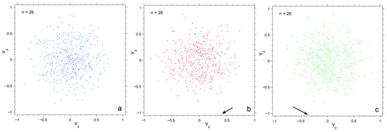
Figure 4.
Projections of the numerical calculation for n = 26 onto three planes in velocity space. Black arrows point to particles with high speed in the various projections. Symbol size is 6 points; (a) The xy plane; (b) The xz plane; (c) The yz plane.
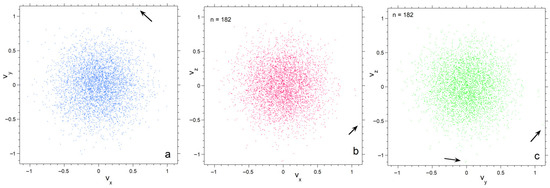
Figure 5.
Projections of the numerical calculation for n = 182 onto three planes in velocity space. Black arrows point to particles with high speeds in the various projections. Symbol size is 3 points; (a) The xy plane; (b) The xy plane; (c) The yz plane.
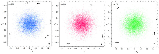
Figure 6.
Projections of the numerical calculation for n = 728 onto three planes in velocity space. Black arrows point to particles. Symbol size is 2 points: (a) The xy plane; (b) The xy plane; (c) The yz plane.
4.2.2. Histograms of Energy
Energy for each particle is obtained by applying Equation (2) to output on its vx, vy and vz components. Numerical results for energy are shown as histograms (Figure 7) with bin sizes chosen to give reasonably smooth distributions for each n. Statistics for the energy histograms (Figure 7a–c, insets) are independent of binning and confirm that <E> is identical for all three examples. As n increases, the histogram becomes wider (greater variance) and reaches higher E, while the mean and cutoff energy also increase.
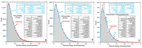
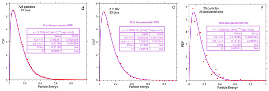
Figure 7.
Kinetic energy distributions: (a–c) Numerical output for each value of n, shown as grey histogram, which is not normalized as indicated by the y-axis scale. The large box shows statistics for each histogram. Red dots = binned values normalized to produce an area of unity. Blue curves show the least-squares fits to the normalized binned data (red dots) to the one-parameter Maxwellian distribution of Equation (7) for each n explored; (d–f) Normalized binned histograms for each value of n. The binned data (red dots) are the same as in the top row, but now the y-axis displays the normalized values. Purple curves and the insets are fits to our proposed two-parameter gamma distribution of Equation (9).
Independent of fitting, the mode, variance, skewedness and kurtosis of the calculated energies depend on n at constant <E>, as shown by the statistics of the histograms (insets in Figure 7a–c). Thus, the numerical calculations refute validity of the classical formulation for small n for which all measures of shape are independent of n. Instead, the relationships are consistent with that of a gamma distribution, Equations (9) and (10). Importantly,
- Variations in the shape of the energy distribution with n are a consequence of heat differing from temperature.
4.2.3. Parameters for Probability Distribution Functions from Fitting Numerical Results
Normalization of the classical function to provide a PDF has masked problems with energy conservation (Section 1). Normalization is required to evaluate representations of statistical data by a continuous function. Thus, comparing our numerical results to the PDFs of Equations (7) and (9) requires binning the histogram data in Figure 7a–c and setting the area under the histogram curves to 1. Effects of bin size are contained in the uncertainties in the fitting coefficients: Appendix A provides further discussion.
Fits to Equations (7) and (9) both improve with n due to smoothing (Figure 7). For each n, our proposed Equation (9) better represents the numerical result than the classical formula, Equation (7). For n = 728, departures from Equation (7) are evident in the extracted parameters. Importantly, fitting to the Maxwell–Boltzmann distribution (the PDF of Equation (7)) provides Θ = kT that varies with n (Figure 7a–c). Thus:
- Fits of the data to Equation (7) refute that the expectation value in F simply equals kT.
- The classical model inadequately describes n near 728 and below.
Figure 8 compares parameters from histogram statistics to fitting coefficients. Simple power laws or linear fits to n are shown because only three values of n were investigated. Both the classical and proposed PDFs overestimate the mean energy, due to their infinite limits (Figure 8a). Both models increasingly depart from the mean energy as n decreases such that the discrepancy for the classical model is greater. For n = 26, the gamma function (PDF*, Equation (9)) fits the numerical results significantly better than the classical model (Figure 7c and Figure 8b).
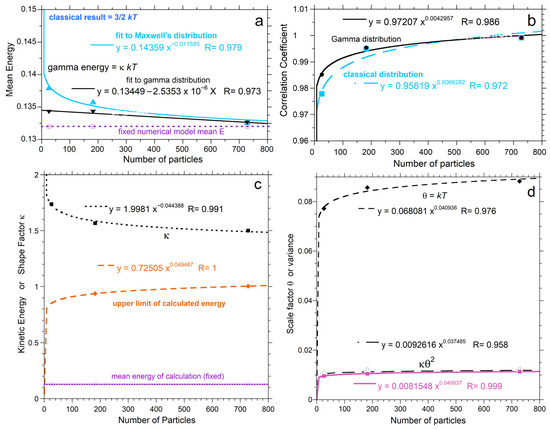
Figure 8.
Dependence of distribution properties on n from fitting the PDFs: (a) Comparison of fits to the classical (blue up-pointing triangles) and proposed (black down-pointing triangles) PDFs. Dashed-dot line = mean energy from the calculations, which is lower because both PDFs extend to infinity. Triangles = <E> from fitting. (b) Comparison of correlation coefficients for fits to the classical (blue squares) and proposed (black circles) PDFs; (c,d) Comparison of parameters, as labeled, from the proposed two-parameter PDF to histogram statistics from the insets of Figure 6a–c, which were not normalized. The upper limit of the calculation (orange diamonds) increases with n, but only weakly, and thus does not extrapolate to infinity as n becomes large. Variance (κ2Θ) from the fit (black) slightly exceeds values from statistics of the numerical calculation (pink) because the gamma distribution extends to infinity.
Figure 8c,d compare histogram statistics to parameters obtained from fits to the proposed PDF of Equation (9). Maximum calculated particle energy approaches unity for n = 728: this corresponds to 1% of the total energy and occurs when the numerical calculations approach the classical distribution. The shape factor κ asymptotes to the immense n result of 3/2, and behaves as expected with n (Section 2.2, last paragraph).
The scaling factor Θ depends on n (Figure 8c,d) because the mean <E> = κΘ = κkT was held constant in the comparisons, and κ depends on n (Equation (11)). Importantly, histogram data in Figure 7 and Figure 8 are based on the numerical results having identical <E> for all n. Thus, Θ = kT depending on n is a consequence of the tail of the PDF extending beyond the maximum calculated velocity. The excess in the PDF becomes more pronounced as n decreases.
Variance obtained from fitting parameters is slightly larger than the statistical variance for the histogram. Both discrepancies arise from the infinite limit of a continuous distribution function. The following points summarize behavior:
- From the various trends, elastic systems exceeding ~1000 particles are represented reasonably by the continuous PDFs with κ = 3/2, although very high speeds are not actually populated, so the mean energy remains overestimated, albeit slightly, as shown in Figure 8.
- The maximum energy at steady-state cannot exceed Etot/6, in view of energy conservation and momentum conservation in three directions, and appears to be less given the results for n = 728, where Emax is close to 1 and Etot is 96.
Comparing PDFs with the same total energy = n<E> would provide the same results as comparing the same <E> because the fitting is performed after normalizing the area under the histogram to unity.
The continuous functions have finite probabilities (finite area) above the maximum E attained at steady-state during the collisions of a finite number of particles, as established numerically here.
- Finite probability for unattainably high energies underlies discrepancies of the classical and proposed models from the numerical results.
4.2.4. Energy Measures and Conservation in Finite n Collections
Several features in the energy histograms are independent of bin size. We show that the distributions uphold total energy and momentum conservation and adhere to no particle being stationary. The cause is ongoing collisions.
Total energy from our numerical calculation is proportional to n since <E> is the same for all three examples. Finite Etotal (heat) and finite n require a cutoff in E. Also,
- No single particle can have E = Etotal, because that case would require all other particles to have E = 0, which prohibits momentum conservation and balance.
Thus, the PDF should equal 0 at Emax < Etotal and beyond. Finite probability should exist for several outliers at speeds up to Emax, which for n = 728 is merely ~1% of Etot. Below, we describe how to ascertain the cutoff in E.
Figure 7c (n = 26) clearly shows these features, where the bump in the histogram (not normalized) near E = 0.67 describes 15 datapoints out of 6656 total; one datapoint falls at E = 0.47, and the remainder with energies <0.45 are well-populated. The even number of datapoints (16) at high E is a consequence of momentum conservation. The total energy of 3.43 = 26<E> cannot be possessed by a single particle. Nor can total energy be divided among 6 moving particles (not datapoints), in which case momentum is conserved in all three physical directions, because this requires 20 particles to be impossibly stationary. However, a few fast particles can exist. Specifically,
- The few datapoints near 0.6785 (0.198Etotal) represent the improbable circumstance of a few fast and many slow particles out of 26, where total energy and total momentum are conserved.
An expanded view (Figure 9b) of the high energy tail for n = 182 in Figure 7b shows that outliers likewise exist for larger n systems. Of the 46,595 datapoints, 12 have E near 0.93 (0.39%Etotal) and 10 have E near 0.82, while the remainder form a continuous distribution below E < 0.7. The fastest particles lie far below Etot = 24.
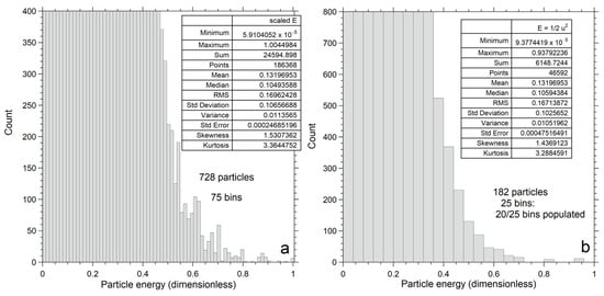
Figure 9.
Expanded views of the kinetic energy histograms in Figure 7a,b, designed to emphasize the outliers. This representation is not normalized, as indicated by the y-axis scales. The large box in each panel shows statistics: (a) Numerical output for n = 728; (b) Numerical output for n = 182.
An expanded view (Figure 9a) of the high energy tail for n = 728 in Figure 7a shows that outliers remain at the highest n numerically explored here. Of the 186,368 datapoints, 6 have E near 1 (0.011Etotal), 3 have E near 0.94, and 32 have E near 0.87, while the remainder form a continuous distribution with E < 0.83. The fastest particles lie far below Etot = 96.
As n in small populations decreases, energies of the fastest particles are increasingly restricted. Consequently, the maximum energy increases strongly with n at low n and then flattens (Figure 8c). The weak dependence of Emax on n at large n exists because we have implicitly assumed that the volume is finite. So, a collection with a large number of particles has more frequent collisions in physical space, which increasingly limits individual particles from attaining high speeds as n increases. High speed outliers become less important to the statistics as n increases due to the frequent collisions providing more reversals. The limit at 10 million collisions is near Emax = 1 for n = 728 (Figure 7a), which is far below the total energy of 96.0738. As n increases, the limit will increase but can never reach the total energy of the system due to energy as well as momentum conservation. Discussion continues in Section 5.2 and Section 6.4.
5. Discussion
Our analytical model shows that the Maxwell–Boltzmann speed distribution, recast in terms of energy [14], is a special case of the gamma distribution family of functions. Other special cases are the exponential distribution, the Erlang distribution, and the chi-squared distribution [26,27].
Our numerical models, exploring conservative collisions in three-dimensional physical space, provide spherically symmetric velocity space, as expected for a non-rotating, non-translating system of elastic particles. Furthermore, our numerical results validate our proposal of a two-parameter (κ and Θ) gamma distribution function as the continuous energy representation. This function and its corresponding PDF (Equation (9)) address that heat and temperature differ, but are related. Evidence includes the following:
- Fitting our numerical results to the RHS of Equation (9) indicates that not only the shape factor (κ), but also the expectation value (Θ) depend on n.
The variable expectation value results from the numerical calculations conserving total energy, whereas continuous PDFs extend to infinity and so do not conserve total energy (see Equation (5) and the Introduction). In other words, the classical formulation provides finite probability for energies exceeding the system energy, whose probabilities must instead be zero. Excesses in the classical distribution are evident in:
- The continuous PDFs begin to fail near E = 0.8, where outliers exist,
- Mismatches exist up to termination near E = 1 for n = 728.
All particles in the system move, a result of the plethora of collisions, which testifies to the unattainability of temperatures equaling absolute zero (Nernst’s statement of the 3rd law). Due to energy conservation, infinite temperature is also unattainable and so a realistic PDF must have some cutoff, depending on the heat-energy supplied to the collection of particles. For details, see Section 4.2.4 and Section 5.3.
5.1. Momentum Conservation, the Lower Limit for n, and Dimensions of Physical Space
Momentum conservation in each of the three orthogonal directions requires at least three pairs of particles. This statement is based on our numerical approach allowing for collisions of particles travelling in any direction (Section 4.1.1). Thus, systems with n below six do not adhere to Maxwell’s assumptions (Section 3.1). The smallest n considered here (=26) exceeds this minimum and reveals consequences of total energy not being conserved in the continuous formulations. A second parameter (κ) besides kT is needed to describe the difference between heat and temperature.
Total momentum is conserved in Maxwell’s construction (Figure 1a,b). The numerical calculations confirm that the classical and proposed PDFs are based on collisions in three-dimensional physical space. How might systems with lower dimensionalities behave?
A one-dimensional line of a finite number of equal mass colliding particles must all possess the same kinetic energy at steady-state due to momentum and energy conservation and because collisions are limited to nearest neighbors. The value for <E> is set by Equation (5) as in the three-dimensional case. The energy distribution function for one-dimensional space is a delta function.
For a two-dimensional plane, the velocity distribution functions should be symmetrical (Gaussian) in x and y coordinates. Because the z-coordinate is irrelevant, the relationship of heat (total energy) with temperature (an average) differs between two- and three-dimensional systems, so their shape factors should differ even if their expectation values do not. Solving for the distribution functions in two-dimensional space is beyond the scope of the present report.
5.2. Incorporating Conservation of Total Energy into F* and PDF*
Our results (e.g., Figure 3, Figure 7, Figure 8 and Figure 9, along with recognizing that no particle can have all or more than the system’s total energy) show the analytical distribution function must be truncated at some finite energy. We sketch two possibilities, recognizing that a high degree of accuracy requires additional numerical computations for more values of n and perhaps more than 107 collisions for very low n systems.
As discussed in Section 4.2.4, the cutoff is near unity for n = 728. Dimensionless E, used here, can be cast as multiples of kT. The RHS of Equation (7) fits the numerical calculation for n = 728 (i.e., κ = 3/2), except for the tail from E = 1 to infinity. Because <E> = 0.13196953, which should be very close to 3/2 kT for large n, then Emax is 11.37 kT, and the total heat energy is 64 kT for n = 728, which nearly matches the Maxwellian result for infinite n. On this basis, we propose the following:
- For very large n, the classical PDF should be likewise truncated at Emax = 11.37 kT, i.e., Emax is ~1% of Etot.
- For small n, the proposed PDF* of Equation (9) should be used, and Emax should be reduced in accord with the fit shown in Figure 8c.
Regarding energy conservation, overestimations associated with applying a continuous distribution for n between ~20 and ~1000 can be addressed using the fits of Figure 8:
kT = 0.068061n0.040936 and κ = 1.9981n−0.44388.
Then, mean energy can either be estimated from using either:
or, alternatively, Equation (9) can be used in a spread sheet up to the limit of E = 0.04692n0.12091.
<E> = 0.13449–2.5353 × 10⁻⁶n,
Upon calculating the mean energies, the total is provided by n<E>. A finite value for heat results, and thus energy, is conserved.
5.3. Beyond Maxwell’s Assumptions: Possible Future Directions
5.3.1. Density Should Affect Collision Probabilities
Volume does not actually enter into the formulation, yet density = volume/n is an important parameter for matter, particularly a gas. Density describes how matter fills any given space, whereas Maxwell’s approach and our generalization thereof describe how energy fills this same space.
The asymptotic trends of F and F* are a consequence of assuming a finite volume in physical space where the collision probability is not affected either by the number of particles in the volume or by the distance between particles. There is no term which allows addressing changes in density or collision probability. Because of this omission, the Maxwell–Boltzmann distribution does not accurately describe either highly compressed gas or highly rarified gas, unless, perhaps, the latter involves immense volumes and large expanses of time. Section 6 continues this discussion, although further investigation is needed.
5.3.2. Alternative Distribution Functions?
The two-parameter gamma distribution reduces to the classical formulation at large n and is a good match to the numerical results up to the maximum energy (Figure 7d–f). It is unlikely that any other analytical function extending to infinity meets both criteria. However, a three-parameter function intended to address collision probability depending on particle number may be worth pursuing, to address the concerns mentioned in Section 5.3.1. We do not suggest incorporating volume, as this can be estimated from the speed distribution, if probability is incorporated, as this relates to time.
An analytical form terminating a finite energy (without specifying this energy) is desirable. Whether this is possible is an open question of long-standing interest in statistics: See Section 2.3 and References [28,29].
5.3.3. Hard Elastic Sphere Assumption
Assuming elasticity neglects that collisions deform atoms, which consumes some energy of the translation, thereby producing losses and affecting energy distributions [31] (chapter 5). However, under steady-state conditions, energy losses are compensated by the influx of heat, which state of quasi-equilibrium describes many situations, including colliding gas particles. Transport properties are a response to disequilibrium conditions. Local equilibrium conditions are not met, even during steady-state where the flow of heat depends on space but not time [32]. Transport measurements probe the dynamic response of matter. This circumstance is evident in gas transport data systematically diverging from the classical kinetic theory of gas (see chapter 5 in [31]).
Due to inelasticity, whereby energy is lost, isothermal conditions require heat input to balance heat output. Whether the energy distribution for idealized elastic collision applies to an inelastically colliding gas depends on how much energy is lost in the collisions. If the losses are proportional to the velocities squared, the mathematical forms of the classical and proposed PDFs should be unchanged, although the cutoff would be affected by the fractional loss. Further theoretical and numerical investigation is warranted to address inelasticity and its possible dependence on velocity.
6. Implications
6.1. The Equipartition Theorem
Due to the focus on speed, which is a scalar, the effects of momentum conservation occurring during each and every collision went unrecognized. Our numerical results (Section 4.2) show that momentum and energy conserving individual collisions in a non-translating system provide equal shapes in the three Cartesian directions. The importance of the Virial Theorem [15,16] to the n particle system, which forms a bound state, has also gone unrecognized. The Virial Theorem and symmetry of Maxwell’s velocity space requires KE be identical in the three orthogonal restrictions (Section 3.4).
These oversights lead to the proposal of the energy equipartition theorem between translations and rotations by Maxwell [4,5] and then between any type of thermal motion by Boltzmann [33]. Neither proposal is needed to explain monatomic gas. Simple gases diverge somewhat from equipartitioning [31] (Table 5.1 therein), so the historic equipartition theorem is not supported by modern data. Earlier, a correct statement was given by Waterston in an 1851 conference abstract [34] (his Appendix II) where he considered the gas to consist entirely of translating particles and collisional exchanges between particles to be regulated by mass [35]. Waterston provided Equation (3), but without numerical factors or defining the proportionality constant, k. Waterston noted momentum conservation of each collision but discussed neither the directional dependence of velocity nor motion types other than translations.
Extending the equipartition theorem to other types of motion than translatory is not supported by our findings or data (e.g., [31] (Chapter 5)). Instead of unrestricted equipartitioning of energy amongst various possibilities, a correct description requires considering how energy would be converted from one form of thermal motion to another. Importantly, the Virial Theorem holds separately for each different type of force acting in (or on) a system due to various energy exchanges being governed by different physical laws [16]. This caveat should also be evident from Equation (12, RHS), which is the product of the scale length of the action with the specific force creating the motion. For additional caveats pertaining to astronomical research, see [16].
6.2. Energy Conservation Is Important at Low Temperature and Low Density
Physical space neither explicitly enters into Maxwell’s construction, nor into our statistical model, nor into our numerical computations. However, collisions occur within some distance, which is defined by the product of velocity with time. The cutoff in energy means that velocity is likewise capped and that a characteristic distance also describes the collisions within a certain span of time. Thus, some physical volume describes the colliding particles at any given temperature. On this basis, a large number of particles in any given volume must collide more frequently than a small number of particles in that same volume. As long as interaction times are short compared to travel times, multiple particles simultaneously colliding is not expected. Instead, the frequency of collisions should increase. Collision cross-sections varying with n have implications for extreme environmental conditions. Two examples merit mentioning:
Rarefied and/or cold environments require a long time to achieve steady-state (quasi-equilibrium). Long times are linked to cold particles being sluggish and/or large distances between particles limiting collision probabilities. Thus, if one particle is energized greatly, it could reach the limits of the relevant volume before its motion is reversed, and its energy is exchanged with another particle. Very highly energized particles can escape the bound state, which is analogous to gas on the surface of a planet having an escape velocity, e.g., [36] (pp. 282–285). For a perturbation to change the temperature (a property of the collection), it must affect the velocities of many particles within a reasonably short time scale. The combination of cold and rarefied conditions in space are resistant to energy perturbations (e.g., receipt of radiation) over short time scales.
In compressed, high-density gas, the particles collide more frequently. Particles interfering with each other restrict the distances travelled. The upper limit on energy would be reduced. This response can be understood by considering solidification, where large-scale particle translations transform into small-scale vibrational modes. Thus, the statistical distribution representing particles in a gas needs modification to incorporate the effect of very high density, prior to solidification.
These examples illustrate that the distribution functions explored analytically and numerically here are idealizations. The implicit limitations need to be considered when addressing extreme conditions. The examples presented above lead us to propose that a third parameter is needed for a speed (energy) distribution function. Collision probability depending on n was suggested in Section 5.3.2. Further exploration is beyond the scope of this report.
6.3. Relevance to Space and Cosmology
Vast regions in space (interstellar and intergalactic media) have hydrogen atoms separated by >1 m. Collision probabilities are low in such rarefied media. Low T over most the universe, excepting stars or star concentrations, are inferred for the densest astronomical gassy media known, those of molecular clouds at 4 to 20 K [37].
Postulated high temperatures of certain intergalactic media rest on observations of absorption spectra. Such electronic transitions are stimulated by high-energy light in the ultraviolet (UV) spectral region, and represent an excited state of the atom, per laboratory optical spectroscopic measurements [38]. Stimulation of electronic transitions by light will negligibly alter the velocity of the cation hosting the electron due to mass differences: This is known as the Born–Oppenheimer approximation [39]. The translational velocity of the whole atom being connected with thermal energy is the heart of the kinetic theory of gas and underlies the energy distribution functions discussed here.
Atoms with excited electrons are not in thermal equilibrium with their neighbors until collisions occur. If relaxation of the electronic excitation occurs over a shorter time scale than that of the collisions, the UV energy is not redistributed among the population. This situation occurs even in dense matter (e.g., [40,41]).
Absorptions of UV light (or other radiation) by ions in space do not indicate temperature because T is a statistical measure of a collection. Thus, the warm–hot medium hypothesis for conditions in intergalactic media lacks a firm physical basis on several counts: also see [20].
Our proposed gamma distribution function and numerical results can be used to explore conditions describing steady-state in the huge expanses of space, which are important regions to astrophysical research. Quasi-equilibrium is possible because times are large.
6.4. Relativistic Speeds Require Millions of Degrees
Speeds are estimated here for a gas of atomic H with n > 1000, where the classical mean of 1.5 kT applies. Total energy of any system (heat) is finite. A system with very large n thus has particles with less energy and a lower average (temperature) compared to a system with modest n, i.e., 728 as investigated here. Energy and momentum conservation, along with the absence of stationary particles, limit Emax to ~1 (~1% of Etot) beyond n~1000.
Our non-dimensional calculations use <E> = 0.132 for all cases. Because Emax is very close to unity for large systems:
From our numerical calculations, temperatures of ~5 × 10¹¹ K are needed for fast H atoms in a finite n gas to reach light-speed. This T-value exceeds the immense temperatures attributed to gas in intergalactic regions of space [20] by five orders of magnitude. Specifically, T~106 K estimated from UV absorptions would contain particles with speeds below 0.14% that of light.
Thus, a relativistic correction is not needed to describe gas bodies under laboratory conditions and would insignificantly affect astronomical media in view of energy conservation. Problems with the non-conservative, infinite n model are discussed in the Introduction.
Author Contributions
E.M.C.: originated the concept and developed and performed numerical modelling. A.M.H.: developed the analytical analysis—writing original draft (lead). All other tasks were equally shared. All authors have read and agreed to the published version of the manuscript.
Funding
This research was partially supported by National Science Foundation, grant number EAR-2122296.
Data Availability Statement
Upon acceptance, numerical results will be deposited and are openly available in perpetuity at https://epsc.wustl.edu/~hofmeist/thermal_data/ (accessed on 18 August 2025), reference number 2024SpeedDistribution.
Acknowledgments
We thank B. Jolliff and H. Chou at Washington University for access to supercomputing facilities.
Conflicts of Interest
Author Everett M. Criss was employed by the company General Dynamics Ordinance and Tactical Systems. The remaining author declares that the research was conducted in the absence of any commercial or financial relationships that could be construed as a potential conflict of interest.
Appendix A. Effect of Bin Size on Fits to PDFs
We focus on small n because bin size negligibly affected results for n = 728, for which the histograms are well-populated and smooth (Figure 7). Bin size slightly affects parameters from fitting the distributions for small n but does not change the findings in Section 4.2, as follows.
For n = 26, one particle per bin (i.e., 26 bins) is the most reasonable choice and was used in Figure 7. For n = 728, 75 bins gave a smooth distribution (~10 particles per bin): little difference was seen in the fits for more and fewer bins (not shown in the figures). We used 50 bins for n = 182 in fitting (Figure 7b,e), because this number provided ~4 particles per bin which is intermediate to the binning of numerical results for n = 26 and n = 728 (Figure 7), and yielded an intermediate amount of scattering. Because choices in binning are limited for n = 26, and the smoothness of curves for n = 728 means that bin size is likely immaterial, we now explore the effect of varying bin size for n = 182.
Figure A1 shows additional fits to our proposed gamma distribution. More bins (smaller bin size) increase the scatter at constant n, so the fits are less certain. Figure A1 shows that the fit to our proposed PDF of Equation (9) improves with increased smoothing provided by fewer bins. The shape parameter is affected more than the expectation value, but given fit uncertainties shown in the insets, results are independent of bin size.

Figure A1.
Effect of bin size, as labeled, for n = 182. Red dots show the top of the bins. Fits (purple curves) are to the proposed two-parameter PDF. Fitting parameters are given in the boxes.
Figure A1.
Effect of bin size, as labeled, for n = 182. Red dots show the top of the bins. Fits (purple curves) are to the proposed two-parameter PDF. Fitting parameters are given in the boxes.

Figure A2 shows the same number of bins as in the various panels of Figure A1 for n = 182, but instead with a fit to the classical PDF of Equation (7). For bins of 25, 50, and 91, our proposed PDF better fits the numerical results. For the noisy result at 200 bins, both fits show a similar mismatch.

Figure A2.
Calculations for 182 particles, binned as labeled (red dots), and fits (various blue curves) to the classical PDF. Fitting parameters are given in the boxes.
Figure A2.
Calculations for 182 particles, binned as labeled (red dots), and fits (various blue curves) to the classical PDF. Fitting parameters are given in the boxes.

Figure A3 shows that bin size does not change the relationship between the parameters from the classical and gamma function fits. The greater noise for a large number of bins affects the two parameters extracted from fits to the gamma function more, but the mean energy is less affected. Trade-offs in fitting are involved. Again, dependence of parameters on n for the gamma function are expected, whereas fits to the classical function should be independent of particle number.


References
- Reif, F. Fundamentals of Statistical and Thermal Physics; McGraw-Hill Book, Co.: St. Louis, MO, USA, 1965. [Google Scholar]
- Isihara, A. Statistical Physics; Academic Press: New York, New York, USA, 1971. [Google Scholar]
- Gyenis, B. Maxwell and the normal distribution: A colored story of probability, independence, and tendency towards equilibrium. Studies Hist. Philos. Modern Phys. 2017, 57, 53–65. [Google Scholar] [CrossRef]
- Maxwell, J.C. Illustrations of the dynamical theory of gases. Part I. On the motions and collisions of perfectly elastic spheres. Lond. Edinb. Dublin Philos. Mag. J. Sci. 1860, 19, 19–32. [Google Scholar] [CrossRef]
- Maxwell, J.C. Illustrations of the dynamical theory of gases. Part II. On the process of diffusion of two or more kinds of moving particles among one another. Lond. Edinb. Dublin Philos. Mag. J. Sci 1860, 120, 21–37. [Google Scholar] [CrossRef]
- Boltzmann, L. Weitere studien über das Wärmegleichgewicht unter Gasmolekülen. Sitz. Kais. Akad. Wiss. Wien Mathemat.-Naturwissenschaft. Cl. 1872, 66, 275–370. [Google Scholar]
- Boltzmann, L. Über die Beziehung zwischen dem zweiten Hauptsatz der mechanischen Wärmetheorie und der Wahrscheinlichkeitsrechnung respektive den Sätzen über das Wärmegleichgewicht. Sitz. Kais. Akad. Wiss. Wien Mathemat.-Naturwissenschaft. Cl. 1877, 76, 373–435. [Google Scholar]
- Sharp, K.; Matschinsky, F. Translation of Ludwig Boltzmann’s Paper “On the Relationship between the Second Fundamental Theorem of the Mechanical Theory of Heat and Probability Calculations Regarding the Conditions for Thermal Equilibrium”. Entropy 2015, 17, 1971. [Google Scholar] [CrossRef]
- Krall, N.A.; Trivelpiece, A.W. Principles of Plasma Physics; San Francisco Press: San Francisco, CA, USA, 1986. [Google Scholar]
- Zhigilei, L.V.; Garrison, B.J. Velocity distributions of molecules ejected in laser ablation. Appl. Phys. Lett. 1986, 71, 551–553. [Google Scholar] [CrossRef]
- Binette, L.; Matadamas, R.; Hägele, G.F.; Nicholls, D.C.; Peña-Guerrero, M.Á.; Morisset, C.; Rodríguez-González, A. Discrepancies between the [O III] and [S III] temperatures in H II regions. Astron. Astrophys. 2012, 547, A29. [Google Scholar] [CrossRef]
- He, J.J.; Zhang, L.Y.; Hou, S.Q.; Xu, S.W. Re-examination of constraints on the Maxwell-Boltzmann distribution by Helioseismology. Chin. Phys. C 2013, 37, 104001. [Google Scholar] [CrossRef]
- Kapil, V.; Cuzzocrea, A.; Ceriotti, M. Anisotropy of the proton momentum distribution in water. J. Phys. Chem. B 2018, 122, 6048–6054. [Google Scholar] [CrossRef]
- Maxwell–Boltzmann Distribution. Available online: https://en.wikipedia.org/wiki/Maxwell%E2%80%93Boltzmann_distribution (accessed on 21 February 2025).
- Clausius, R. Über einen auf die Wärme anwendbaren mechanischen Satz (on a mechanical theorem applicable to heat). Annalen der Physik 1870, 217, 124–130, English Translation in Phil. Mag. 1870, 40, 122–127. [Google Scholar] [CrossRef]
- Hofmeister, A.M.; Criss, R.E. Spatial and symmetry constraints as the basis of the virial theorem and astrophysical implications. Can. J. Phys. 2016, 94, 380–388. [Google Scholar] [CrossRef]
- Halliday, D.; Resnick, R. Physics; John Wiley and Son: New York, NY, USA, 1966. [Google Scholar]
- Johnson, N.L.; Kemp, A.W.; Kotz, S. Univariate Discrete Distributions, 3rd ed.; John Wiley & Sons, Inc.: New York, NY, US, 2005; pp. 156–207. [Google Scholar]
- Falk, M.; Hüsler, J.; Reiss, R.D. Laws of Small Numbers: Extremes and Rare Events; Springer Science & Business Media: Berlin, Germany, 2010. [Google Scholar]
- Reeves, J.; Done, C.; Pounds, K.; Terashima, Y.; Hayashida, K.; Anabuki, N.; Uchino, M.; Turner, M. On why the iron K-shell absorption in AGN is not a signature of the local warm/hot intergalactic medium. Mon. Not. R. Astron. Soc. 2008, 385, L108–L112. [Google Scholar] [CrossRef]
- Wijers, N.A.; Schaye, J.; Oppenheimer, B.D. The warm-hot circumgalactic medium around EAGLE-simulation galaxies and its detection prospects with X-ray and UV line absorption. Mon. Not. R. Ast. Soc. 2020, 498, 574–598. [Google Scholar] [CrossRef]
- Truesdell, C. The Tragicomical History of Thermodynamics; Springer: New York, NY, USA, 1980. [Google Scholar]
- Hofmeister, A.M.; Criss, E.M.; Criss, R.E. Thermodynamic relationships for perfectly elastic solids undergoing steady-state heat flow. Materials 2022, 15, 2638. [Google Scholar] [CrossRef]
- Weaver, C.G. In praise of Clausius entropy: Reassessing the foundations of Boltzmannian statistical mechanics. Found. Phys. 2021, 51, 59. [Google Scholar] [CrossRef]
- Expected Value. Available online: https://en.wikipedia.org/wiki/Expected_value (accessed on 2 May 2025).
- Gamma Distribution. Available online: https://en.wikipedia.org/wiki/Gamma_distribution (accessed on 10 February 2024).
- Kapadia, S.; Chen, W.; Moyé, L. Mathematical Statistics with Applications; Chapman and Hall/CRC Press, Taylor and Francis Group LLC: Boca Raton, FL, USA, 2005; ISBN 0-8247-5400-X. [Google Scholar]
- Erlang, A.K. Probability and telephone calls. Nyt Tidsskr Mat Series B 1909, 20, 33–39. [Google Scholar]
- Beta Distribution. Available online: https://en.wikipedia.org/wiki/Beta_distribution (accessed on 2 May 2025).
- Clausius, R. On the mean length of the paths described by the separate molecules of gaseous bodies on the occurrence of the molecular motion: Together with some other remarks upon the mechanical theory of heat. Lond. Edinb. Dublin Philos. Mag. J. Sci. 1859, 17, 81–91. [Google Scholar] [CrossRef]
- Hofmeister, A.M. Measurements, Mechanisms, and Models of Heat Transport; Elsevier: Amsterdam, The Netherlands, 2019; Chapter 5. [Google Scholar]
- Lavenda, B.H. Thermodynamics of Irreversible Processes; Halsted (Wiley): New York, NY, USA, 1978. [Google Scholar]
- Boltzmann, L. Über die Natur der Gasmoleküle (On the nature of gas molecules). Wien. Berichte 1876, 74, 553–560. (In German) [Google Scholar]
- Waterston, J.J.; Strutt, J.W.I. On the physics of media that are composed of free and perfectly elastic molecules in a state of motion. Philos. Trans. R. Soc. London 1892, 183, 1–79. [Google Scholar]
- Brush, S.G. John James Waterston and the kinetic theory of gases. Am. Scien. 1961, 49, 202–214. [Google Scholar]
- Criss, R.E.; Hofmeister, A.M. Thermal history of the terrestrial planets. In Heat Transport and Energetics of the Earth and Rocky Planets; Hofmeister, A.M., Ed.; Elsevier: Amsterdam, The Netherlands, 2020; pp. 267–296. [Google Scholar]
- Bergin, E.A.; Tafalla, M. Cold dark clouds: The initial conditions for star formation. Ann. Rev. Astron. Astrophys. 2007, 45, 339–396. [Google Scholar] [CrossRef]
- Parson, W.W.; Burda, C. Modern Optical Spectroscopy: From Fundamentals to Applications in Chemistry, Biochemistry and Biophysics; Springer: Berlin/Heidelberg, Germany, 2023. [Google Scholar]
- Born, M.; Oppenheimer, J.R. Zur Quantentheorie der Molekeln. Ann. Phys. 1927, 389, 457–484. [Google Scholar] [CrossRef]
- Schoenlein, R.W.; Lin, W.Z.; Fujimoto, J.G.; Eesley, G.L. Femtosecond studies of nonequilibrium electronic processes in metals. Phys. Rev. Lett. 1987, 58, 1680–1683. [Google Scholar] [CrossRef]
- Aeschlimann, M.; Bauer, M.; Pawlik, S.; Knorren, R.; Bouzerar, G.; Bennemann, K.H. Transport and dynamics of optically excited electrons in metals. Appl. Phys. A 2000, 71, 485–491. [Google Scholar] [CrossRef]


Disclaimer/Publisher’s Note: The statements, opinions and data contained in all publications are solely those of the individual author(s) and contributor(s) and not of MDPI and/or the editor(s). MDPI and/or the editor(s) disclaim responsibility for any injury to people or property resulting from any ideas, methods, instructions or products referred to in the content. |
© 2025 by the authors. Licensee MDPI, Basel, Switzerland. This article is an open access article distributed under the terms and conditions of the Creative Commons Attribution (CC BY) license (https://creativecommons.org/licenses/by/4.0/).