Variability of the Spreading of the Patos Lagoon Plume Using Numerical Drifters

Abstract

The Patos Lagoon coastal plume is a small-scale outflow that is strongly controlled by meteorological tides. However, the riverine discharge of the lagoon is subject to high decadal variability. Hence, the discharge amount alters the scale of this coastal plume and its effects over the inner shelf environment. This study uses hydrodynamic simulations and a Lagrangian model to estimate the spreading of the plume under two different discharge conditions.Through scale parameters, we characterized the contrasts of the plume structure between high discharge and low discharge conditions. During a strong discharge regime, the width and thickness of the plume are enhanced, and the inertial processes increase against the frictional effect of the wind. The consequences of these differences include higher values of alongshore and cross-shore spreading of the drifters for the strong discharge regime. These findings indicate that under similar wind conditions, different amounts of riverine discharges alter the extent to which the material delivered by the plume can spread over the inner continental shelf.

1. Introduction

A considerable amount of the global precipitation over the continents is delivered by rivers to the oceans through coastal plumes [1]. The transport and mixing of the material delivered by rivers to the deep ocean is strongly influenced by the plume structure [2]. Coastal plumes have diverse scales and structures; large-scale plumes can extend beyond the continental shelf and affect mesoscale processes due to superficial stratification [3], while small scale plumes have a significant role on the transport of sediments and organic matter at the inner shelf and coastal zones due to mixing and straining processes [4,5,6]. The diversity of coastal plumes is more extensively studied by the use of numerical simulations, thus enabling the characterization of the main physical forcings of plume dynamics [7].

In the inner shelf environment, the variability of the spreading of small coastal plumes is subjected to ambient currents, tides, Coriolis force, wind and river discharge [8,9]. Winds and Coriolis parameter are major mechanisms on the far-field (inner and outer shelf) [10], while in the near-field (adjacent region to the river mouth), buoyancy and tides are more important [11]. The near-field has a supercritical flow condition and is where the bulk turbulent dissipation and dilution of the plume occurs [12,13]. Turbulent dissipation is linked to the lateral spreading of plumes, consequently modifying plume thickness along the plume field [14]. An experimental study conducted by [13] showed that lateral spreading does not impact local mixing, but spreading can increase the area of the subsurface interface, which is responsible for enhancing mixing processes. Therefore, the lateral spreading is a important quantity to determine the extent of the riverine material delivered by a coastal plume to the adjacencies of its near-field.

For a small coastal plumes the structure is determined by the outflow jet of the riverine discharge [15], the extent of sediment and other organic compounds can also be modulate by wind disturbances [16,17]. Oscillations of atmospheric systems are associated with precipitation and the wind field, which control the variability of the plume field [18]. Precipitation is linked to riverine discharge and directly controls plume width in addition to the amounts of sediments transported seaward [4,5]. Wind direction and intensity induce upwelling or downwelling, which widen or narrow the plume, respectively, [19,20]. For a small scale plume, ref. [21] showed an interplay between the wind and buoyancy forcing mechanisms, which the plume circulation behavior is associated with the dominance of wind-induced currents over the baroclinic pressure gradient. As the baroclinic pressure develops from the density gradient created by the amount of the riverine discharge, the circulation of the plume is strongly affected by changes in the riverine discharge. Additionally, ref. [22] highlight how the stratification and circulation of small plume is affected by the wind stress. Estimates of coastal plume spreading generally are studied by using numerical hydrodynamic simulations, field measurements and remote sensing [23], although in situ investigations are limited by higher spatial plume variability in addition to the costs involved in cruise campaigns [24]. Hence, the circulations of coastal plumes are mostly investigated by numerical models [25].

The goal of this study was to measure how the outflow of Patos Lagoon effect the spreading of simulated drifters released at the nearfield of the coastal plume, showing how changes in the parameters of the plume affects the advection simulated drifters released in two simulations with high and low discharge regimes. This paper is organized as follows. Section 2 describes the numerical model, including numerical experiments and an explanation of the plume scale parameters. The results and discussion are presented in Section 3. Finally, Section 4 presents the main conclusions of this work.

Study Area

The Patos Lagoon coastal plume presented in Figure 1 is the second major source of low salinity gradients on the inner sector of Southern Brazilian Shelf, which is embedded by the La Plata River plume which reach the bottom of the middle sector of the continental shelf [26,27]. The plume is formed by the freshwater discharge of the entire lagoon system that passes through a 4-km-long by 600-m-wide jetty mouth into the coastal zone, capable to spread 30 km away from the inlet mouth. Its flow is mainly controlled by meteorological tides, in opposition to its astronomical tide range of only 0.50 m, being subject to progressive dumping across the estuary’s channel [28,29].

The meteorological tide mechanism relies on northeast and southeast winds related to the high pressure center of the South Atlantic and the passage of cold fronts, respectively. In ebb conditions, the seawater intrusion could reach 40 km towards the estuary’s interior; during flood conditions, the Patos Lagoon plume can extend to an area of 700 km ${}^2$ offshore [30]. Field and Light Detection Furthermore, Ranging (LiDAR) measurements conducted by [31] showed the presence of four distinct regions: I. an unstratified freshwater region at the estuarine site, II. a liftoff region of the plume marked by bottom stratification along the jetties, III. a region with superficial freshwater stratification and IV. an exterior region marked by uniform seawater stratification, where the plume water is significantly diluted. In this work, the near-field zone refers to the region III and the far-field refers to the region IV.

Prior studies focused mainly on numerical simulations concerned with the investigation of the lagoon and estuarine 2D-hydrodynamics, where the wind and riverine discharge dominate the water exchange between the lagoon and external sea [32,33]. The roles of earth rotation, winds, tides and river discharge on the Patos Lagoon plume circulation were studied by [10] using a 3D-hydrodynamics approach, where the first variability mode (70%) is characterized by the plume propagation southward. Regarding processes such as straining and advection, vertical advection is the major process driving the stratification cycles at that site [6]. Sediment dispersions delivered by the plume are influenced by a cyclonic eddy downstream of the inlet (contrary to the Kelvin waves’ propagation), while at upstream, the winds and coastal currents are responsible for dispersion along and cross-shore [34].

2. Material and Methods

2.1. Hydrodynamic Model and Lagrangian Module

The hydrodynamic simulations were performed using the TELEMAC-3D three-dimensional model from the open TELEMAC-MASCARET suite, version v6p3 (http://www.opentelemac.org/, accessed on 6 April 2018). The TELEMAC-3D model solves the Navier–Stokes equations by considering local variations in the free surface for each time step for an incompressible fluid, assuming the Boussinesq approximation [35]. Our simulations were performed using the TELEMAC-3D non-hydrostatic module, where the continuity step accounts for the dynamic pressure gradient in order to obtain the vertical velocity. $\kappa -ϵ$ is parametrized for the turbulence model, which is represented by a set of differential equations for evaluation of the turbulent kinetic energy production and turbulent dissipation. The non-hydrostatic Navier–Stokes equation solved by the TELEMAC-3D and the equation for the pressure field are presented in Equations (1) and (2), respectively:

$$\frac{\partial \overrightarrow{U}}{\partial t}+\overrightarrow{U}▽·\left(\overrightarrow{U}\right)=-\frac{1}{\rho }▽p+g+\upsilon {▽}^2\overrightarrow{U}+F$$

(1)

$\overrightarrow{U}$ are the velocity vector, p is the pressure for a non-hydrostatic field, $\rho$ is the density, $\upsilon$ is the difusity coefficient and F is the sources terms, which includes terms denoting the wind, the Coriolis force and the bottom friction. These characteristics make this 3D model able to capture the main features of coastal plumes due the reproduction of vertical recirculation cells and stratification effects assuming the non-hydrostatic pressure distribution.

The numerical domain is constructed by an unstructured mesh solved by finite elements methods, with spatial discretization varying between 10,000 m at the oceanic boundary to 15 m around the Patos Lagoon jetties. Bathymetry information is comprised of nautical charts from the National Navy for the lagoon and estuarine region, the data for the continental shelf were provided by the Exclusive Economic Zone National Assessment Program (ReviZEE), and data from the GEBCO were used for the deep ocean (Figure 1).

The Lagrangian module used in this work consists of passive drifters advected by the velocity field computed by TELEMAC-3D, similar to the used by [36]. The drifters were initialized at the inlet with null velocity, and the evolution of the drifters’ trajectories was performed for each time step. No diffusion coefficient was used; the advection of the drifters is based on the interpolation of the velocities of the surrounding nodes of the computational mesh over each drifter, similar to the study reported by [37].

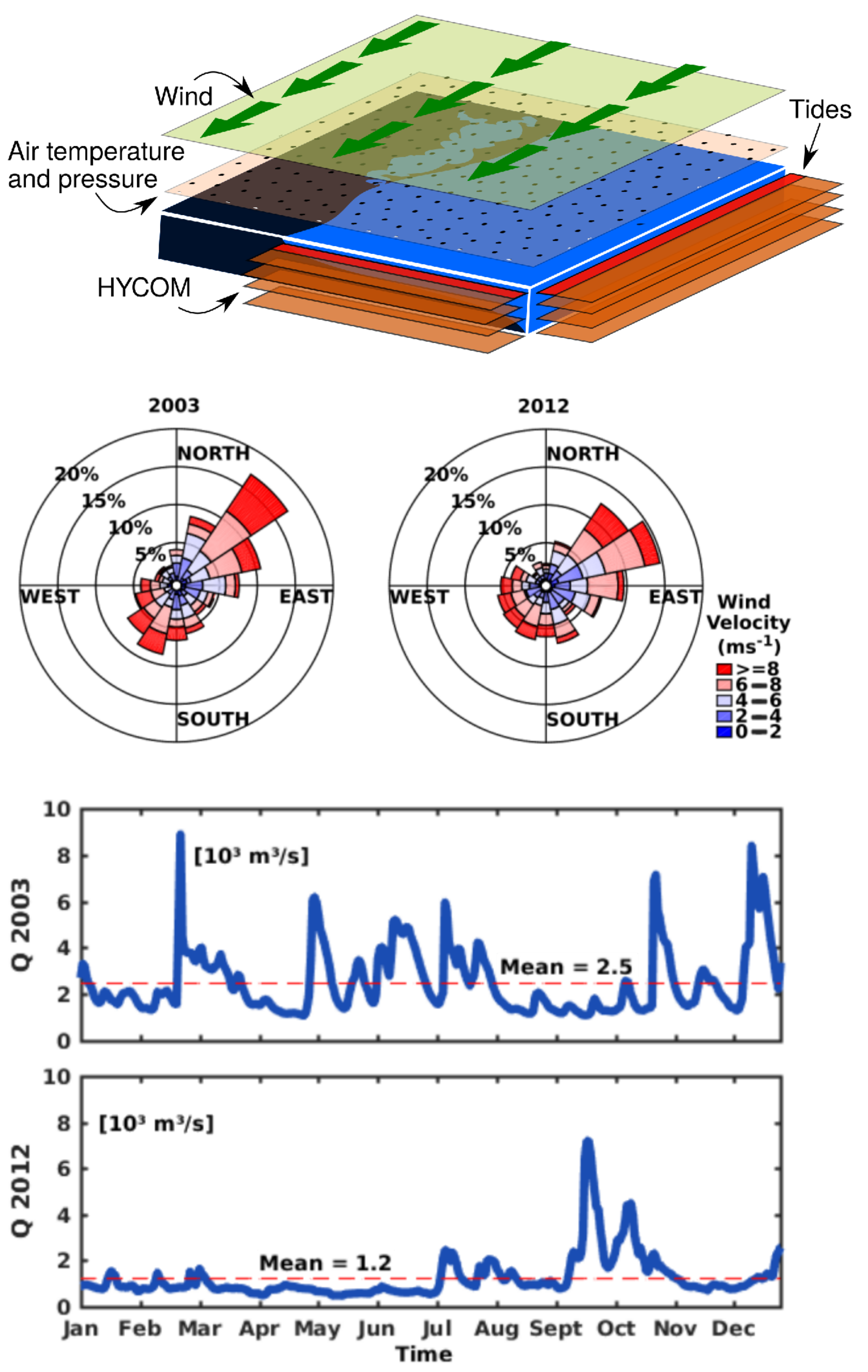
2.2. Boundary Conditions

The simulations were forced at the lagoon interior by riverine discharge, at the oceanic boundary by oceanic tides and currents and its thermohaline properties derived from global oceanic models and at the surface by atmospheric data from reanalysis products. The upper panel of Figure 2 summarizes the application of boundary conditions in the simulation domain.

At the interior of the lagoon, the daily discharge of the three major rivers—the Guaíba, the Camaquã and the São Gonçalo rivers—were prescribed. These data were acquired from the Brazilian National Water Agency (ANA) (http://www3.ana.gov.br/, accessed on 6 April 2018). At oceanic boundaries, velocities, temperatures and salinities from the Hybrid Coordinate Model(GOFS 3.1: 41-layer HYCOM + NCODA Global 1/12 ° Analysis— [38]) were interpolated to the 15 sigma levels of our domain. Additionally, at the oceanic limit, tide constituents from the Tidal Prediction Software from Oregon State University (OSUTPS—[39]) were imposed [40]. Wind velocity, air temperature and air pressure data from the ERA-Interim reanalysis product (ECMWF—[41]) were imposed on the entire surface of our domain.

Three simulations were performed: one from January to February of 2011 for validation, and two for the years 2003 and 2012 as case studies. The middle panel of Figure 2 shows the wind rose, and the lower panel shows the total discharge imposed on the case studies. Both years have similar frequencies regarding wind intensity and direction, with the prevalence of northeast and southwest winds reaching velocities >6 ms ${}^{-1}$. Year 2003 has a mean discharge of 2.5 × 10 ${}^3$ m ${}^3$ s ${}^{-1}$, with peaks >6 × 10 ${}^3$ m ${}^3$ s ${}^{-1}$ distributed throughout the year, while 2012 presents a mean discharge of 1.2 × 10 ${}^3$ m ${}^3$ s ${}^{-1}$, with discharge peaks occurring by September.

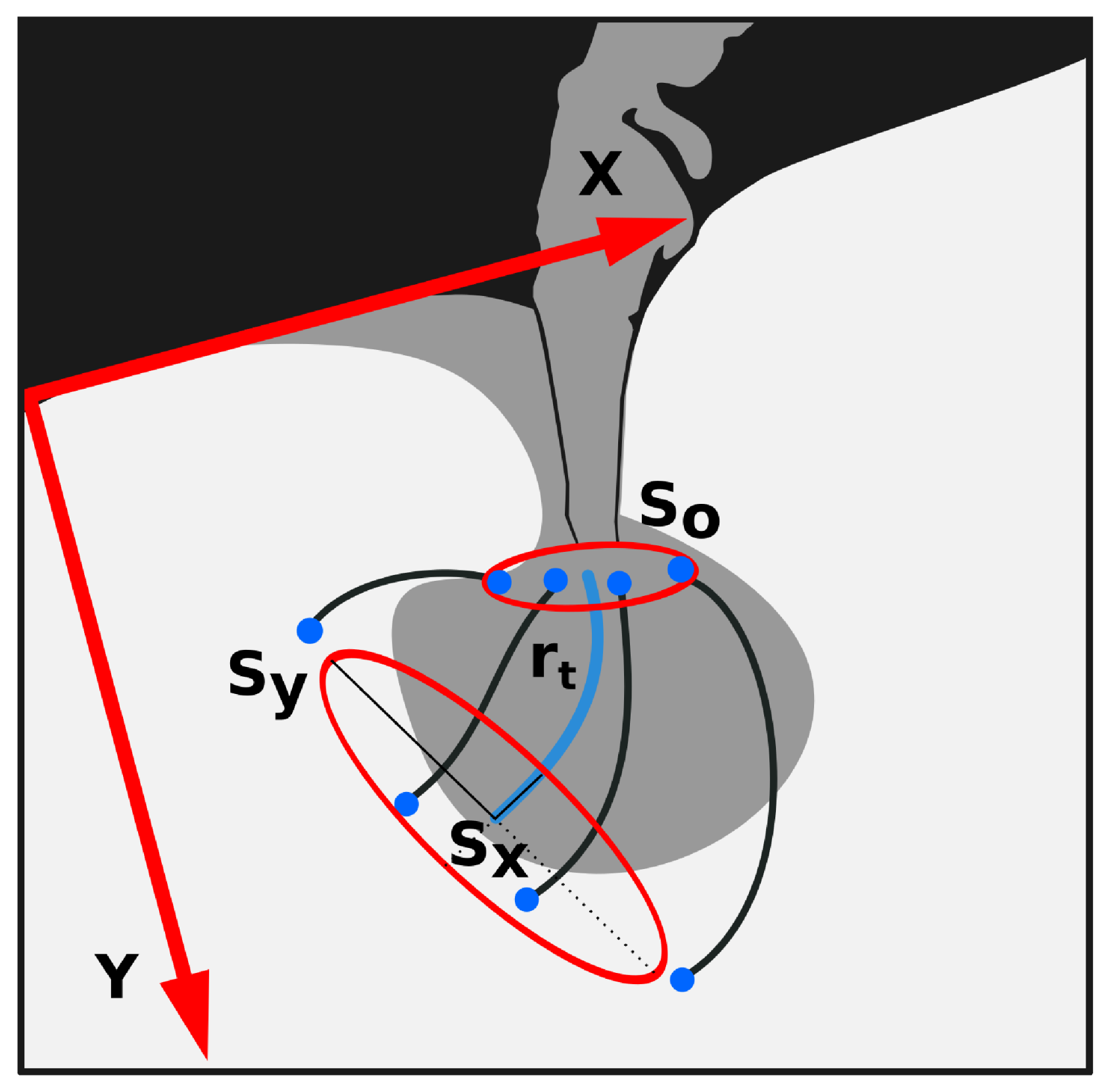
2.3. Drifters’ Spreading Metrics

Estimates of the spreading field from the Patos Lagoon coastal plume were made using the results of trajectories for simulated inert drifters released at the inlet mouth. The drifters were initialized 200 m from the inlet, where 15 drifters was spaced radially around the jetties. The drifters was released daily along each year of 2003 and 2012. The drifters were advected through the velocity field of the hydrodynamic model, and each drift represents an inert particle in the flow without the use of diffusivity coefficients.

Metrics for the spreading of the coastal plume were constructed using the standard deviation of the positions along the center of mass in the alongshore and cross-shore axes, similar to the approach proposed by [42]. The center of mass ${\overrightarrow{r}}_t$ (with components $\overrightarrow{r_x}$ and $\overrightarrow{r_y}$) for each cluster was obtained by averaging the positions of all the drifters for each time-step. The drifters’ positions’ standard deviations were calculated in reference to the coastline, as shown in Figure 3. The alongshore direction is referenced to the x-axis, the cross-shore direction is referenced to the y-axis, and the spreading around the center of mass for each direction was calculated by Equations (2) and (3).

$$S_x=\sqrt{\frac{{\displaystyle \sum _{i=1}^N}(x_i-\overrightarrow{r_x})}{N-1}}$$

(2)

$$S_y=\sqrt{\frac{{\displaystyle \sum _{i=1}^N}(y_i-\overrightarrow{r_y})}{N-1}}$$

(3)

$\overrightarrow{r_x}$ and $\overrightarrow{r_y}$ are the components of $\overrightarrow{r}$, $x_i$ and $y_i$ are the coordinates of individual drifters, and N is the total number of drifters. In Figure 3, $S_x$ and $S_y$ are represented as the semi-axes of an ellipsoid, the center of which represents the drifter center of mass. The values of $S_x$ and $S_y$ were normalized by its initial values at the release point, such that the values of these components represent the relative increase in the plume width from the jetty mouth. Thus, the normalized values represent the spreading of the plume area from the source. Finally, we define the quantity $S_T={(S_x^2+S_y^2)}^{1/2}$, which will be referred as total spreading of the plume, and correspond to the normalized expansion of the plume. At the denominator, $N-1$ is used instead of N to unbias the estimate of the variance for the distribution of drifters.

To ensure that the drifters’ trajectories were advected under the influence of the plume velocity field, we restricted the sample used for calculation to 5 h after release. This is the period required for moderate impulsive winds (>6 m s ${}^{-1}$) to promote the circulation pattern on the adjacent coast [43]. A second restriction was the removal of a sub-cluster of drifters separated by the flow, ensuring that the trajectories were represented by the local regime [44], i.e., the simulated drifters were transported by the plume’s jet.

2.4. Scale Parameters

The plume was classified using eight scale parameters, which enabled its dynamic regime and the differences between the flows in the two studied simulations to be identified. From the two simulations, the following results were used to undertake the scale analysis: the width of the inlet mouth $W_m$, the plume width $W_p$, the plume thickness $h_p$, the density of the plume at nearfield ${\rho }_p$, the ambient density ${\rho }_s$, the reduced gravity $g^{\prime }=g({\rho }_s-{\rho }_p)/{\rho }_p$ (g is gravity’s acceleration), the velocity $u_c$ of the plume outflow at different depths, the vertical viscosity coefficient $K_z$ and the Coriolis parameter f. The Patos Lagoon coastal plume behaves intermittently, so these values were extracted over stationary periods of ebbing conditions. The points of extraction of these variables are shown in frame c of Figure 1 (red dot near to the jetties).

The influence of the rotation over the structure of the plume was measured by the Internal Rossby Radius $R_D$ [45]. The role of the size of the inlet mouth over the formation of the plume bulge was quantified by the mouth Kelvin number $K_m$ [7]. The bulk Kelvin number $K_b$ was used to quantify the relative contribution of the rotational and inertial processes; for large-scale plumes, $K_b>>1$, and for small-scale plumes, $K_b<<1$ [7].

The inertial mechanism’s dominance over the rotation was measured by the Rossby Number R, when $R>>1$, inertial process controls the flow, and when $R<<1$, rotational processes are dominant. The frictional effect was quantified by the Ekman Number $E_k$, when $E_k>>1$, the flow is driven by friction, otherwise, when $E_k<<1$, rotation dominates [46]. The dominance of baroclinic processes over the inertial forcing was measured by the Froude Number $F_r$, when $F_r>>1$, the flow is supercritical (inertia is dominant), and when $F_r<<1$, the flow is subcritical (stratification is dominant) [47].

Mixing (frictionally induced) and advection were quantified throughout the Reynolds Plume Number $R_{ep}$, when $R_{ep}>>1$, advection dominates, and when $R_{ep}<<1$, friction dominates. The mixture dominance over the stratification processes was measured by the Richardson Number $R_i$ [46]. When $R_i<0.25$, the flow has sufficient kinetic energy to erode the stratification due to mixing of the plume [48].

These parameters were calculated using selected results of ebb events among the two simulations. To ensure the selection of values that satisfy the stationary plume, two other criteria were applied. The ebb events were selected by first using a threshold of 26 psu for the salinity (averaged isohaline for the maximum gradient) at the nearfield region of the plume (2 km). A second threshold was applied to the vertical velocity shear, ensuring exclusion of very high values of the $R_i$ related to null differences between surface and bottom velocities.

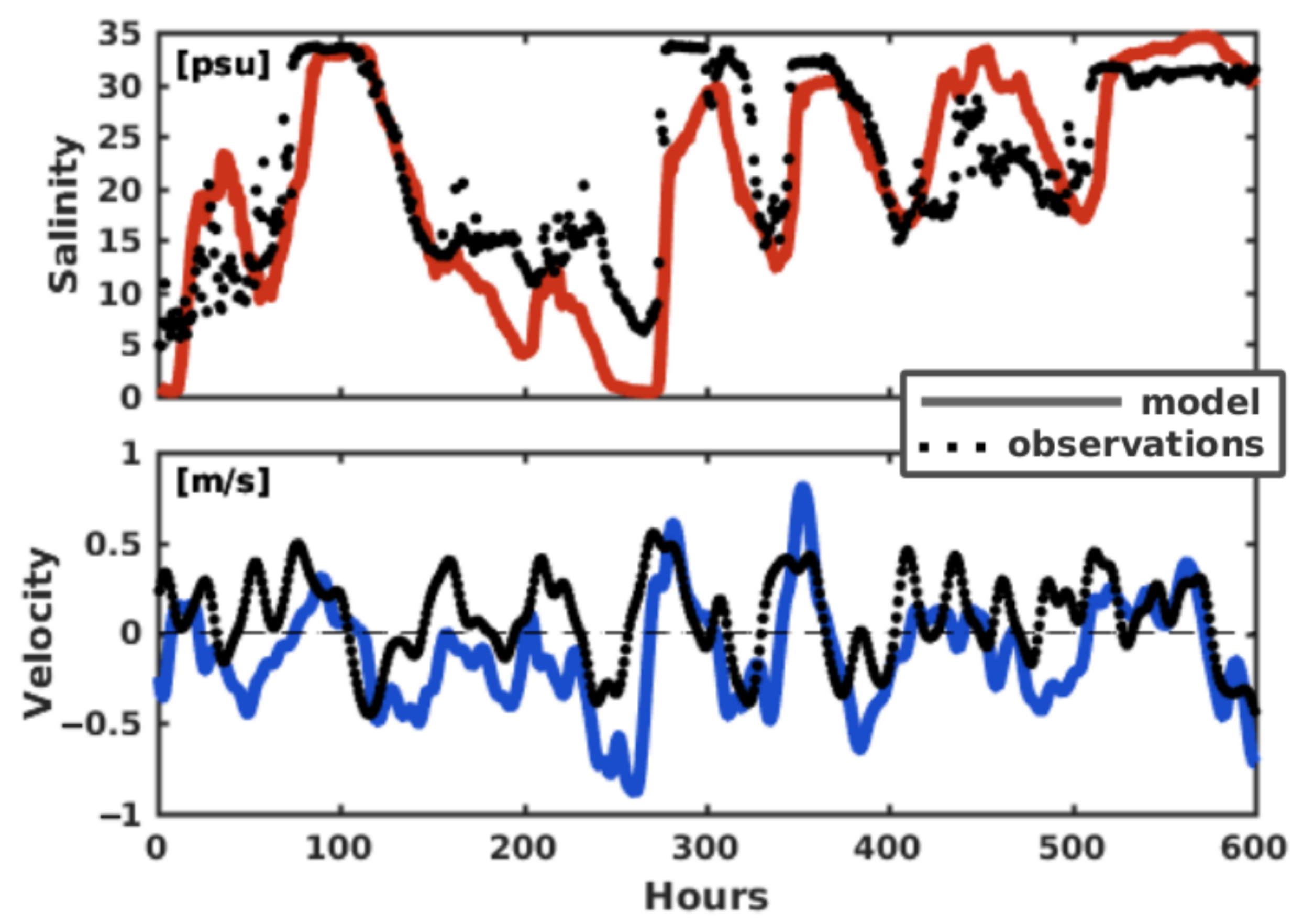
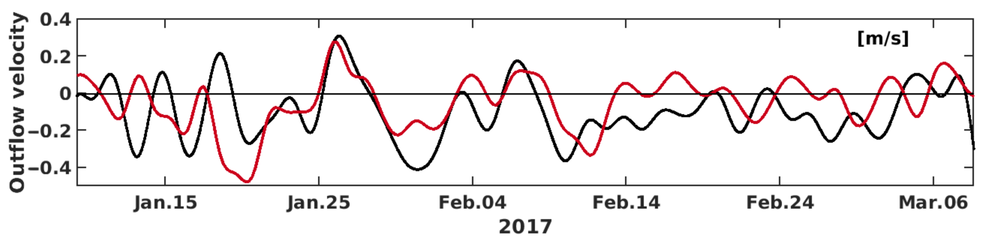
2.5. Validation of the Hydrodynamic Model

Results from the hydrodynamic model were validated using observations of current and salinity at the interior of the channel and observations at the inner shelf, nearby to the jetties.Water level along the Patos Lagoon is also used to callibrate the cycle of ebb and flood in the domain, which drive the plume’s outflow. The performance of the model was measured using the mean squared error (MSE) and bias [49].

Current and salinity observations were obtained by an acoustic Doppler current profiler (ADCP) fixed at the Pilot Station (Figure 1, red square in frame b) in the estuary channel between January and February of 2011. Figure 4 shows the time series of observations (black dotted lines) and the model (colored lines) for a period of 600 h. The model correctly reproduced the cycles of ebbing (flooding), as shown by lower (higher) values of salinity and negative (positive) values of velocity. For the salinity, the performance as measured was MSE = 5.97 psu and bias = −1.47 psu, while for the velocity, it was MSE = 0.32 ms ${}^{-1}$ and bias = −0.20 ms ${}^{-1}$. Overall, the model underestimated the salinity and velocity, which is related to the absence of rain and the discharges of smaller rivers.

Observations of outflow velocities were registered at the inner shelf by the oceanographic buoy RS-5 (Figure 1, pink square in frame b) installed by the “Sistema de Monitoramento da Costa Brasileira” (SiMCosta—www.simcosta.furg.b, accessed on 6 April 2018). These observations were compared with the model results for 58 days along January and March of 2017 and presented in Figure 5. Simulated and observed velocities showed better agreement during ebb conditions, with MSE = 0.15 ms ${}^{-1}$ and bias = 0.07 ms ${}^{-1}$. Discrepancies between observed and modeled velocities are related to the strong turbulence generated by the plume outflow, mainly because the period is marked by a nearly slack water condition, with weak velocities for ebb and flood. This particular condition can result in higher inaccuracy over the velocity field, since the model do not reproduce the influence of the wave field (captured by the observed data), and hence the wave-current interaction [35,50].

The validation of the simulated drifters is absent because of lacking of Lagrangian observations. The reliability of the drifter module can be acquired by previous works involving derivations of the Lagrangian module used in this work: used to infer patterns of transport in a choked lagoon in the work of [51], which is well correlated with sediment distributions [52], and the reproduction of trajectories of oil spills occurred in a coastal beach conducted by [36].

Observations of water level at the stations of Ipanema, Arambaré and São Lourenço for 2012 were acquired from ANA and showed in Figure 6. The comparison between the model and observations was made by removing the means of both time series. Figure 6 shows the level anomaly as observed (black dots) and modeled (blue line) for the three stations. The model shows good agreement with the observed variability at all stations, which is related to the riverine discharge and wind setup on the lagoon. For the Ipanema station, MSE = $15.2$ cm and bias = $9.6$ cm, at the Arambaré station, MSE = $17.1$ cm and bias = $11.20$ cm, and at the São Lourenço station, MSE = 18.7 cm and bias = $13.3$ cm. The main limitation of your model is the absence of hydrologic parametrization and precipitation, which can contribute for some inaccurate at the lower sector of the lagoon.

3. Results and Discussion

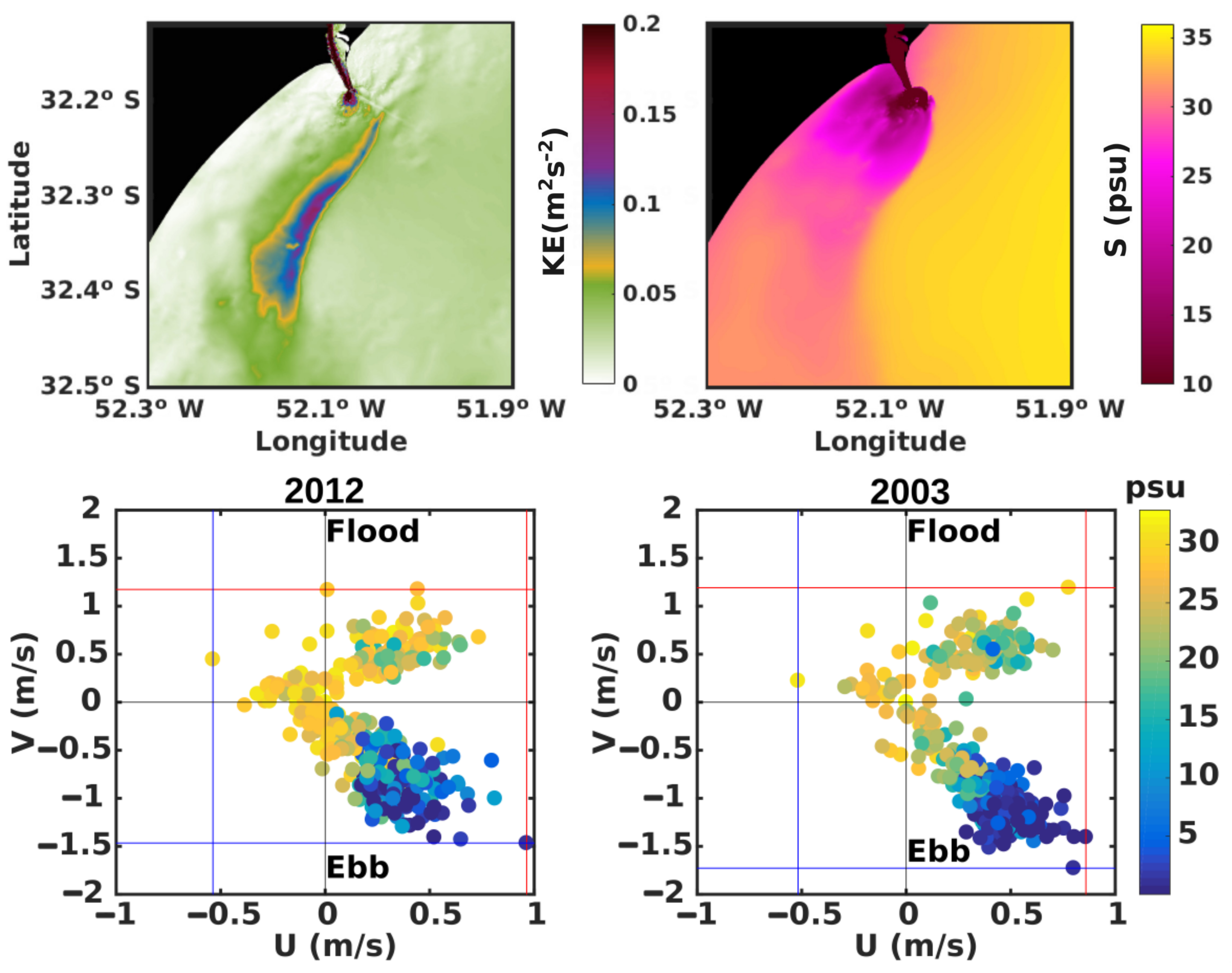
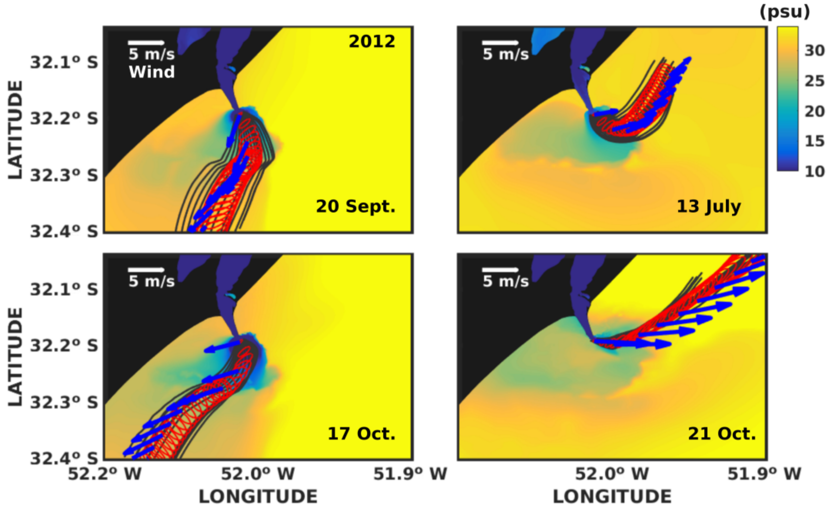
3.1. Plume Circulation Pattern

Before discussing the spreading of the drifters, we characterize the general circulation pattern and dynamics of the hindcast simulations. The Patos Lagoon coastal plume simulations exhibit a high variability over the inner shelf, associated with the velocity and salinity field, which is marked by an abrupt change at the plume front.

The plume field variability is driven by the local and non-local wind influences acting on the sea and on the lagoon water level. The upper panel of Figure 7 presents the results for salinity and kinetic energy ( $KE=(U^2+V^2)/2$) fields for 20 February 2003. The width of the low salinity (<26 psu) water of the plume could reach distances from the inlet of approximately 20 km. The dominant time scale of the outflow of freshwater is 8 days, primarily due to a cold front passage [53]. The observed southward propagation of the plume is due to northeast winds (upwelling favorable) with intensities >8 ms ${}^{-1}$. Along the plume’s front, a band of higher KE values (>0.1 m ${}^2$ s ${}^{-2}$) is characterized by convergence of currents enhanced by baroclinic gradients. In addition to the large variability of the coastal plume, in terms of area and southward or northward propagation, these velocity features along the plume front are maintained.

The riverine discharge in the interior of the lagoon is responsible for the plume outflow modulation. Increases in discharge are followed by subsequent enhancement of the ebb flows through the inlet. The lower panel of Figure 7 shows results for the 2012 and 2003 simulations regarding the distribution of mean zonal and meridional velocities at the mouth of the jetties, and the corresponding salinity values are superposed to the color scale. The ebbing events are distinguished by negative values of meridional velocities V and low values of salinity.

According to [54], an increment in outward flow associated with riverine discharge occurs due to the increase in pressure gradient at the estuarine zone. This is verified by the velocity distributions for both years. For 2003, ebb currents are more frequent and more intense as a function of the relative higher discharge for that year.

These contrasts are associated with the riverine discharge differences imposed for the two years. Ref. [55] report that the long-term variability of the freshwater discharge is responsible for 50% of the variability of the levels at the estuarine portion of the Patos Lagoon. In addition to external sources of variability, freshwater discharge is the major cause of the differences in plume outflow velocities between the results of the 2003 and 2012 simulations. Thus, the differences for the thickness and width of the plume resulting from these discharge influences are discussed in the followed subsection.

3.2. Dynamical Classification

All the scale parameters present differences related to the amount of riverine discharge for the 2003 and 2012 simulations. The discharge influence over the plume is shown through the extent of the low salinity signature of the Patos Lagoon Coastal Plume. Here, we discuss the discharge role over the coastal plume, comparing results sampled from the red dot marked on frame c of Figure 1 from both simulations.

Hovmöller diagrams of the vertical salinity for both simulations are shown in Figure 8. The experiment for 2012 presents events with stronger stratification by July, corresponding to the increase in the riverine discharge (Figure 2). The averaged plume thickness (the 26 psu isohaline, white line in the diagram) are 4 m, and the plume is the majority surface advected. In contrast, 2003 shows lower values of salinity for longer periods, with short events of stratification. The averaged plume thickness is 8 m, and events in which the 26 psu isohaline is attached to the bottom are more frequent than for the simulation of 2012. Using a potential energy analysis, ref. [6] demonstrate that the stratification at the inlet is controlled by alongshore and cross-shore advection processes and by alongshore straining processes. Hence, contrasts between the two simulations are explained by the gravitational contribution of the riverine discharge to the seaward flow.

The cycles of stratification are controlled by the alternation between ebbing and flooding entwined to its favorable winds. Nevertheless, the higher plume thickness for the 2003 simulation is due to the superior average riverine discharge for that year. Previous works also reported a significant reduction in the salinity adjacent to the inlet zone for high riverine discharge events [56]. These occur due to the combination of riverine discharge with wind setup at the lagoon’s interior, which strengthens plume outflow [28]. Previous studies showed that a discharge >2000 m ${}^3$ s ${}^{-1}$ is sufficiently high to overcome the pressure gradient induced by the winds that promote flooding events [54], which is responsible for the prevalence of lower salinity for the 2003 simulation (see Figure 2, for the prevalence of north quadrant winds).

The scale parameters were applied to each experiment (

Table 1. Scale parameters of the plume for both simulations.

Scale Parameters	2003	2012
$R_D$ (km)	11.42	10.39
$K_b$	0.10	0.26
R	0.85	1.28
$E_k$	0.20	0.81
$Fr$	0.85	1.28
$K_m$	0.06	0.06
$R{e}_p$	4.22	1.58
$Ri$	1.34	0.71

). All the parameters presented typical values for a small scale plume strongly controlled by wind forcing. The $R_D$ for both experiments are on the order of 10 km. The $K_b$ present values ranging from 0.10 to 0.26, indicating that the width of the plume is smaller than $R_D$ for both cases. Values for R are closer to unity, showing a equal balance between the plume jet flow and the influence of the rotation. For $K_m$, differences between the two cases are negligible, while $K_m$ = 0.06 implies that the size of the inlet mouth is favorable to the formation of a bulge. These scale parameters show that the plume is moderately governed by inertial and rotational processes.

Due to large oscillation of the flow velocity in addition to the density field, values for $Fr$ show that the stratification and inertia play a similar role on the plume flow. The $E_k$ indicate that for the high discharge regime, rotations are more important, while for the low discharge regime, the rotational processes are balanced by frictional processes. Frictional processes are also related to the wind and bottom stress, as evaluated by the work of [54]. The $R{e}_p$ for the two simulations are >1, suggesting that inertia governs the flow, and for the high discharge regime, inertial processes are enhanced. The average value of the $Ri$ shows that at high discharge, the mixture are relatively superior to the stratification processes.

The values of the scale parameters are compatible with the range observed for diverse coastal plumes, which have some similarities with the Patos Lagoon coastal plume [7]. Differences between the high and low discharge periods are comparable to the results of [57] for the downwelling and upwelling events of the plumes of the Minho and Douro rivers (Italy). In summary, the plume is characterized as being a small-scale surface advected plume, where the riverine discharge significantly alters the dynamics of the flow.

Time series of $Ri$ for each simulation are shown in the lower panel of Figure 8. The variability of the $Ri$ for both experiments are correlated with the cycles of stratification. This variability occurs due to changes in vertical velocity shear and density fields. Events with $Ri$ < 0.25 are more frequent in the simulation of 2003 than in 2012, meaning that during the low discharge regime, the values of $Ri$ represent that the outflow cannot overturn the stratification. At periods during which the riverine discharge is sufficiently high (up to 2000 m ${}^3$ s ${}^{-1}$, Figure 2), the plume outflow nullifies the stratification, as observed by the $Ri$ values in 2003.

Similar periodicities for the $Ri$ through the buoyancy flux at the continental shelf are documented for other regions of riverine influence [48,58]. Differences highlighted by the results presented in Figure 8 summarize the effect that the amount of riverine discharge has overthe plume structure, whichis reflected over the width and thickness of the plume bulge due to gravitational adjustment [59].

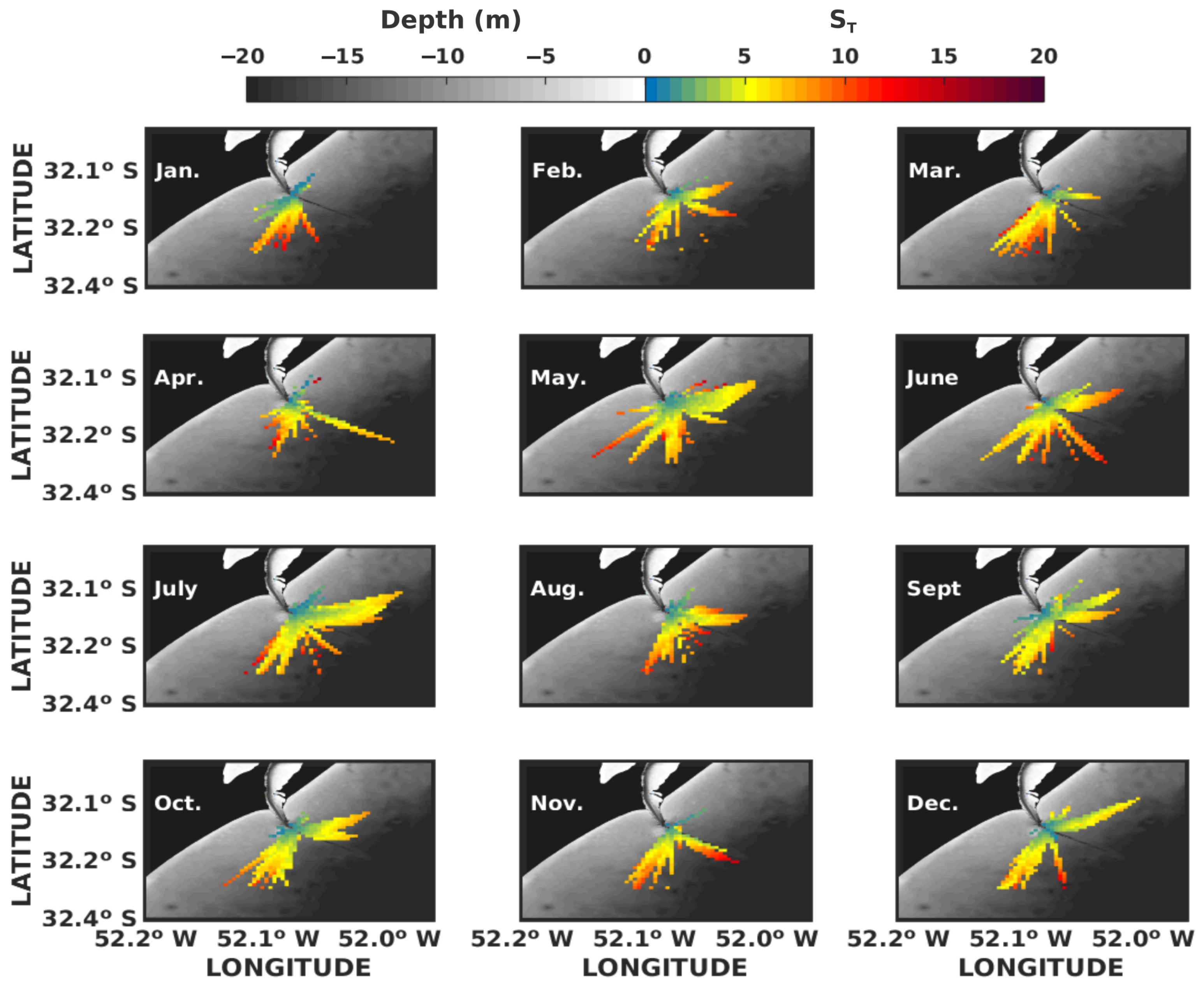
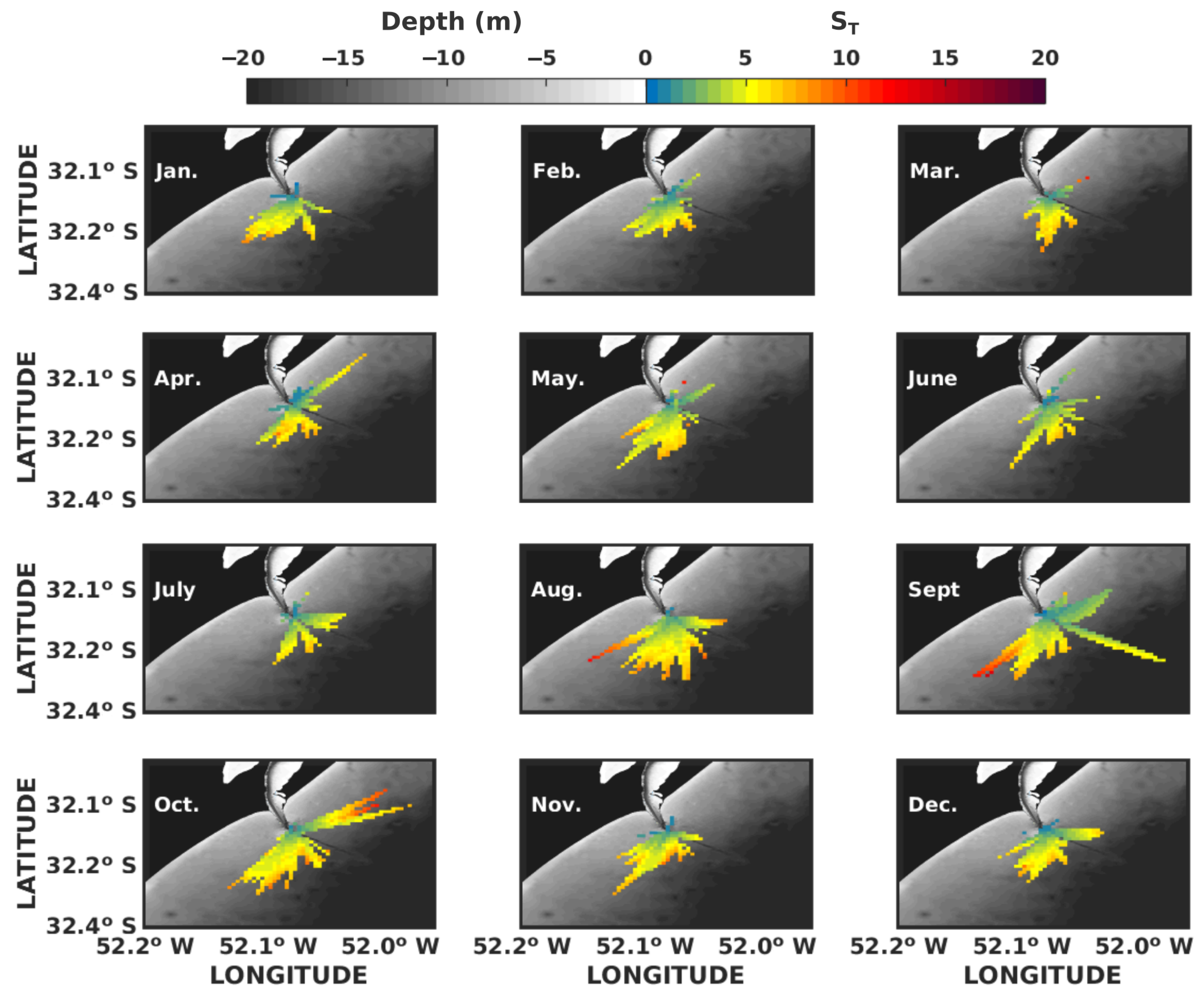
3.3. Trajectories of the Drifters

Here, we present details of a selection of drifter trajectories in order to discuss the ways that the plume and wind affect the drifters’ spreading. Figure 9 shows four episodes of drifter releases during 2012 for a period of 10 h. The $S_x$ and $S_y$ along the r are superposed on the individual trajectories of drifters in relation to the axes of ellipsoids.

Figure 9 shows four events with varying forcing dynamics leading to contrasting plume outflows. The background scale presents the salinity field, the blue vectors represent wind velocity, and the solid lines represent the drifters’ trajectories. The red ellipsoids represent the spreading of the drifters, where the major and minor axes are centered along the center of mass of the drifters. For instance, the events of 20 September and 17 October are associated with a typical feature of north quadrant winds associated with a strong outflow southwards. In opposition, events of 13 July and 21 October rely on south quadrant winds, which induce outflows northward, before suppressing the plume due to the flood event induced by those downwelling winds.

Except for 21 October, the spread patterns of the drifters are subjected to an abrupt change outside of the plume (marked by lower salinity). Events on 20 September and 17 October presented similar wind intensities (5.0 ms ${}^{-1}$), although with slight differences in direction. On 20 September, a north wind is predominant which favors the outflow, and on 17 October, the northeast wind enhances the bending of the plume towards the coast. For these cases when the drifters leave the field of the plume, an abrupt change occurs in the direction of motion of the cluster and the spreading of the drifters. This change is due to the convergence of horizontal velocities, which occurs along the plume front associated with the density gradients. For both cases, the increase in along shore spreading ( $S_y$) is enhanced at the plume’s field. Outside of the plume, the drifters are advected by coastal currents, and the values for $S_x$ and $S_y$ remain approximately constant.

The plumes on 13 July and 21 October are events related to the onset of southwest winds. Drifters on 13 July are subjected to alongshore spreading at the plume field, while at the plume front, the cross-shore spreading increases and remains approximately constant when advected by the coastal currents. On 21 October, an intense southwest wind (8 ms ${}^{-1}$) enhances the coastal currents, and the drifters are strongly advected northward. The spreading in the cross-shore axis is suppressed by the alongshore displacement of the drifters. Hence, the effects of the plume field over the drifters’ alongshore spreading are superposed on strong currents. Ref. [60] also report coherent circulation structures related to the jetties, which contributes to the pattern of trajectories of the simulated drifters.

These selected events demonstrate the nearfield influence of the plume over the trajectories of the drifters. The increasing of buoyancy flux rate promotes the extended plume field [61], where its extension is responsible for the initial alongshore pathways followed by the drifters.The wind is responsible by the outflow and drive coastal mixing and stirring mechanisms [21], which influence the transport of drifters. Coastal currents driven by the wind also suppress the transport alongshore. Thus, the magnitude of the riverine discharge represent a additional factor over the trajectories of the drifters.

3.4. Drifter’s Spreading

Both simulations have similar wind conditions, hence the major contrasts between these results are due to differences in the total riverine discharge being used as boundary conditions. The contrasts are highlighted by the intensity of the advection of the drifters, which result in differences in the total spreading along the cross/alongshore axes.

The total spreading $S_T$ are presented in Figure 10 and Figure 11, which capture differences of magnitude for $S_x$ and $S_y$ (not showed). The extent of the binned grid shows how far the center of mass of the drifters is transported away from the inlet mouth after 5 h from the release. After pulses of higher discharge the drifters are advected for longer distances in the same time interval, and the wind play a significant role over the direction of the advection to southward or northward. Months that are subjected to peaks of riverine discharge (March and from May to October) presents higher values of $S_T$. The results shows that in the simulation of 2003 the drifters reached longer distances and exhibit a more intense spreading when compared with 2012.

The two simulations shows the impact of the riverine discharge over the fields of $S_T$. A higher riverine discharge enhances the plume outflow, which significantly modifies the plume structure and the characteristics of the flow (see Figure 8). A higher outflow promotes an extension of the plume field and an increase in its radial spreading [14], since that increase in the buoyancy flux also increases the pressure gradient, which favors the alongshore spreading [62]. The enhancement of the spreading of the plume caused by higher discharge besides wind variability, indicate that riverine outflow can alter the penetration of these coastal plume further in the inner shelf.

Ref. [15] report that drifter data for four coastal plumes of the Southern California Bight alongshore currents are responsible for restricting the cross-shore spreading. The development of strong coastal currents adjacent to our study area showed a similar effect. However, the results from the simulation of 2003 shows that the increase in the plume outflow favors cross-shore spreading. The bathymetry of the entrance channel also favor the outflow along the cross-shore direction. This enhance the capacity of the plume to overcome the coastal currents and to spread in the cross-shore direction [63].

A high discharge plume is responsible for a spreading uncorrelated with the wind direction, but the outflow of Patos Lagoon Plume is mainly controlled by meteorological tides. Hence, the higher values of $S_T$ for 2003, results from the higher riverine discharge added to outflow caused by the wind stress. These addition to the outflow enhanced the $S_T$ from a average of 10 to 15 (normalized width) at the nearfield, respectively, to the cases of 2012 and 2003. Ref. [21] shows the importance of the wind stress to drive offshore transport for a small plume, which agree with our results for events of meteorological ebbing. Furthermore, moderate wind still can modify the direction from the middle-field and far-field due mixing and dilution with the water of the inner shelf [64]. Thus, events of transition from high to moderate discharge become more sensible to be driven by wind stress.

Comparison with the coastal plumes of the Merrimack River (USA) and New River (USA) shows similarities. The plume of Merrimack River also have ratios of alongshore superior to the cross-shore spreading, as estimated by [42]. Using observed drifters in New River’s plume, ref. [65] shows that higher spreading occurs when the drifters reached deeper areas in the coastal zone, likewise our results. These similarities indicates when the outflow of the Patos Lagoon is enhanced, the plume extend the region of spreading over the inner shelf. Thus, our results can be used as a proxy to describe how the riverine discharge changes the pattern of transport of material delivered by the plume along the adjacent areas, which is strongly dependent of the value of $S_T$ [13,66].

In summary, the riverine discharge showed a major role to extend the influence of the plume over the inner continental shelf. Since the variability of the outflow occurs due the wind stress, but is the amount of riverine discharge which is capable to enhance the outflow at the inlet, and therefore increase the spreading of the plume.

4. Conclusions

Under similar wind conditions, the major effects of the differences in discharge regime were over the salinity field and velocities adjacent to the inlet mouth. Vertical distribution of salinity presented values lower in 2003 than in 2012; the simulation for 2003 also showed fewer periods of stratification. Scale parameters measured the distinctions between both simulations, highlighted by contrasts in plume width, plume thickness and by vertical velocity shear. The scale parameters highlight that the Patos Lagoon Coastal Plume are strongly affected by the wind, but for higher discharges regimes, the inertial processes are enhanced.

The drifters showed a more intense advection during high discharge periods during 2003 when compared to the low discharge period of 2012. The total spreading calculated also presented enhanced values in the simulation of 2003. The riverine discharge showed an important role over the capacity of the Patos Lagoon Coastal plume to spread radially over the inner shelf. For a small outflow, the results of this work highlight the variability of the spreading of this coastal plume.

Since the spreading of the coastal plume is associated with the strength of its mixing with the surrounding environment, this study provides insight into how the Patos Lagoon plume has the potential to disperse and deliver terrigenous material on the coastal zone and inner shelf depending on the amount of discharge which enhance the outflow of this coastal plume.

References

1. Trenberth, K.E.; Smith, L.; Qian, T.; Dai, A.; Fasullo, J. Estimates of the global water budget and its annual cycle using observational and model data. J. Hydrometeorol. 2007, 8, 758–769. [Google Scholar] [CrossRef]
2. Sharples, J.; Middelburg, J.J.; Fennel, K.; Jickells, T.D. What proportion of riverine nutrients reaches the open ocean? In Global Biogeochemical Cycles; Wiley: New York, NY, USA, 2016. [Google Scholar]
3. Vizy, E.K.; Cook, K.H. Influence of the Amazon/Orinoco Plume on the summertime Atlantic climate. J. Geophys. Res. Atmos. 2010, 115, D21112. [Google Scholar] [CrossRef]
4. Milliman, J.D.; Syvitski, J.P. Geomorphic/tectonic control of sediment discharge to the ocean: The importance of small mountainous rivers. J. Geol. 1992, 100, 525–544. [Google Scholar] [CrossRef]
5. Wheatcroft, R.A.; Hatten, J.A.; Pasternack, G.B.; Warrick, J.A.; Goni, M.A. The role of effective discharge in the ocean delivery of particulate organic carbon by small, mountainous river systems. Limnol. Oceanogr. 2010, 55, 161–171. [Google Scholar] [CrossRef] [Green Version]
6. Marques, W.C.; Fernandes, E.H.; Moller, O.O. Straining and advection contributions to the mixing process of the Patos Lagoon coastal plume, Brazil. J. Geophys. Res. Ocean. 2010, 115, 1–23. [Google Scholar] [CrossRef] [Green Version]
7. Garvine, R.W. A dynamical system for classifying buoyant coastal discharges. Cont. Shelf Res. 1995, 15, 1585–1596. [Google Scholar] [CrossRef]
8. Horner-Devine, A.R.; Hetland, R.D.; MacDonald, D.G. Mixing and transport in coastal river plumes. Annu. Rev. Fluid Mech. 2015, 47, 569–594. [Google Scholar] [CrossRef]
9. O’Donnell, J.; Ackleson, S.G.; Levine, E.R. On the spatial scales of a river plume. J. Geophys. Res. Ocean. 2008, 113, 1–3. [Google Scholar] [CrossRef] [Green Version]
10. Marques, W.; Fernandes, E.; Monteiro, I.; Möller, O. Numerical modeling of the Patos Lagoon coastal plume, Brazil. Cont. Shelf Res. 2009, 29, 556–571. [Google Scholar] [CrossRef]
11. Hetland, R.D. Relating river plume structure to vertical mixing. J. Phys. Oceanogr. 2005, 35, 1667–1688. [Google Scholar] [CrossRef]
12. Yankovsky, A.E.; Chapman, D.C. A simple theory for the fate of buoyant coastal discharges. J. Phys. Oceanogr. 1997, 27, 1386–1401. [Google Scholar] [CrossRef] [Green Version]
13. Yuan, Y.; Horner-Devine, A.R. Laboratory investigation of the impact of lateral spreading on buoyancy flux in a river plume. J. Phys. Oceanogr. 2013, 43, 2588–2610. [Google Scholar] [CrossRef]
14. Jurisa, J.T.; Nash, J.D.; Moum, J.N.; Kilcher, L.F. Controls on Turbulent Mixing in a Strongly Stratified and Sheared Tidal River Plume. J. Phys. Oceanogr. 2016, 46, 2373–2388. [Google Scholar] [CrossRef]
15. Warrick, J.A.; DiGiacomo, P.M.; Weisberg, S.B.; Nezlin, N.P.; Mengel, M.; Jones, B.H.; Ohlmann, J.C.; Washburn, L.; Terrill, E.J.; Farnsworth, K.L. River plume patterns and dynamics within the Southern California Bight. Cont. Shelf Res. 2007, 27, 2427–2448. [Google Scholar] [CrossRef]
16. Bao, H.; Lee, T.Y.; Huang, J.C.; Feng, X.; Dai, M.; Kao, S.J. Importance of Oceanian small mountainous rivers (SMRs) in global land-to-ocean output of lignin and modern biospheric carbon. Sci. Rep. 2015, 5, 16217. [Google Scholar] [CrossRef] [PubMed] [Green Version]
17. Osadchiev, A.; Korotenko, K.; Zavialov, P.; Chiang, W.S.; Liu, C.C. Transport and bottom accumulation of fine river sediments under typhoon conditions and associated submarine landslides: Case study of the Peinan River, Taiwan. Nat. Hazards Earth Syst. Sci. 2016, 16, 41–54. [Google Scholar] [CrossRef]
18. Ostrander, C.E.; McManus, M.A.; DeCarlo, E.H.; Mackenzie, F.T. Temporal and spatial variability of freshwater plumes in a semienclosed estuarine-bay system. Estuaries Coasts 2008, 31, 192. [Google Scholar] [CrossRef]
19. Pimenta, F.M.; Kirwan, A., Jr. The response of large outflows to wind forcing. Cont. Shelf Res. 2014, 89, 24–37. [Google Scholar] [CrossRef]
20. Suanda, S.H.; Kumar, N.; Miller, A.J.; Di Lorenzo, E.; Haas, K.; Cai, D.; Edwards, C.A.; Washburn, L.; Fewings, M.R.; Torres, R.; et al. Wind relaxation and a coastal buoyant plume north of Pt. Conception, CA: Observations, simulations, and scalings. J. Geophys. Res. Ocean. 2016, 121, 7455–7475. [Google Scholar] [CrossRef]
21. Zhao, J.; Gong, W.; Shen, J. The effect of wind on the dispersal of a tropical small river plume. Front. Earth Sci. 2018, 12, 170–190. [Google Scholar] [CrossRef]
22. Huang, W.; Li, C.; White, J.R.; Bargu, S.; Milan, B.; Bentley, S. Numerical experiments on variation of freshwater plume and leakage effect from Mississippi River Diversion in the Lake Pontchartrain Estuary. J. Geophys. Res. Ocean. 2020, 125, e2019JC015282. [Google Scholar] [CrossRef]
23. Orton, P.M.; Jay, D.A. Observations at the tidal plume front of a high-volume river outflow. Geophys. Res. Lett. 2005, 32, 1–4. [Google Scholar] [CrossRef] [Green Version]
24. Kilcher, L.F.; Nash, J.D.; Moum, J.N. The role of turbulence stress divergence in decelerating a river plume. J. Geophys. Res. Ocean. 2012, 117, 1–15. [Google Scholar] [CrossRef] [Green Version]
25. Rong, Z.; Hetland, R.D.; Zhang, W.; Zhang, X. Current–wave interaction in the Mississippi–Atchafalaya river plume on the Texas–Louisiana shelf. Ocean. Model. 2014, 84, 67–83. [Google Scholar] [CrossRef] [Green Version]
26. Zavialov, P.; Möller, O.; Campos, E. First direct measurements of currents on the continental shelf of southern Brazil. Cont. Shelf Res. 2002, 22, 1975–1986. [Google Scholar] [CrossRef]
27. Burrage, D.; Wesson, J.; Martinez, C.; Pérez, T.; Möller, O.; Piola, A. Patos Lagoon outflow within the Río de la Plata plume using an airborne salinity mapper: Observing an embedded plume. Cont. Shelf Res. 2008, 28, 1625–1638. [Google Scholar] [CrossRef]
28. Möller, O.O.; Castaing, P.; Salomon, J.C.; Lazure, P. The influence of local and non-local forcing effects on the subtidal circulation of Patos Lagoon. Estuaries Coasts 2001, 24, 297–311. [Google Scholar] [CrossRef]
29. Möller, O.O.; Castaing, P.; Fernandes, E.H.L.; Lazure, P. Tidal frequency dynamics of a southern Brazil coastal lagoon: Choking and short period forced oscillations. Estuaries Coasts 2007, 30, 311–320. [Google Scholar] [CrossRef]
30. Zavialov, P.; Kostianoy, A.; Möller, O. SAFARI cruise: Mapping river discharge effects on Southern Brazilian shelf. Geophys. Res. Lett. 2003, 30, 1–4. [Google Scholar] [CrossRef]
31. Zavialov, P.; Pelevin, V.; Belyaev, N.; Izhitskiy, A.; Konovalov, B.; Krementskiy, V.; Goncharenko, I.; Osadchiev, A.; Soloviev, D.; Garcia, C.; et al. High resolution LiDAR measurements reveal fine internal structure and variability of sediment-carrying coastal plume. Estuar. Coast. Shelf Sci. 2018, 205, 40–45. [Google Scholar] [CrossRef]
32. Fernandes, E.; Dyer, K.; Moller, O.; Niencheski, L. The Patos Lagoon hydrodynamics during an El Niño event (1998). Cont. Shelf Res. 2002, 22, 1699–1713. [Google Scholar] [CrossRef]
33. Fernandes, E.H.L.; Dyer, K.R.; Moller, O.O. Spatial gradients in the flow of southern Patos Lagoon. J. Coast. Res. 2005, 20, 759–769. [Google Scholar] [CrossRef]
34. Marques, W.C.; Fernandes, E.H.; Moraes, B.C.; Möller, O.O.; Malcherek, A. Dynamics of the Patos Lagoon coastal plume and its contribution to the deposition pattern of the southern Brazilian inner shelf. J. Geophys. Res. Ocean. 2010, 115, 1–22. [Google Scholar] [CrossRef]
35. Hervouet, J.M. Free Surface Flows: Modelling with Finite Element Methods; John Wiley & Sons: Hoboken, NJ, USA, 2007. [Google Scholar]
36. Marques, W.; Stringari, C.; Kirinus, E.; Möller, O., Jr.; Toldo, E., Jr.; Andrade, M. Numerical modeling of the Tramandaí beach oil spill, Brazil—Case study for January 2012 event. Appl. Ocean. Res. 2017, 65, 178–191. [Google Scholar] [CrossRef]
37. Cucco, A.; Umgiesser, G. Modeling the Venice Lagoon residence time. Ecol. Model. 2006, 193, 34–51. [Google Scholar] [CrossRef]
38. Chassignet, E.P.; Hurlburt, H.E.; Smedstad, O.M.; Halliwell, G.R.; Hogan, P.J.; Wallcraft, A.J.; Baraille, R.; Bleck, R. The HYCOM (hybrid coordinate ocean model) data assimilative system. J. Mar. Syst. 2007, 65, 60–83. [Google Scholar] [CrossRef]
39. Egbert, G.D.; Erofeeva, S.Y. Efficient inverse modeling of barotropic ocean tides. J. Atmos. Ocean. Technol. 2002, 19, 183–204. [Google Scholar] [CrossRef] [Green Version]
40. Pham, C.T.; Joly, A. Telemac Modelling System: Telemac-3D Software—Operating Manual; Technical Report; EDF: Chateau, France, 2016. [Google Scholar]
41. Simmons, A.; Uppala, S.; Dee, D.; Kobayashi, S. ERA-Interim: New ECMWF reanalysis products from 1989 onwards. Ecmwf Newsl. 2007, 110, 25–35. [Google Scholar]
42. Chen, F.; MacDonald, D.G.; Hetland, R.D. Lateral spreading of a near-field river plume: Observations and numerical simulations. J. Geophys. Res. Ocean. 2009, 114, 1–12. [Google Scholar] [CrossRef]
43. Fontoura, J.A.; Almeida, L.E.; Calliari, L.J.; Cavalcanti, A.M.; Möller, O., Jr.; Romeu, M.A.R.; Christófaro, B.R. Coastal Hydrodynamics and Longshore Transport of Sand on Cassino Beach and on Mar Grosso Beach, Southern Brazil. J. Coast. Res. 2012, 29, 855–869. [Google Scholar] [CrossRef]
44. Bennett, A. Relative dispersion: Local and nonlocal dynamics. J. Atmos. Sci. 1984, 41, 1881–1886. [Google Scholar] [CrossRef] [Green Version]
45. Cushman-Roisin, B.; Beckers, J.M. Introduction to Geophysical Fluid Dynamics: Physical and Numerical Aspects; Academic Press: Cambridge, MA, USA, 2011; Volume 101. [Google Scholar]
46. Tilburg, C.E.; Gill, S.M.; Zeeman, S.I.; Carlson, A.E.; Arienti, T.W.; Eickhorst, J.A.; Yund, P.O. Characteristics of a shallow river plume: Observations from the Saco River Coastal Observing System. Estuaries Coasts 2011, 34, 785–799. [Google Scholar] [CrossRef]
47. Chao, S.Y. Wind-driven motion of estuarine plumes. J. Phys. Oceanogr. 1988, 18, 1144–1166. [Google Scholar] [CrossRef] [Green Version]
48. Sanders, T.M.; Garvine, R.W. Fresh water delivery to the continental shelf and subsequent mixing: An observational study. J. Geophys. Res. Ocean. 2001, 106, 27087–27101. [Google Scholar] [CrossRef]
49. Thomson, R.E.; Emery, W.J. Data Analysis Methods in Physical Oceanography; Newnes: London, UK, 2014. [Google Scholar]
50. Qu, L.; Hetland, R.D. Temporal resolution of wind forcing required for river plume simulations. J. Geophys. Res. Ocean. 2019, 124, 1459–1473. [Google Scholar] [CrossRef]
51. Silva, D.V.D.; Oleinik, P.H.; Costi, J.; de Paula Kirinus, E.; Marques, W.C. Residence time patterns of Mirim Lagoon (Brazil) derived from two-dimensional hydrodynamic simulations. Environ. Earth Sci. 2019, 78, 163. [Google Scholar] [CrossRef]
52. Vieira, H.M.; Weschenfelder, J.; Fernandes, E.H.; Oliveira, H.A.; Möller, O.O.; García-Rodríguez, F. Links between surface sediment composition, morphometry and hydrodynamics in a large shallow coastal lagoon. Sediment. Geol. 2020, 398, 105591. [Google Scholar] [CrossRef]
53. Marques, W.C.; Monteiro, I.O.; Möller, O.O. The Exchange Processes in the Patos Lagoon Estuarine Channel, Brazil. Int. J. Geosci. 2011, 2, 248. [Google Scholar] [CrossRef] [Green Version]
54. Castelao, R.M.; Moller, O.O., Jr. A modeling study of Patos Lagoon (Brazil) flow response to idealized wind and river discharge: Dynamical analysis. Braz. J. Oceanogr. 2006, 54, 1–17. [Google Scholar] [CrossRef]
55. Barros, G.; Marques, W. Long-Term Temporal Variability of the Freshwater Discharge and Water Levels at Patos Lagoon, Rio Grande do Sul, Brazil. Int. J. Geophys. 2012, 2012, 459497. [Google Scholar] [CrossRef]
56. Barros, G.P.; Marques, W.C.; Kirinus, E.D.P. Influence of the freshwater discharge on the hydrodynamics of Patos Lagoon, Brazil. Int. J. Geosci. 2014, 2014, 925–942. [Google Scholar] [CrossRef] [Green Version]
57. Mendes, R.; Sousa, M.C.; Gómez-Gesteira, M.; Dias, J.M.; de Castro, M. New insights into the Western Iberian Buoyant Plume: Interaction between the Douro and Minho River plumes under winter conditions. Prog. Oceanogr. 2016, 141, 30–43. [Google Scholar] [CrossRef]
58. Lentz, S.J.; Largier, J. The influence of wind forcing on the Chesapeake Bay buoyant coastal current. J. Phys. Oceanogr. 2006, 36, 1305–1316. [Google Scholar] [CrossRef]
59. Yankovsky, A.E.; Hickey, B.M.; Münchow, A.K. Impact of variable inflow on the dynamics of a coastal buoyant plume. J. Geophys. Res. Ocean. 2001, 106, 19809–19824. [Google Scholar] [CrossRef] [Green Version]
60. Hodapp, M.J.; Kirinus, E.d.P.; Marques, W.C.; Oleinik, P.H.; Moller, O.O. Investigation of persistent coherent structures along the Southern Brazilian Shelf. Braz. J. Oceanogr. 2018, 66, 199–209. [Google Scholar] [CrossRef] [Green Version]
61. Warrick, J.A.; Stevens, A.W. A buoyant plume adjacent to a headland—Observations of the Elwha River plume. Cont. Shelf Res. 2011, 31, 85–97. [Google Scholar] [CrossRef]
62. McCabe, R.M.; MacCready, P.; Hickey, B.M. Ebb-Tide Dynamics and Spreading of a Large River Plume*. J. Phys. Oceanogr. 2009, 39, 2839–2856. [Google Scholar] [CrossRef]
63. Feddersen, F.; Olabarrieta, M.; Guza, R.; Winters, D.; Raubenheimer, B.; Elgar, S. Observations and modeling of a tidal inlet dye tracer plume. J. Geophys. Res. Ocean. 2016, 121, 7819–7844. [Google Scholar] [CrossRef]
64. Osadchiev, A.; Sedakov, R.; Barymova, A. Response of a small river plume on wind forcing. Front. Mar. Sci. 2021, 8, 1–9. [Google Scholar] [CrossRef]
65. Spydell, M.S.; Feddersen, F.; Olabarrieta, M.; Chen, J.; Guza, R.; Raubenheimer, B.; Elgar, S. Observed and modeled drifters at a tidal inlet. J. Geophys. Res. Ocean. 2015, 120, 4825–4844. [Google Scholar] [CrossRef]
66. Blanken, H.; Hannah, C.; Klymak, J.M.; Juhász, T. Surface Drift and Dispersion in a Multiply Connected Fjord System. J. Geophys. Res. Ocean. 2020, 125, 1–20. [Google Scholar] [CrossRef]
Figure 1. Computational mesh exhibiting the bathymetry (in m) of the Southern Brazilian Continental Shelf, with details on the coastal zone and the inlet of the Patos Lagoon. Frame (a) shows the locations of the rivers (black circles 1—Guaíba River, 2—Camaquã River and 3—São Gonçalo River) and levels gauges (red squares: 1—Ipanema, 2—Arambé and 3—São Lourenço). Frame (b) shows the location of the Pilot Station (red square) at channel of the inlet and the oceanographic buoy (pink square) installed at inner shelf. Frame (c) shows the location of the point used for the calculations of the scale parameters.
Coasts 02 00004 g001
Figure 2. The upper panel shows a scheme for the application of boundary conditions on the mesh domain. The middle panel shows the wind intensity and direction used to force the two annual simulations. The lower panel shows the sum of the discharges prescribed for the Camaquã, Guaíba and São Gonçalo rivers.
Coasts 02 00004 g002
Figure 3. Scheme of the release of the drifters and metrics used to obtain estimations. The blue line is the center of mass of the drifters, and the axes of the ellipsoids are parallel and perpendicular to the shore (the alongshore and cross-shore).
Coasts 02 00004 g003
Figure 4. Comparison between simulated and observed series of salinity and parallel velocity along the estuarine channel at the Pilot Station. Time series of observations (black dotted lines) and of the model (colored lines) for a period of 600 h.
Coasts 02 00004 g004
Figure 5. Performance of the cross-shelf and alongshelf simulated surface velocities compared with observations registered by a oceanographic buoy at inner shelf. Black dots are the observed velocities along 85 days, while the red line is the time series extracted from the results of the model. A Lanczos filter is applied in the observations to match the daily output of the model.
Coasts 02 00004 g005
Figure 6. Comparison between simulated and observed series of water level distributed along the Patos Lagoon. The blue line is the model results and black dots are observations.
Coasts 02 00004 g006
Figure 7. The upper panel shows the kinetic energy ( K E —m 2 s 2 ) and salinity (psu) field for an ebb event simulated in February 2003, which is representative of the main characteristics of the plume circulation. The plume propagates southward and forms a sharp front along the 26 psu isohaline, and along that front, higher values of K E (>0.75 m 2 s 2 ) occur. The enhanced values of KE are associated with the intense convergence of velocities along the plume front. The lower panel shows the scatter in the zonal and meridional averaged velocities for the 2012 and 2003 simulations at the plume’s core. The colors are related to the salinity together with negative zonal velocities (V < 0) indicating flood (yellow) and ebb (blue) events. The blue and red lines mark minimum and maximum velocities, respectively.
Coasts 02 00004 g007
Figure 8. Hovmöller diagrams of the vertical salinity structure at the nearfield of the plume for the high and low discharge scenarios, in addition to its Richardson number. The white line in the Hovmöller diagram represents isohaline for 26 of salinity.
Coasts 02 00004 g008
Figure 9. Four drifter release events from, the simulation of 2012 superposed on the salinity field. The gray lines are the individual trajectories for each drifter 10 h after the release point. The axes of the red ellipsoids are the values for S x and S y at the center of mass of the drifters. The blue vectors are the wind velocities along the trajectories of the drifters.
Coasts 02 00004 g009
Figure 10. Monthly averaged total spreading S T for the simulation of 2003 (Q = 2.4 × 10 3 m 3 /s). The S T values are normalized by the initial values at the release point, representing the relative expansion of the width of the plume from the jetties’ mouth. The values for the spreading are binned in a 200 × 200 m grid around the jetties. The background gray scale represents the bathymetry, and the colored colorscale represents the normalized spreading.
Coasts 02 00004 g010
Figure 11. Monthly averaged spreading S T for the simulation of 2012 Q = 1.2 × 10 3 m 3 /s. Same scale colors used in Figure 9.
Coasts 02 00004 g011