Abstract
We use the representation of a continuous time Hattendorff differential equation and Matlab to compute , the solution of a backwards in time differential equation that describes the evolution of the variance of , the loss at time t random variable for a multi-state Markovian process, given that the state at time t is j. We demonstrate this process by solving examples of several instances of a multi-state model which a practitioner can use as a guide to solve and analyze specific multi-state models. Numerical solutions to compute the variance enable practitioners and academic researchers to test and simulate various state-space scenarios, with possible transitions to and from temporary disabilities, to permanent disabilities, to and from good health, and eventually to a deceased state. The solution method presented in this paper allows researchers and practitioners to easily compute the evolution of the variance of loss without having to resort to detailed programming.
1. Introduction
Markov state-space models are used to model the transition of states with probabilities assigned for transitions under the Markov assumption that the possibility of moving to a given state only depends on the particular state that the model is currently in. These models are widely used to study and understand the evolution of policy values (mean) of an insurance product [1]. However, an adaptation to computing the evolution of variances of losses in each state is new and is the main focus of this paper.
Historically, insurance models were developed in a manner in which the insurance product classified an individual as living or deceased. In recent years, however, this topic has been re-visited using techniques of stochastic processes and martingales [2,3,4,5,6]. Explicit formulas for the variance of the loss at time t random variable , given that the state at time t is j, were derived in [7]. Differential equations for higher order moments and variances were derived in a more abstract form in [8,9]. A more recent paper in [10] derived a matrix representation for all higher-order moments for the loss at time t of the random variable . This interest completely makes sense, as more advanced mathematical models can be used to better understand the nuances of health. These conditions not only affect life expectancy, but they also account for considerable variability that can exist in an insurance model, and hence, the value of a policy.
The Hattendorff theorem, which was first considered in [11], proves that the yearly losses in a Markovian insurance policy are uncorrelated, and hence, the variance of the total loss is equal to the sum of the variance of individual losses. In a previous paper [12], we presented an explicit derivation of a differential equation (which we named the Hattendorff differential equation) that describes the evolution of the variance of the loss at time t in state j random variable, denoted by (variance denoted by ) in the the continuous time case. Along the way, we derived an explicit recursion formula for the discrete time case for annual and yearly cash flows. This work is important since it captures the transition between a host of temporary, and even permanent, health states. For example, an individual can transition from good health to cancer, to cancer survivor, to a specific heart condition prior to death. In our model, each state represents a diseased or healthy state for an insurance client with probabilities allocated to the event that the model is currently in the j-th state given that it was previously in the k-th state. The probability of being in a state j at time is only dependent on the state at time t (Markovian assumption) and independent of the knowledge of the process before time t. These particular conditions may affect life expectancy, the value of a policy, and the variance associated with that policy. In spite of the fact that each of the papers mentioned above describe derivations that model the evolution of the variance of the loss, none of them talk about numerical evaluation and the solution of the Hattendorff differential equation.
In this paper, we exploit the derived representation of the continuous time differential equation using Matlab and compute as the solution of a backwards in time differential equation. We demonstrate this process by solving examples of several instances of a multi-state model which the practitioner can use as a guide to solve their own specific multi-state model. This numerical algorithm that computes the variance of an insurance product allows researchers and practitioners to test and simulate various state-space models, with multiple diseased and healthy states, to test the amount of uncertainty that one can expect in the future loss of the insurance product. Lower variance implies less uncertainty and vice versa. Numerical solutions can also be used for model fitting and confirmation in situations where the underlying process leading to observed losses is not clear, but where there is some idea as to the main reason behind this unusual behavior in the mean and variance of losses.
The main goals of this paper are as follows:
- Employ the differential equation that was derived in the the previous paper that governs the continuous time evolution of the variance of the loss at time t random variable given that the state at time t is j (denoted by ), for a general setting of benefits and premiums in the setting of a multi-state Markov insurance model, to numerically solve specific examples.
- Demonstrate how Matlab can be used to solve examples when they arise for the end user.
- Provide tips and advice on solving the Hattendorff differential equation.
As promised in the previous paper [12], this paper provides the actual computation/approximation of for all time t as a matter of solving a system of coupled differential equations. To our knowledge, this is the first time numerical solutions of this general insurance model for computation of the variance of loss are considered.
The paper is organized as follows. In Section 2, we include our methods by stating notation, assumptions, and important theorems from the previous paper. We also present terminal conditions and an introduction to numerical computations in Section 2. In Section 3, we present and solve three particular models that can serve as a roadmap on how Matlab can be used to solve the differential equation describing the evolution of by using the yearly recursion stated in Section 2. Finally, we conclude with a discussion in Section 4.
2. Methods
In line with [13] (Chapter 8), we use a multiple state representation that has states, labeled as , with the assumption that instantaneous transitions are possible between pairs of states. We use to represent the state at time t. The random variable, , is a stochastic process for . It may be continuous or discrete time, depending on when observations are made. In addition, implies that the individual is in state j at age , where the initial age is x. We introduce the following notation for states i and j and ages as in [13] (Chapter 8) and also in [12]:
Notation
- 1.
- .
- 2.
- 3.
- 4.
- 5.
- Represent the variance vector as
- 6.
- Define the vector of variance of losses as
- 7.
- Define the j-th element of the vector as
The following assumptions that were introducedi n [12] and are used throughout this paper.
Assumptions
- (Markovian assumption) For any states and times t and , the conditional probability is well defined and is independent of the knowledge of the process before time t.
- The probability of two or more transitions in a time interval h is .
- For all states j and k and all ages , we assume that is a differentiable function of t.
- For simplicity, we assume that there are no expenses, although expenses can be easily incorporated into the formulation.
- For simplicity, we assume a constant interest rate i although a variable interest rate can be easily incorporated into the formulation.
In this section, we list the main theorem that was proven in our previous paper [12], which provides a continuous time differential equation satisfied by that mirrors the traditional Hattendorff recursion for the alive–dead model, but includes the option for multiple states.
Theorem 1.
Assume that the above notation is used and the assumptions are true. Then, satisfies the following differential equation:
Note that we can use matrices to represent the theorem above.
Terminal conditions
For the specific models presented below, we assume that the end conditions for each N year term (no survival benefit) or endowment insurance (survival benefit) at the end of the term are certain and, hence, the variance equals 0. That is, .
Numerical Solutions
We use Matlab to solve specific instances of this model. Of course, any of the well-known solvers can be used. It is important to note that solving instances of this problem requires solving either two systems of differential equations, first solving one then inputting results into the other, or solving one larger coupled system. Because of the size of most applicable problems, it is quite efficient to simply solve the larger system of differential equations. Additionally, this system of differential equations has terminal conditions as opposed to initial conditions. Most commercial codes require initial conditions. For our model, we have a backwards-in-time system. Thus, we can either develop a program that manages this, or use a change of variable technique to transform the terminal conditions to initial conditions. Since the change of variable is quite straightforward, we chose this route so that the most basic solver could be used.
To transform our problem, let where is the length of a policy. We also need to use the chain rule for this transformation; note that dt/ds = −1.
We used Matlab to perform the calculations required to find numerical solutions to three instances of the multi-state model. In each case, it took Matlab only a fraction of a second to find a solution to our problems.
Matlab can be organized in terms of subroutines or “.m” files. For the examples contained in this paper, we used two files, one to define the transformed system of differential equations and the other, which we called the “driver”. The driver was used to call the solver, input the particular system to solve, transform the solution back from variable s to t, and then to plot the figures and generate particular values of system. Matlab has several solvers that are used to solve systems of differential equations. We chose “ode45”, a built-in and popular differential equations solver to do the work. These files can be supplied upon request.
3. Results—Computational Examples
In this section, we present three examples, each with an increasing number of states. We obtained our results using Matlab, a commercially available numerical computations product, to numerically approximate the solutions to these problems.
3.1. Example 1: Continuous Time Classic Insurance Model
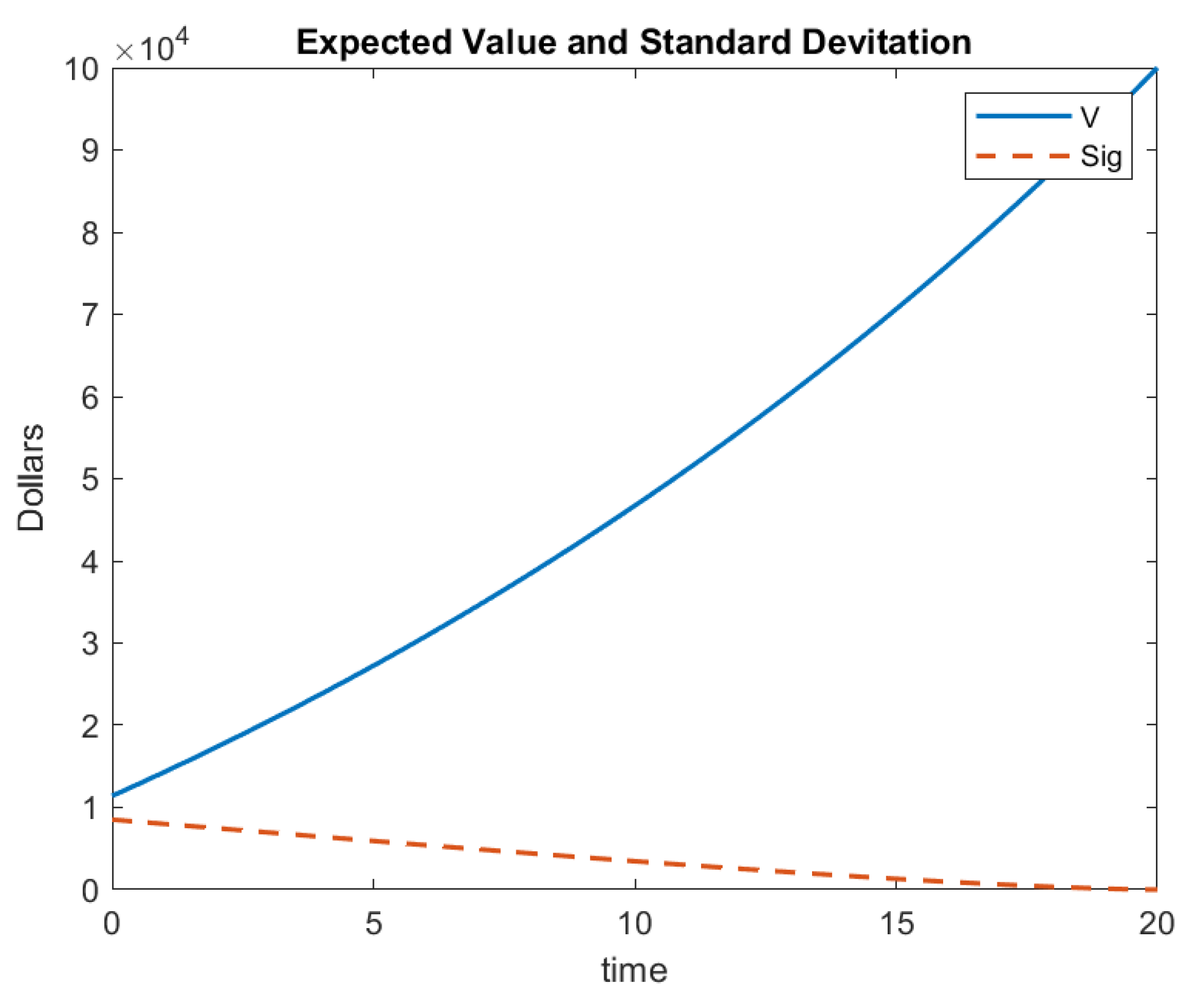
For the first model, a two-state model (alive and dead), we use an example that was found as Example 7.13 in Ref. [1]. In this example, a 20-year endowment insurance is issued to a 30-year-old individual. The value of the policy is USD 100,000, payable immediately upon death or on survival for the entire term, whichever comes first. It is assumed that premiums are payable continuously at a constant rate of USD 2500 per year throughout the term of the policy. The policy uses a constant force of interest, per year, and makes provides no means of recuperating any expenses. In this example, we calculate the value and its standard deviation using the general model that was presented in [12].
Using this information , age = 30, and 100,000, we calculate . Thus, the problem is to solve the system of differential equations:
Using Matlab, the solution is shown in Figure 1.
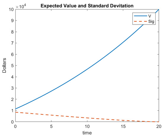
Figure 1.
Example 1 Results.
Additionally,
Note that from this model agrees with that which is calculated in the textbook.
3.2. Example 2: Continuous Time Disability Income Insurance Model
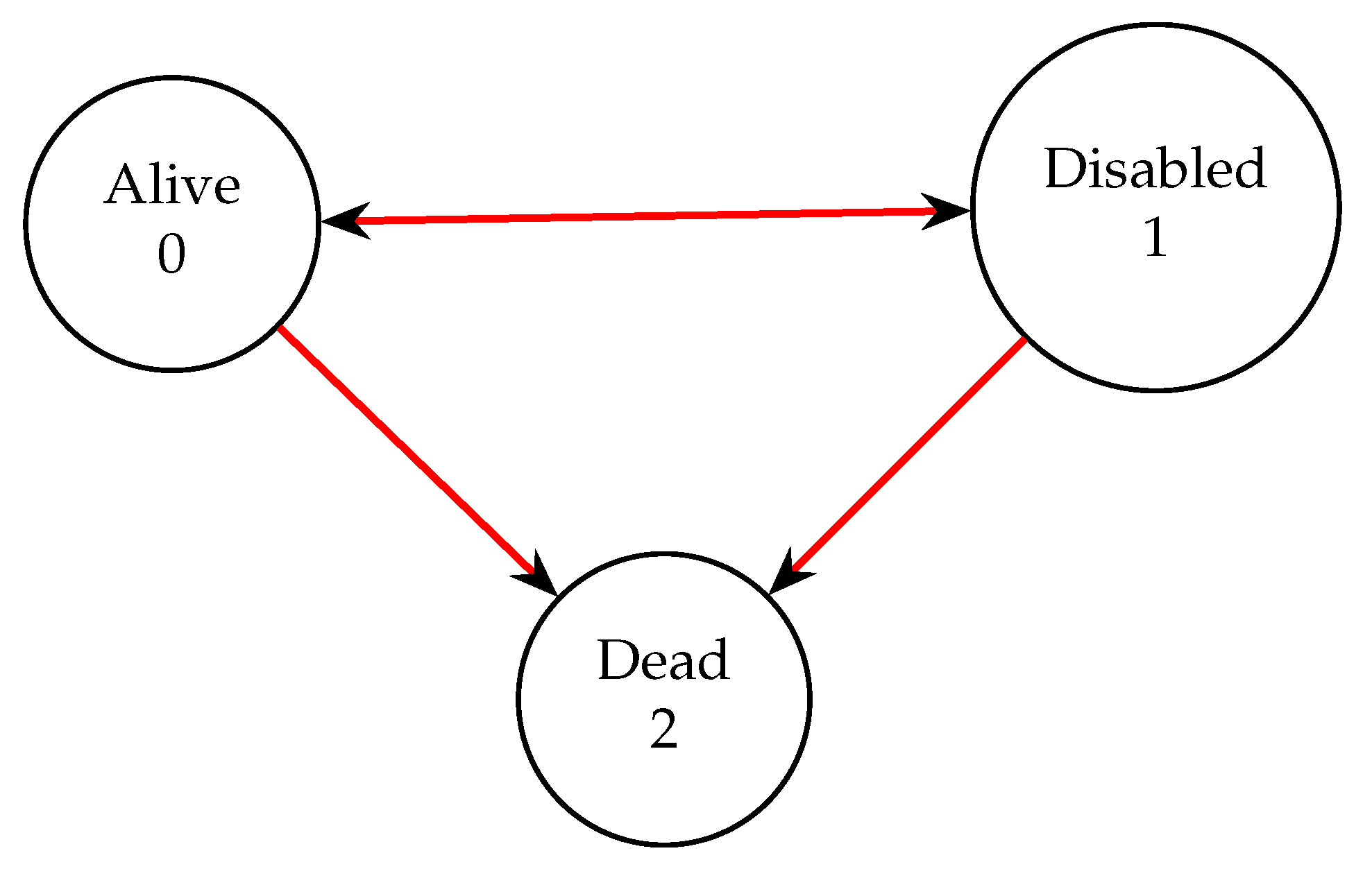
Consider a disability income insurance model with three states—alive, temporary disability, and dead—as shown in Figure 2. We also assume that the following transition rates apply to this example, which was provided, but not solved in [12]:
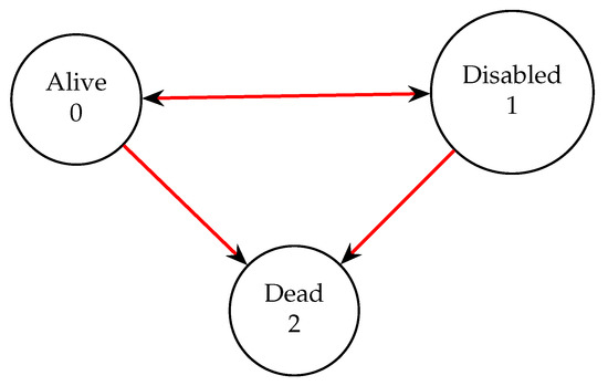
Figure 2.
Example 2 Three State Model.
The valuation force of interest is . We are also given
and
This 10-year health insurance example also has the following assurances.
- -
- The product is issued to a 60-year-old person who is healthy.
- -
- The policy pays a death benefit of USD 5000 at the moment of death.
- -
- The policy includes a continuous disability benefit of USD 750 per year while the insured is temporarily disabled.
- -
- Net premiums are payable continuously while the insured is healthy.
- -
- The policy guarantees an endowment of USD 1000 if the person lives beyond 10 years.
The net premium can be computed using the Equivalence Premium Principle and we assume that value to be P = USD 695.64.
Using this information, Thiele’s differential equation can be written as
Note that for all .
Using this information, Hattendorff’s differential equation for this instance can be presented. Recall that so .
Now,
In addition,
and
Therefore,
The terminal conditions are as follows:
These two systems of differential equations are coupled and they can be solved together. That is, we can combine the systems to obtain
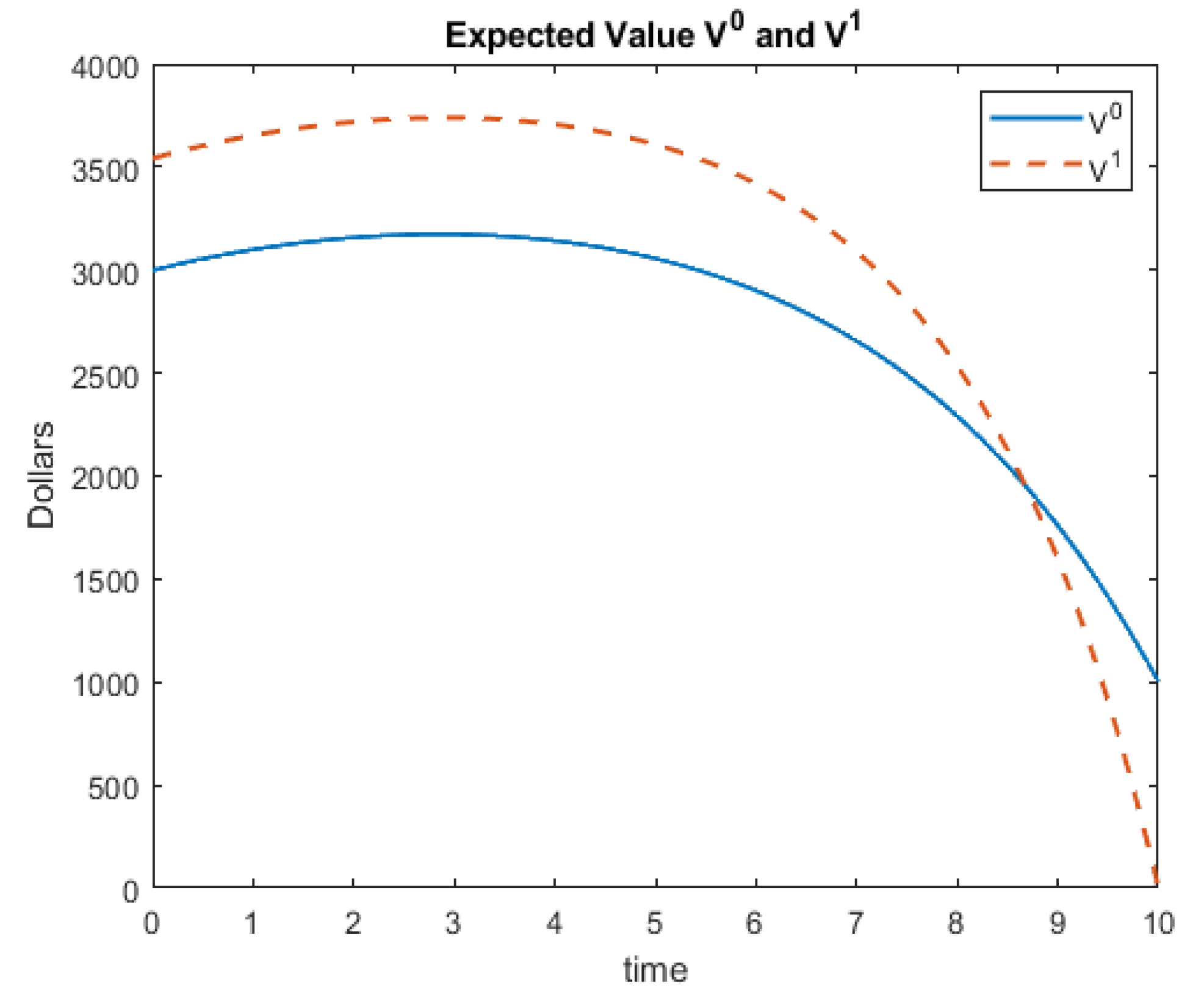
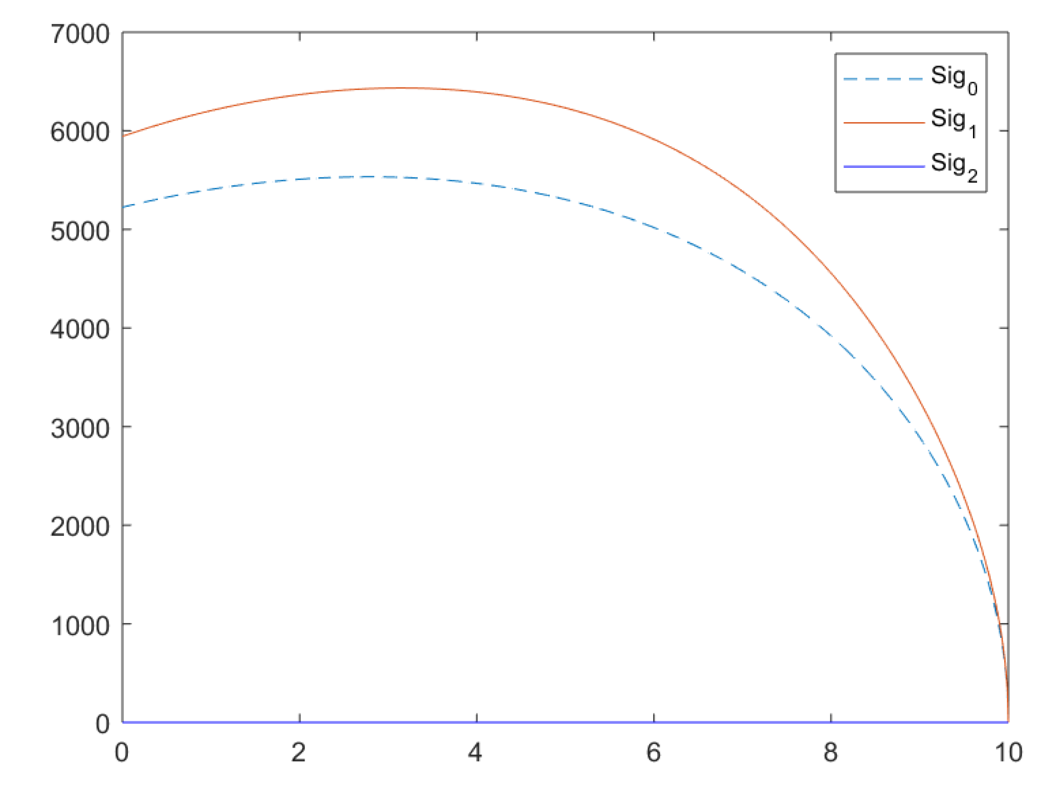
Notice that for these models, we have terminal conditions and not initial conditions. The differential equation solvers that are included with Matlab require initial conditions. Thus, we can simply use the substitution and the chain rule to rewrite the system so that the terminal conditions become initial conditions. Using Matlab’s ‘ode45’ solver, we have the following solutions for this system of differential equations. An identical solution is obtained when the example is presented to Matlab in matrix form. Note that one must rewrite the solution back to the variable t once a solution is obtained. Figure 3 represents the expected values, and Figure 4 represents the standard deviations (square root of the variances) for this example.
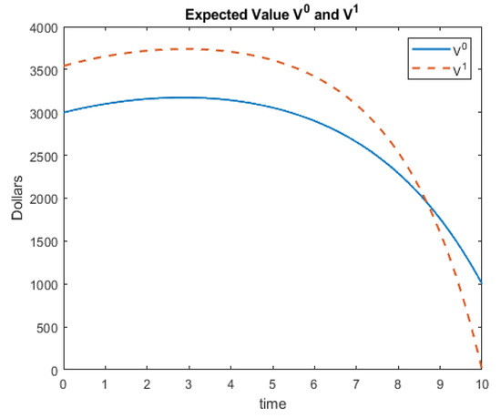
Figure 3.
Example 2 Expected Values.
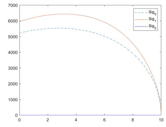
Figure 4.
Example 2 Standard Deviations.
We end the example by stating the following:
- We used Matlab to solve this system of differential equations and acquired both and in the process.
- This step was easily accomplished using Matlab.
3.3. Example 3
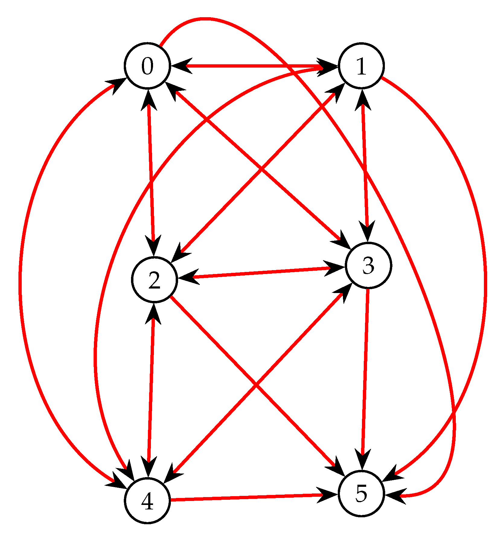
We now consider a six-state insurance model. Consider a disability income insurance model with six states: well (State 0), temporary state of disability (State 1), temporary state of disability 2 (State 2), temporary state of disability 3 (State 3), temporary state of disability 4 (State 4), and dead (State 5), as indicated in Figure 5. We also assume that the following transition rates apply to this example:

Figure 5.
Example 3 Six State Model.
The valuation force of interest is . A 10-year health insurance product has the following features:
- -
- The policy is issued to a 60-year-old person who is healthy.
- -
- The policy guarantees a death benefit of USD 50,000 at the moment of death.
- -
- It also provides a continuous disability benefit at a rate of USD 2500 per year while the insured is temporarily disabled.
- -
- Net premiums are payable continuously while the insured is healthy.
- -
- The policy pays an endowment of USD 5000 if the person lives beyond 10 years.
We are also given enough information to use the equivalence premium principle to calculate for this group, with the assumption that the policy is offered at a rate of
From this information, we have
By Thiele’s differential equation, we have the following:
Note that for all .
In a similar manner, we have the following:
In matrix form, we have
where A and B are used to represent each matrix.
Since for all , no additional differential equations are needed for that particular model.
Now let us consider Hattendorff’s differential equation in matrix form.
Recall that so .
Now,
Substituting in our known values, we have
where C and D are the matrices above. Note that D is in terms of the solution to the first system of equations.
Terminal conditions are as follows:
These two systems of differential equations are coupled and they can be solved together. That is, we can combine the systems to obtain
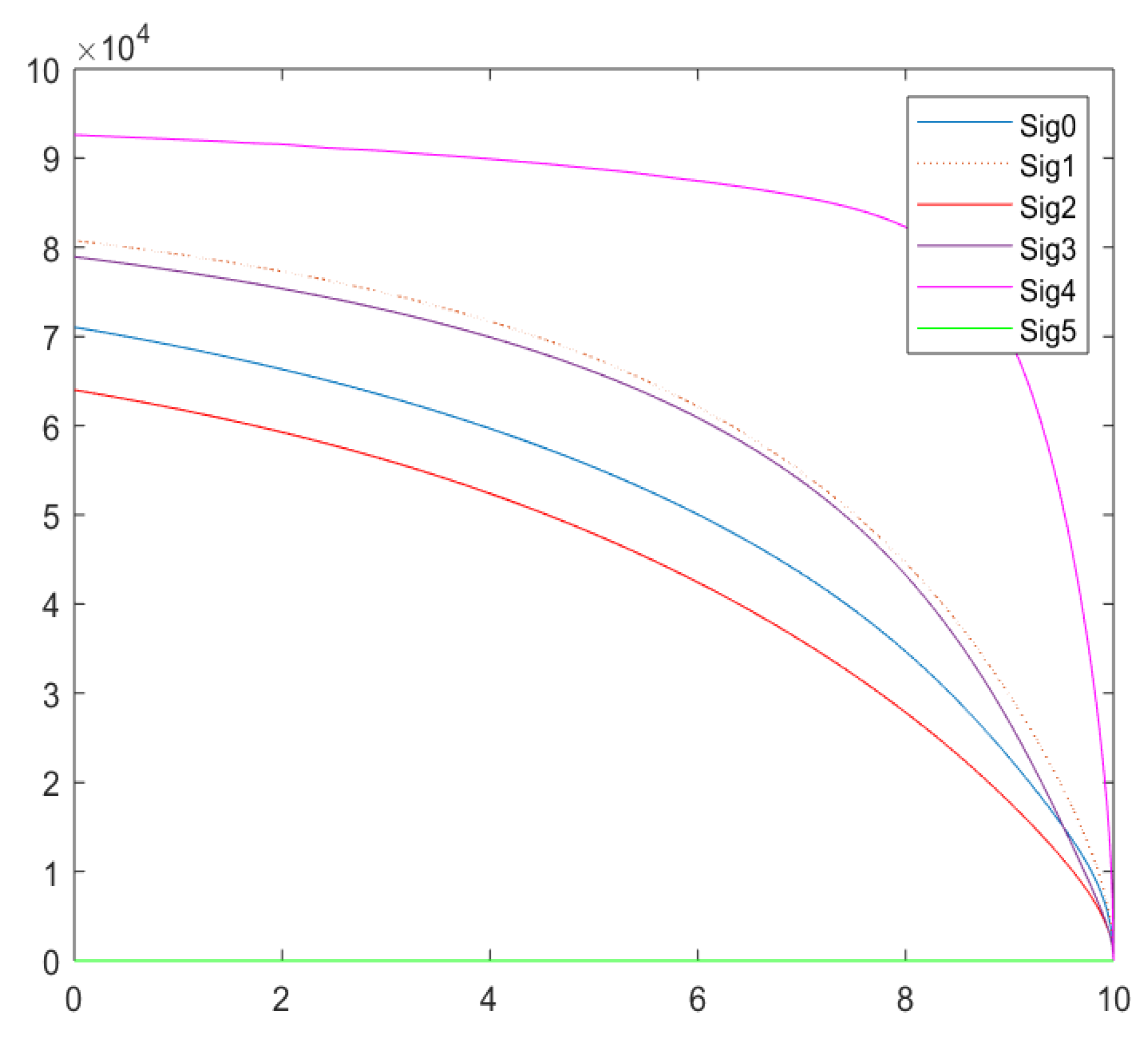
Notice that for these models, we have terminal conditions and not initial conditions. The differential equations solvers that are included with Matlab are designed to require initial conditions. Thus, we can simply use the substitution and the chain rule to rewrite the system so that the terminal conditions become initial conditions. Using the Matlab’s ‘ode45’ solver, we have the following solutions for this system of differential equations. An identical solution is obtained when the example is presented to Matlab in matrix form. Note that one must rewrite the solution back to the variable t once a solution is obtained. Figure 6 represents the expected values and Figure 7 represents the standard deviations (square root of the variances) for this example.
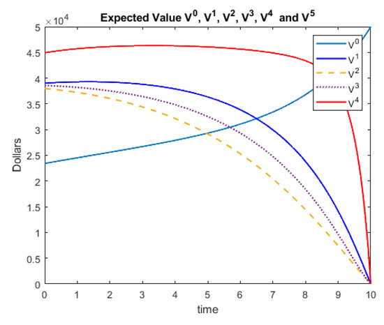
Figure 6.
Example 3 Expected Values.
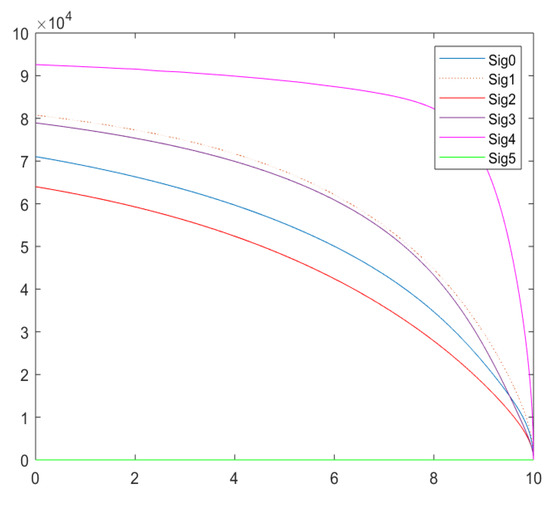
Figure 7.
Example 3 Standard Deviations.
4. Discussion
In this paper, we used the Hattendorff differential equation that we derived in [12], which describes the continuous time evolution of the variance of the loss at time t random variable, given that it is in state j denoted by for continuous cash flows, along with terminal conditions. Matlab was used in three specific examples to numerically solve the Hattendorff differential equation for . The analysis and solution process show the adaptation and closed form expressions for the differential equation and recursion for three examples. Through these examples, we also demonstrated that solutions for various instances of the problem can be easily approximated using Matlab (or similar software). Throughout the demonstrations, advice specific to setting up the Hattendorff differential equation for general multi-state models was given.
More importantly though, the results in this paper provide a numerical algorithm to compute the variance of an insurance product, thus allowing researchers and practitioners to test and simulate various state-space models with multiple diseased and healthy states to test the amount of uncertainty that one can expect in the future loss of the insurance product. Furthermore, it permits the practitioner to compare the evolution of the losses of each multiple-state model, in addition to the evolution of the means (as computed from Thiele’s differential equation), to visually compare and contrast the evolution of the center and spread of the loss variable to glean out practical reasons for unusual changes in the loss. To our knowledge, this is the first time such expressions were used to solve specific instances for the continuous time and discrete time evolution of for the multi-state case.
Author Contributions
Formal analysis, N.R. and R.R. Both authors contributed equally to this paper on everything. All authors have read and agreed to the published version of the manuscript.
Funding
This research received no external funding.
Institutional Review Board Statement
Not applicable.
Informed Consent Statement
Not applicable.
Data Availability Statement
Not applicable.
Conflicts of Interest
The authors declare no conflict of interest.
References
- Bowers, N.L.; Gerber, H.U.; Hickman, J.C.; Jones, D.A.; Nesbitt, C.J. Actuarial Mathematics; The Society of Actuaries: Schaumburg, IL, USA, 1986. [Google Scholar]
- Gerber, H.U. An Introduction to Mathematical Risk Theory; Huebner Foundation, University of Pennsylvania: Philadelphia, PA, USA, 1979. [Google Scholar]
- Gerber, H.U. Lebellsversicherungsmathematik; Springer: Berlin/Heidelberg, Germany; New York, NY, USA, 1986. [Google Scholar]
- Papatriandafylou, A.; Waters, H.R. Martingales in life insurance. Scand. Actuarial J. 1984, 1984, 210–230. [Google Scholar] [CrossRef]
- Ramlau-Hansen, H. Hattendorff’s theorem: A Markov chain and counting process approach. Scand. Actuarial J. 1988, 1987, 143–156. [Google Scholar] [CrossRef]
- Norberg, R. Hattendorff’s theorem and Thiele’s differential equation generalized. Scand. Actuarial J. 1992, 1, 2–14. [Google Scholar] [CrossRef]
- Wolthuis, H. Hattendorff’s theorem for a continuous-time Markov model. Scand. Actuarial J. 1987, 1987, 157–175. [Google Scholar] [CrossRef]
- Norberg, R. Differential Equations for moments of present values in life insurance. Insur. Math. Econ. 1995, 17, 171–180. [Google Scholar] [CrossRef]
- Asmussen, S.; Steffensen, M. Risk and Insurance; Springer: Berlin/Heidelberg, Germany, 2020. [Google Scholar]
- Bladt, M.; Asmussen, A.; Steffensen, S. Matrix representations of life insurance payments. Eur. Actuar. J. 2020, 10, 29–67. [Google Scholar] [CrossRef]
- Hattendorff, K. Das Risiko bei der Lebenversicherung. Masius Rundsch. Versi 1868, 18, 169–183. [Google Scholar]
- Rajaram, R.; Ritchey, N. Hattendorff Differential Equation for Multi-State Markov Insurance Models. Risks 2021, 9, 169. [Google Scholar] [CrossRef]
- Dickson, C.M.D.; Hardy, M.R.; Waters, H.R. Actuarial Mathematics for Life Contingent Risks; Cambridge University Press: Cambridge, UK, 2020. [Google Scholar]

Publisher’s Note: MDPI stays neutral with regard to jurisdictional claims in published maps and institutional affiliations. |
© 2022 by the authors. Licensee MDPI, Basel, Switzerland. This article is an open access article distributed under the terms and conditions of the Creative Commons Attribution (CC BY) license (https://creativecommons.org/licenses/by/4.0/).