Structure of Triangular Numbers Modulo m

Abstract

This work focuses on the structure and properties of the triangular numbers modulo m. The most important aspect of the structure of these numbers is their periodic nature. It is proven that the triangular numbers modulo m forms a $2m$-cycle for any m. Additional structural features and properties of this system are presented and discussed. This discussion is aided by various representations of these sequences, such as network graphs, and through discrete Fourier transformation. The concept of saturation is developed and explored, as are monoid sets and the roles of perfect squares and nonsquares. The triangular numbers modulo m has self-similarity and scaling features which are discussed as well.

1. Introduction

The current work is part of a special issue on the application of number theory in sciences and mathematics and is centered on triangular numbers. More specifically, it is focused on the triangular numbers modulo m, where m is any non-negative integer. Such numbers form a periodic sequence which has an interesting structure. That structure is explored here via elementary number theory, graph theory, and numerical analysis.

The triangular numbers (sometimes called the triangle numbers) are arguably the most well-known of the sequences of polygonal numbers (see [1], chapter 1), which include the square numbers, pentagonal numbers, hexagonal numbers, etc. As the name implies, the polygonal numbers are the sequences formed by counting lattice points cumulatively in subsequent n-gonal patterns. Triangular numbers arise from a triangular lattice. However, triangular numbers are perhaps best known because they represent the cumulative sums of the integers. Each member of the (infinite) sequence of triangular numbers is obtained via a simple closed-form formula per the following definition.

Definition 1.

Triangular numbers. The set of triangular numbers is, for $n\in \mathbb{N}$,

$$\mathcal{T}\equiv \left\{T\left(n\right)=\frac{n(n+1)}{2}\right\}.$$

Note, throughout this work, we are taking $\mathbb{N}$ to include zero (so, the non-negative integers).

The triangular numbers themselves have a long and interesting history [2,3], including the fact that major insight was provided by Gauss himself (see [4], page 91). In spite of all this attention, there is a dearth of literature focused on the triangular numbers mod $m\in {\mathbb{N}}^{+}$ [5]. To be sure, many ideas associated with this set can be found spread through online mathematics communities in forums and blog posts. A number of these ideas, including theorems, are collected in the current work to assist the reader by providing a self-contained presentation. In related work, Wall considered the Fibbonacci numbers modulo m [6] in the early 1960s. Subsequent work on Fibbonicci numbers over cyclic groups was performed by Dikici and coworkers [7,8,9].

The purpose of the current work is to investigate the fascinating structural characteristics of the triangular numbers modulo m. In addition to presenting some new theorems regarding the triangular numbers modulo m, use is made of modern computing power to illustrate some unproven conjectures, which might be useful in applied settings, such as statistical mechanics or computer science. The structure of triangular numbers modulo m reveals a variety of self-similarity and scaling characteristics.

In this work, the designation of a conjecture will be reserved for results in which the author does not have a complete proof. The designation of a proposition will be used for conjecture-like ideas that do have a proof. Lemma, theorem, and corollary designations will be used in their typical ways. Numerical work was done using in-house-made Mathematica and Python code. Network analysis on graphs was done using Gephi.

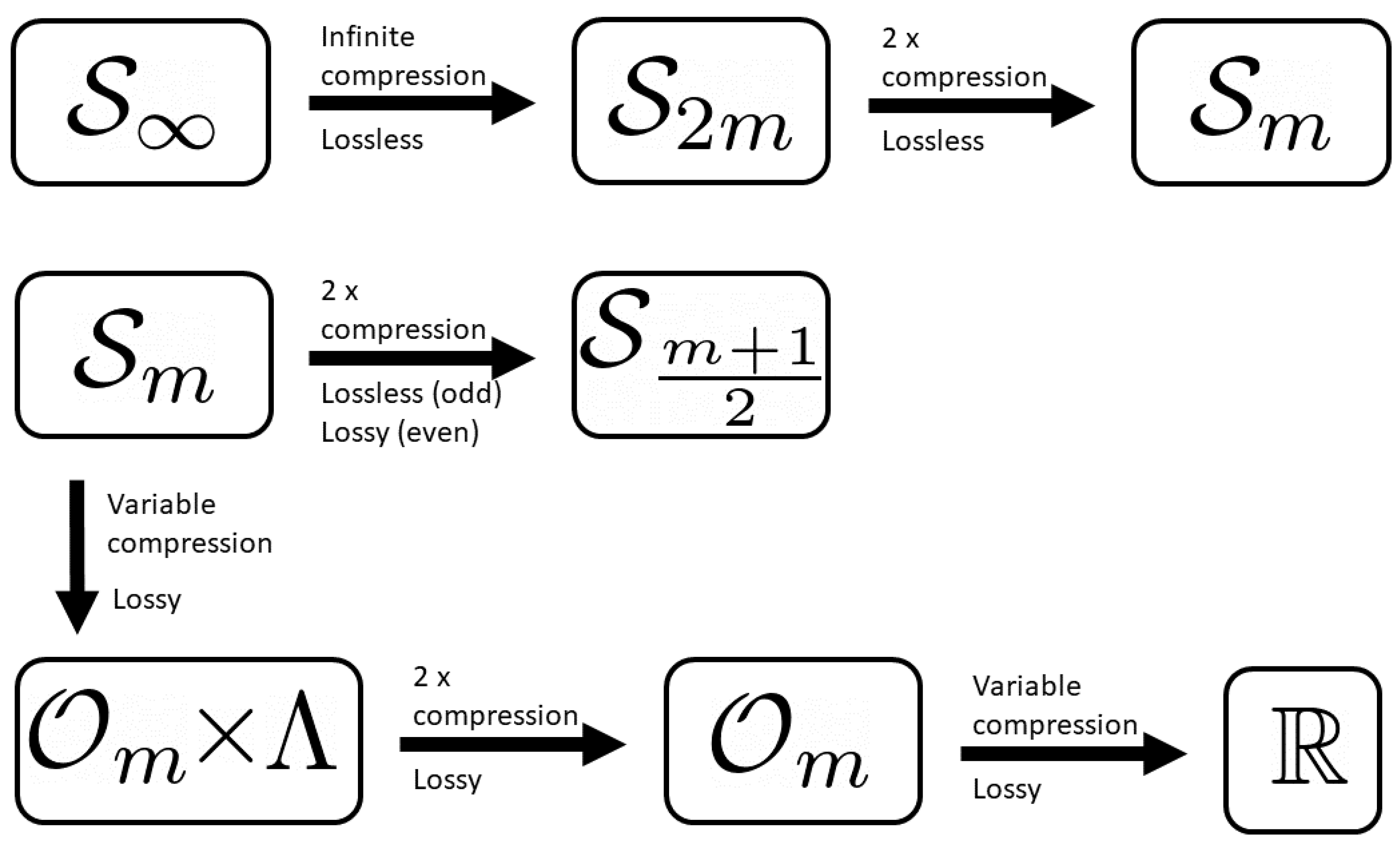
2. Information and Data Compression

Before launching into the details of the structure of the triangular numbers modulo m, this section provides an overarching view of the types of sets one is interested in. Here too, the definitions of the sets are given.

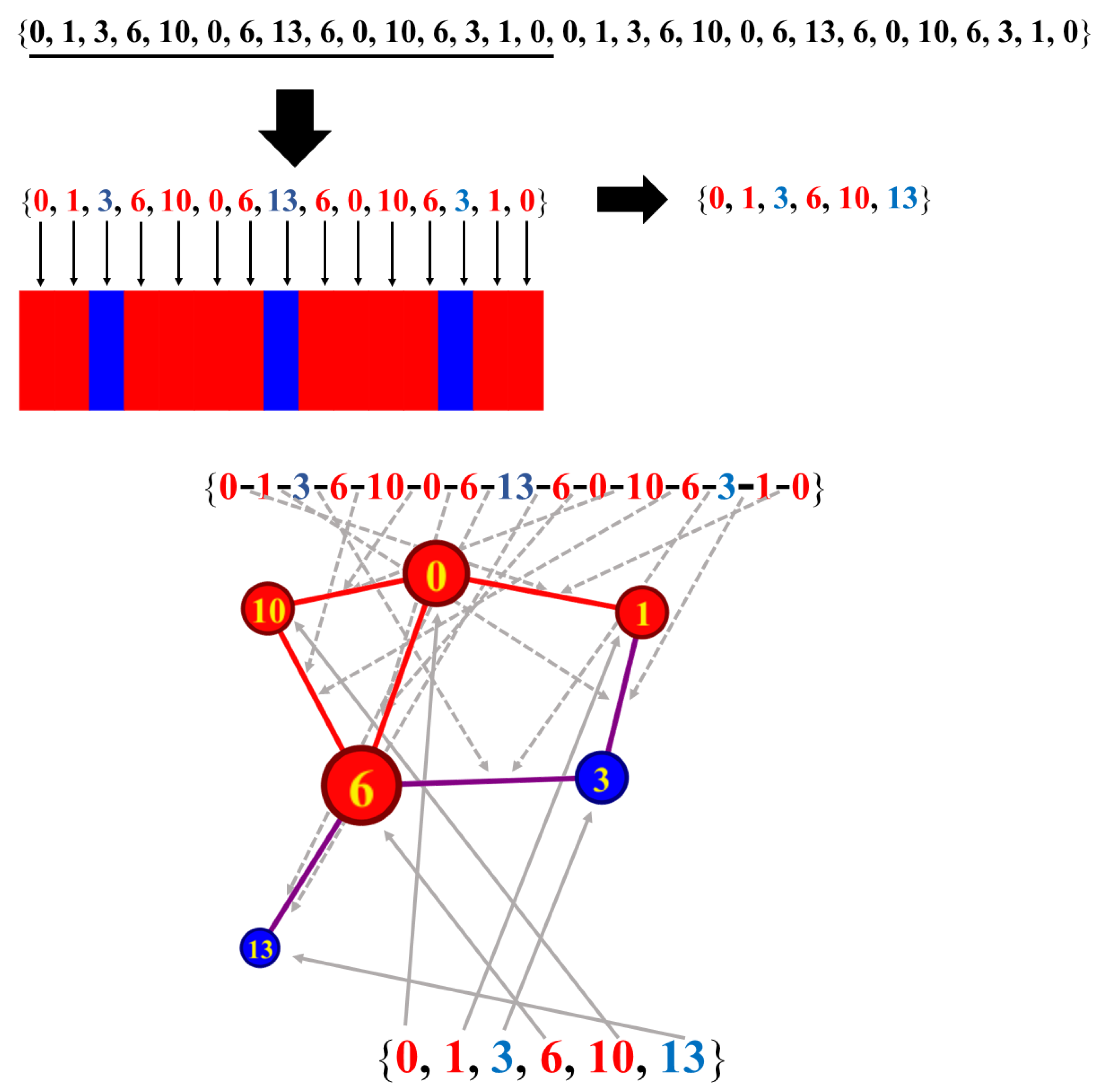
2.1. Sets and Sequences

The triangular numbers themselves, $\mathcal{T}=\{0,1,3,6,10,15,21,28,36,45,55,66,\dots \}$ (series A000217 in the Online Encyclopedia of Integer Sequences [10]) constitute one member of the set of infinite sequences defined here as ${\mathcal{S}}_{\infty }$. Other members of this set include the infinite sequence of the triangular numbers modulo m, $\mathcal{T}modm$. For example, $\mathcal{T}mod6=\{0,1,3,0,4,3,3,4,0,3,1,0,0,1,3,\dots \}$. As mentioned above, the most striking feature of the triangular numbers modulo m is that they are $2m$ periodic for all m. This will be proved (Theorem 1) and discussed more below. This suggests that there is value in naming a family of finite sequences. Each set is labeled ${\mathcal{S}}_{2m}$, representing the specific set of sequences of length $2m$. For a given m, the infinite sequence $\mathcal{T}modm$ maps to a single point in ${\mathcal{S}}_{2m}$.

Definition 2.

The 2m sequence of triangular numbers modulo m.

$${\mathcal{T}}_m\equiv \left\{\mathit{the}\mathit{first}2m\mathit{members}\mathrm{of}\mathcal{T}modm\right\}.$$

Remark 1.

The reader is cautioned to note that the subscript on the element, ${\mathcal{T}}_m$ is m, whereas on the set it is $2m$, ${\mathcal{S}}_{2m}$. This notational inconsistency will pay off in the end because m itself will play such an important role in the current analysis.

There is a natural equivalence class, labeled, $\left[{\mathcal{T}}_m\right]$ in ${\mathcal{S}}_{2m}$, given by the cyclic rotation of the ${\mathcal{T}}_m$. Thus, for example, both elements ${\mathcal{T}}_6=\{0,1,3,0,4,3,3,4,0,3,1,0\}$ and $\{3,1,0,0,1,3,0,4,3,3,4,0\}$ in ${\mathcal{S}}_{2m}$ are members of $\left[{\mathcal{T}}_6\right]$. With a slight abuse of notation, the symbol ${\mathcal{T}}_m$ will represent the equivalence class from here on out. Thus, one is at full liberty to cyclically rotate the sequence as needed.

Two other sets of sets will be important in the current analysis. The first has as elements the set of residue classes present in a given sequence. This is referred to as the set of occupancy set and labeled ${\mathcal{O}}_m$. The point in this set corresponding to ${\mathcal{T}}_m$ is labeled ${\widehat{\mathcal{T}}}_m$. For example, $\widehat{{\mathcal{T}}_6}=\{0,1,3,4\}$. This leads to the following definition

Definition 3.

The occupancy set. ${\widehat{\mathcal{T}}}_m\equiv \left\{\mathit{distinct}\mathit{residues}\mathit{in}{\mathcal{T}}_m\right\}$.

The second set is the set of multiplicity set, labeled, ${\Lambda }_m$, in which each element, ${\Lambda }_m$, is the listing of multiplicities of each member of $\widehat{{\mathcal{T}}_m}$ in the first m (not $2m$) members of ${\mathcal{T}}_m$. As an example, ${\widehat{\lambda }}_6=\{2,1,2,1\}$.

Definition 4.

The multiplicity set ${\widehat{\lambda }}_m\equiv${number of times each distinct residue appears in the first m elements of ${\mathcal{T}}_m$}. Note that the order of the elements in ${\widehat{\lambda }}_m$ corresponds to the order of the elements in ${\widehat{\mathcal{T}}}_m$.

2.2. Information Content of Sets

For the purpose of this work, by “information” we mean how much information is needed to give an explicit listing of a particular sequence. At present, the information unit is generic, but one could, for example, consider the unit as a computer-based calculation unit. Thus, for the triangular numbers themselves, the information needed is infinite (in spite of the closed-form formula). For ${\mathcal{T}}_m$, the amount of information needed is $2m$ units.

Figure 1 shows a schematic representation of the various sets arising in the present analysis. The top row shows the progression from the set of infinite sequences, ${\mathcal{S}}_{\infty }$, to the set of finite sequences of length $2m$. Theorem 1 (proven below) compresses the $2m$-periodic sequence of the triangular numbers modulo m without loss of information. Then, via Theorems 2 and 3, another two-fold compression is achieved by mapping the length $2m$ sequences to the corresponding length m sequences. This is also a lossless mapping due to the nature of the sequences of residue classes as contained in Theorems 2 and 3 (proven below).

The second row of Figure 1 shows the, again, roughly two-fold compression mapping of the sequences of length m to the corresponding sequences of length $\frac{m+1}{2}$. In terms of information loss, we see a divergence between the m in an even case and the m in an odd case. Due to Theorem 4, the odd m case remains lossless. This is not the true for the case when m is an even integer.

The bottom row (along with ${\mathcal{S}}_m$) of Figure 1 shows further compression of information about the sequence of triangular numbers modulo m. All of these mapping are sequentially lossier and lossier, but nonetheless, still lead to sets carrying important information about the sequences. The first map brings the ordered sequence from ${\mathcal{S}}_m$ to the Cartesian product of the occupancy set, ${\mathcal{O}}_m$, and the multiplicity set, $\Lambda$. The data compression here is variable depending on the nature of m. This is discussed in more detail below. Projecting away, the multiplicity set gives two-fold compression. Finally, the definition of saturation, $s=\frac{|{\widehat{\mathcal{T}}}_m|}{|{\mathbb{Z}}_m|}$, gives a representation of the sequence as a single real number $0\le s\le 1$ (formally defined in Definition 5).

3. Main Structure Theorems

The most immediate and critical structural feature of the triangular numbers modulo m is their periodic nature. This is important for a number of reasons but most importantly in reducing an infinite non-repeating sequence to an infinite but repeating sequence of period $2m$. This reduction allows for the properties of this sequence to be studied via a $2m$-member sequence of residue classes. Remarkably, this is the case for any m. Further, theorems dealing with symmetry present in ${\mathcal{T}}_m$ are also given.

The general structure of the triangular numbers modulo m is captured in the following theorems.

3.1. Main Cycle Structure Theorem

Theorem 1.

The sequence of triangular numbers mod m is a $2m$-cycle. Additionally, the sequence is symmetric about the “midpoint” of the $2m$-cycle. That is, the last m elements are the reverse sequence to that of the first m elements.

Proof. 

The $2m$-cycle part. Define $\Delta \equiv T(2m+j)-T\left(j\right)$. Then,

$$\Delta =\frac{(2m+j)(2m+j+1)}{2}-\frac{\left(j\right)(j+1)}{2}.$$

Expansion and simplification leads to

$$\Delta =2m^2+2mj+m.$$

Under modulo m, $\Delta modm=0.$

The symmetry part. Again define a difference, but now $\Delta \equiv T(m+j-1)-T(m-j)$. This is written out as

$$\Delta =\frac{(m+j-1)(m+j)}{2}-\frac{(m-j)(m-j+1)}{2}.$$

Expansion and simplification leads to

$$\Delta =-m+mj.$$

Under modulo m, $\Delta modm=0.$ □

As some concrete examples, ${\mathcal{T}}_{10}=\{0,1,3,6,0,5,1,8,6,5,5,6,8,1,5,0,6,3,1,0\}$ and ${\mathcal{T}}_{15}=\{0,1,3,6,10,0,6,13,6,0,10,6,3,1,0,0,1,3,6,10,0,6,13,6,0,10,6,3,1,0\}$. One sees that the first m elements are all that are required to reconstruct the full sequence without loss of information. That is, the infinite sequences are obtained by repeating these $2m$ sequences indefinitely. For the case of $m=10$, the sequence for the second m elements is the reverse order of the first m because m is even. For $m=15$, where it is odd, the sequence simply repeats as is. The odd/even symmetry behavior will be formally presented in Section 3.2.

Some context is required for the last two sentences of Theorem 1 and the last sentence of the proof. Of course given a ${\mathcal{T}}_m$, one could choose a different member of the equivalence class by starting the cycle at any point, thereby breaking the symmetry, and then the sequence would no longer begin and end with zero. The context here is that the statements about symmetry hold true when the cycle is initiated, with the first member being $T\left(0\right)=0$. There are some situations when it is also natural to initiate the cycle with the first member being $T\left(1\right)=1$. In those situations, the cycle ends with two consecutive zeros.

3.2. Symmetry Theorems

Two related theorems are the following. These deal with the respective symmetries for the odd and even cases.

Theorem 2.

For odd values of m, the triangular numbers’ moduli m form an m-cycle.

Proof. 

As in the previous theorem, define a difference: $\Delta \equiv T(m+j)-T\left(j\right)$. Now one can take advantage of the fact that two has an inverse when m is odd. As such, one can consider

$$2\Delta =(m+j)(m+j+1)-j(j+1).$$

Expansion and simplification leads to

$$2\Delta =m^2+2mj+m.$$

Under modulo m, $2\Delta modm=0.$ This implies $\Delta modm=0$ (because 2 has an inverse) and thus proves the assertion of the theorem. □

The case of ${\mathcal{T}}_{15}$ mentioned above is a concrete manifestation of this theorem. The cases of ${\mathcal{T}}_7=\{0,1,3,6,3,1,0,0,1,3,6,3,1,0\}$ and ${\mathcal{T}}_9=\{0,1,3,6,1,6,3,1,0,0,1,3,6,1,6,3,1,0\}$ serve as further examples, including a prime and a composite.

Theorem 3.

For even values of m, those triangular numbers’ moduli m that are m elements apart in the $2m$-cycle differ by $\frac{m}{2}$.

Proof. 

Again, one defines a difference: $\Delta \equiv T(m+j)-T\left(j\right)$. This is written out as

$$\Delta =\frac{(m+j)(m+j+1)}{2}-\frac{j(j+1)}{2}.$$

Expansion and simplification leads to

$$\Delta =\frac{m^2}{2}+mj+\frac{m}{2}.$$

Writing $\frac{m^2}{2}$ as $m\frac{m}{2}$ and applying modulo m yields $\Delta modm=\frac{m}{2}.$ □

Corollary 1.

The mth member of ${\mathcal{T}}_m$ is $\frac{m}{2}$ when m is even.

Proof. 

The first element of ${\mathcal{T}}_m$ is always zero, so the mth element is $\frac{m}{2}-0=\frac{m}{2}$ via Theorem 3. □

The case of ${\mathcal{T}}_{10}$ mentioned above is an example that falls under Theorem 3 and its corollary. Other examples include the cases of ${\mathcal{T}}_8=\{0,1,3,6,2,7,5,4,4,5,7,2,6,3,1,0\}$ and ${\mathcal{T}}_{12}=\{0,1,3,6,10,3,9,4,0,9,7,6,6,7,9,0,4,9,3,10,6,3,1,0\}$.

Theorem 4.

If m is odd, then ${\mathcal{T}}_m$ is further symmetric about $m^{\prime }=\frac{m-1}{2}$. That is, $T(m^{\prime }-j)=T(m^{\prime }+j)$ where $0<j<m^{\prime }\in {\mathbb{N}}^{+}$.

Proof. 

Define $\Delta \equiv T(m^{\prime }+j)-T(m^{\prime }-j)$. Then, by explicitly writing the triangular summation out and subtracting like terms,

$$\Delta =(m^{\prime }+j)+(m^{\prime }+(j-1))+\dots +(m^{\prime }+1)+m^{\prime }+(m^{\prime }-1)+\dots +(m^{\prime }-(j-1)).$$

Match the terms on the right hand side as

$$\begin{array}{cc}\hfill m^{\prime }+j& +(m^{\prime }+(j-1))+\dots +(m^{\prime }+1)\hfill \\ \hfill & +(m^{\prime }-(j-1))+\dots +(m^{\prime }-1)+m^{\prime }.\hfill \end{array}$$

This gives

$$\begin{array}{cc}\hfill \Delta & =m^{\prime }+j+2(j-1)m^{\prime }+m^{\prime }\hfill \\ \hfill & =2j{m}^{\prime }+j.\hfill \end{array}$$

Substituting in for $m^{\prime }$ gives

$$\Delta =j(m-1)+j=jm.$$

Modulo m gives $\Delta =0.$ □

The working example of ${\mathcal{T}}_{15}$, along with ${\mathcal{T}}_7$ and ${\mathcal{T}}_9$, given the above shows this feature.

Lemma 1.

The triangle numbers’ moduli m are the values of $a\in {\mathbb{Z}}_m$ that give solutions to either of the following two congruence relations: (i) $n(2n+1)=a$ and (ii) $n(2n-1)=a$.

Proof. 

The kth triangle number is given by $\frac{k(k+1)}{2}$. Note that $k(k+1)$ is always even and breaks into two cases. First, when k is even, define $n=\frac{k}{2}$, and thus $T\left(2n\right)=n(2n+1)$. Second, when k is odd, define $n=\frac{k+1}{2}$ and thus $T(2n-1)=n(2n-1)$.

$T\left(k\right)modm$ then becomes $n(2n+1)modm$ or $n(2n-1)modm$. Thus, $n(2n+1)=amodm$ and $n(2n-1)=amodm$ define the congruence relations in ${\mathbb{Z}}_m$ which gives the allowed values of $a\in {\mathbb{Z}}_m$. □

Theorem 5.

The set of unique triangle numbers moduli $m\in {\mathbb{N}}^{+}$, ${\widehat{\mathcal{T}}}_m$, are all $a\in {\mathbb{Z}}_m$ such that $1+8amodm=n^{2}modm$ for some $n\in {\mathbb{Z}}_m$. That is, all a for which $1+8amodm$ is a perfect square under the modulo.

Proof. 

One notes that from Lemma 1, the members of ${\mathcal{T}}_m$ will be all a such that either $n(2n+1)=a$ or $n(2n-1)=a$ yield solutions. It turns out one can more succinctly consider $n(2n\pm 1)=a$ and deal with both congruence relations at once.

Considering the solutions to the quadratic congruence $2n^2\pm n-a=0$, one can write

$$4n=\mp 1\pm \sqrt{(1+8a)}.$$

The important part of this relation is $\sqrt{(1+8a)}$. The set of solutions to the above congruence is given precisely by those values of a in which $1+8a$ is a perfect square under modulo m. This completes the proof. □

At first glance, it seems as though the problem of finding the allowed a might well degenerate into a number of “solvable” cases involving primes, powers of primes, etc., as is often the case when considering quadratic congruences. This is not the case here, however, because one is not looking for a solution to the quadratic congruence per se, but only looking to determine if a particular a yields a solution. These values will be precisely the set listed in Theorem 5.

As an illustrative example of the use of Theorem 5, consider the case of modulo 10. Here the set of perfect squares are $\left\{0,1,4,5,6,9\right\}$, and the set of ordered pairs is $(a,1+8amod10)=\left\{(0,1),(1,9),(2,7),(3,5),(4,3),(5,1),(6,9),\right.$$\left.(7,7),(8,5),(9,3)\right\}$. The intersection of the perfect square set and the set of $1+8a$ values is $\left\{1,5,9\right\}$. These values correspond to the set of a values $\left\{0,1,3,5,6,8\right\}$. Thus, ${\widehat{\mathcal{T}}}_{10}=\left\{0,1,3,5,6,8\right\}$. These are indeed the values that appear for the triangular numbers modulo 10.

It is also noteworthy that Theorem 5 does not have a great deal of power in the applied setting because it does not give a specific mechanism for finding which a make up ${\widehat{\mathcal{T}}}_m$, nor does it give the multiplicity of a. That is, ${\widehat{\mathcal{T}}}_m$ loses information about the ordered set ${\mathcal{T}}_m$. Finally, Section 7.2 takes a closer look at perfect squares and their relation to the members of ${\widehat{\mathcal{T}}}_m$.

Theorem 6.

If m is even, there are equal numbers of even and odd numbers in the first m members of the $2m$-cycle of Theorem 1.

Proof. 

Let $m=2n$ and consider the size $2n$ set

$$A=\left(\left\{\frac{(2n-j-1)(2n-j)}{2}\right\}mod2\right)$$

for $j=0$ to $j=2n-1$. The role of modulo 2 is to make A simply a set of even (0) and odd (1) numbers. Expanding the above expression gives

$$A=\left(\left\{2n^2+2nj-n+\frac{j(j+1)}{2}\right\}mod2\right).$$

The first two terms vanish under the mod. Considering $\frac{j(j+1)}{2}mod2$ and Theorem 1 yields the 4-cycle $\{0,1,1,0,\mathrm{repeat}\}$. Regardless of whether n is 1 or 0, there are the same numbers of even and odd entries in set A. □

Consider the case of ${\mathcal{T}}_8$, ${\mathcal{T}}_{10}$, and ${\mathcal{T}}_{12}$ given earlier. Indeed there are 4, 5, and 6 evens, respectively, and the same for odds.

4. Specific Structure Theorems

Some specific characteristics of the structure of the triangular numbers mod m are discussed here. First, the case of $m=2^j$, where $j\in {\mathbb{N}}^{+}$. Then, the cases in which m is prime or prime power are presented.

4.1. Theorems Related to $m=2^n$

Theorem 7.

If $m\ne 2^n$ and $n\in {\mathbb{N}}^{+}$, then the first time 0 reappears is at a position less than or equal to the $m-1$ position. The converse is also true.

Proof. 

Write $m=2^{j}c$ and observe that $2^j$ and c are relatively prime. Consequently, the Chinese remainder theorem implies that there exists a nonzero $a\in {\mathbb{N}}^{+}$ such that $amod{2}^{j+1}=0$ and $amodc=-1$ and that a is uniquely determined modulo $2^{j+1}c$. Since $2^{j+1}c=2m$, $0<a\le 2m-1$. Now, $amod{2}^{j+1}=0$ and $a+1modc=0$. Thus, $a(a+1)mod{2}^{j+1}c=a(a+1)mod2m$. This implies $\frac{a(a+1)}{2}modm=0$. This leads to two cases: (i) $0<a\le m-1$, so $T\left(a\right)modm=0$ directly. (ii) $m<a\le 2m-1$. Here one can define $b=2m-1-a$ so that $0<b\le m-1$. Then,

$$\begin{array}{cc}\hfill T\left(b\right)modm& =\frac{b(b+1)}{2}modm\hfill \\ \hfill & =\frac{(2m-1-a)(2m-a)}{2}modm\hfill \\ \hfill & =\frac{4m^2-2m-4am+a+a^2}{2}modm\hfill \\ \hfill & =\left(2m^2-m-2am+\frac{a(a+1)}{2}\right)modm=0.\hfill \end{array}$$

Finally, $c=a$ or b appropriately such that $0<a\le m-1$ and $T\left(c\right)modm=0$.

The converse follows quickly because if 0 reappears prior to the $m-1$ position in the sequence, then it has appeared at least twice overall (the first time being at position 0 itself). Then, by Theorem 8, $m\ne 2^n$, as is shown next. □

The working examples of $T_{10}$ and $T_{15}$ bear this out. For $T_{10}$ zero reappears at position 5, and for $T_{15}$ it reappears at position 6.

Theorem 8.

All values of ${\mathbb{Z}}_m$ appear once and only once in the first m members of the $2m$-cycle if and only if $m=2^n$, $n\in \mathbb{N}$.

Proof. 

The if part of the proof will be by induction. In general, one is given that $m=2^n$. For the base case $m=2$ and under these conditions, $T\left(i\right)modm=0$ or 1. Hence, the base case is true. One then assumes it is true that all values appear once and only once in the first m members of the $2m$-cycle if $m=2^j$ and one considers the case when $n=j+1$.

Let $m=2^j$ and $a,b\in \mathbb{Z}$ such that $0\le a\le m-1$ and $b=2m-1-a$. This implies $m\le 2b+1$. Now define $\Delta \equiv T\left(b\right)-T\left(a\right)$. Then,

$$\begin{array}{cc}\hfill \Delta & =\frac{b(b+1)}{2}-\frac{a(a+1)}{2}\hfill \\ \hfill & =\frac{(2m-1-a)(2m-a)-a(a+1)}{2}\hfill \\ \hfill & =\frac{4m^2-2m-4ma+a+a^2-a^2-a}{2}\hfill \\ \hfill & =2m^2-m-2ma.\hfill \end{array}$$

Now $\Delta modm=0$ and thus $T\left(b\right)=T\left(a\right)$ for all $0\le a\le m-1$ modulo m and by the assumption of the jth inductive step, all values appear once and only once. However, $\Delta mod2m\ne 0$ for all $0\le a\le m-1$. Since $m\le 2b+1$, all new values up to $2m-1$ must appear once and only once. As $2m=m^{j+1}$, this completes the if part of the proof.

The only if part follows from Theorem 7, given all values appear once and only once in the first m members of the $2m$-cycle. Let $m=2^j{m}^{\prime }$; then, by Theorem 7, there exists an a such that $0<a\le m-1$ and $T\left(a\right)modm=0$. However, 0 is also the first value. This poses a contradiction and completes the proof. □

As a concrete example, ${\mathcal{T}}_8=\{0,1,3,6,2,7,5,4,4,5,7,2,6,3,1,0\}$. One sees that each residue appears in the first 8 elements and then again in the second 8 elements.

Corollary 2.

If $m\ne 2^n$, then at least one value has a multiplicity greater than one (appears more than once). The converse is also true.

Proof. 

Follows immediately from the pigeonhole theorem, and the converse follows from Theorem 8. □

4.2. Theorems Involving Cases When m Is Prime

Lemma 2.

If m is prime, then $T\left(a\right)modm\ne 0$ for $0<a<m-1$.

Proof. 

Assume $T\left(a\right)=\frac{a(a+1)}{2}=0modm$. As m is prime, ${\mathbb{Z}}_m$ is a field. Together, this implies either $a=cm$ or $(a+1)=cm$, where $c\in \mathbb{Z}$. However, this contradicts the stipulation on a in the theorem. □

Theorem 9.

If m is an odd prime, then $T\left(a\right)\ne T\left(b\right)$ for $a<b\le \frac{m-1}{2}$.

Proof. 

Begin with $\Delta \equiv T\left(b\right)-T\left(a\right)$, and since m is odd, we can consider $2\Delta =2T\left(b\right)-2T\left(a\right)$. Writing out the triangle numbers gives

$$\begin{array}{cc}\hfill 2\Delta & =b^2+b-a^2-a\hfill \\ \hfill 2\Delta & =b^2-a^2+b-a.\hfill \end{array}$$

Expanding and factoring out a $b-a$ yields

$$2\Delta =(b+a)(b-a+1).$$

The imposed limits on a and b ensure $(a+b)\ne m$ and $(b-a+1)\ne 0$. Further, because m is prime, ${\mathbb{Z}}_m$ is a field; thus, $\Delta \ne 0.$ This completes the proof. □

Theorem 10.

If m is an odd prime, then $T\left(a\right)\ne T(a+1)$ for $0<a<m-1$.

Proof. 

Since m is odd, two has an inverse. Thus, one considers $2T\left(a\right)=a(a+1)$ and $2T(a+1)=(a+1)(a+2)$. These terms share $(a+1)$ as a factor. Consequently, $2T\left(a\right)$ and $2T(a+1)$ must lie in either the same row or same column of the multiplication Caley table ([11], page 43). Since ${\mathbb{Z}}_m$ is a field (multiplication in ${\mathcal{Z}}_m^{+}$ forms a group), $T\left(a\right)\ne T(a+1)$. □

As a concrete example, consider ${\mathcal{T}}_{11}=\{0,1,3,6,10,4,10,6,3,1,0,0,1,3,6,10,4,10,6,3,1,0\}$. Here we see no two consecutive residues are the same until the two zeros.

4.3. Theorems Involving Cases When m Is a Prime Squared

Lemma 3.

For $m=p^2$, where p is an odd prime, $T\left(\frac{p-1}{2}\right)=T\left(ap+\frac{p-1}{2}\right)mod{p}^2$ for all $a\in \mathbb{N}$.

Proof. 

We start with

$$\begin{array}{cc}\hfill T\left(ap+\frac{p-1}{2}\right)& =\frac{\left(ap+\frac{p-1}{2}\right)\left(ap+\frac{p-1}{2}+1\right)}{2}mod{p}^2\hfill \\ \hfill & =\frac{\left(ap+\frac{p-1}{2}\right)\left(ap+\frac{p+1}{2}\right)}{2}mod{p}^2\hfill \\ \hfill & =\frac{a^2{p}^2}{2}+\frac{ap}{2}\left(\frac{p-1}{2}\right)+\frac{ap}{2}\left(\frac{p+1}{2}\right)+\frac{1}{2}\left(\frac{p-1}{2}\right)\left(\frac{p+1}{2}\right)mod{p}^2\hfill \\ \hfill & =\frac{a^2{p}^2}{2}+\frac{a{p}^2}{4}-\frac{ap}{2}+\frac{a{p}^2}{2}+\frac{ap}{4}+\frac{1}{2}\left(\frac{p-1}{2}\right)\left(\frac{p-1}{2}+1\right)mod{p}^2\hfill \\ \hfill & =\frac{a^2{p}^2}{2}+\frac{a{p}^2}{2}+T\left(\frac{p-1}{2}\right)mod{p}^2.\hfill \end{array}$$

Now one must consider the cases when a is even and odd. If $a=2b$ is even,

$$\begin{array}{cc}\hfill T\left(ap+\frac{p-1}{2}\right)& =\frac{4b^2{p}^2}{2}+\frac{2b{p}^2}{2}+T\left(\frac{p-1}{2}\right)mod{p}^2\hfill \\ \hfill & =2b^2{p}^2+b{p}^2+T\left(\frac{p-1}{2}\right)mod{p}^2\hfill \\ \hfill & =T\left(\frac{p-1}{2}\right)mod{p}^2.\hfill \end{array}$$

If $a=2b+1$ is odd,

$$\begin{array}{cc}\hfill T\left(ap+\frac{p-1}{2}\right)& =\frac{4b^2{p}^2}{2}+\frac{4b{p}^2}{2}+\frac{p^2}{2}+\frac{2P^2}{2}+\frac{p^2}{2}+T\left(\frac{p-1}{2}\right)mod{p}^2\hfill \\ \hfill & =2b^2{p}^2+2b{p}^2+\frac{4p^2}{2}+T\left(\frac{p-1}{2}\right)mod{p}^2\hfill \\ \hfill & =T\left(\frac{p-1}{2}\right)mod{p}^2.\hfill \end{array}$$

This proves the lemma. □

As a concrete example, consider ${\mathcal{T}}_{25}=\{0,1,3,6,10,15,21,3,11,20,5,16,3,16,5,20,11,3,21,15,10,6,3,1,0,0,1,3,6,10,15,21,3,11,20,5,16,3,16,5,20,11,3,21,15,10,6,3,1,0\}$. One sees here that the residue three occurs at position $\frac{5+1}{2}$ and is repeated every five thereafter.

Theorem 11.

For $m=p^2$ where p is an odd prime, residues appear only once in the first $\frac{m+1}{2}$, except for the residue class equivalent to $T\left(\frac{p-1}{2}\right)$, which appears exactly $\frac{p+1}{2}$ times.

Proof. 

It is convenient to consider residues centered on $\frac{p-1}{2}$. Define $\Delta =T\left(\frac{p-1}{2}+r_1\right)-T\left(\frac{p-1}{2}+r_2\right)$. Without loss of generality, one can take $r_1>r_2$. Writing out $\Delta$ and simplifying gives

$$\begin{array}{cc}\hfill \Delta & =\frac{\left(\frac{p-1}{2}+r_1\right)\left(\frac{p-1}{2}+r_1+1\right)}{2}-\frac{\left(\frac{p-1}{2}+r_2\right)\left(\frac{p-1}{2}+r_2+1\right)}{2}\hfill \\ \hfill & =\frac{(r_1-r_2)(p+r_1+r_2)}{2}.\hfill \end{array}$$

One can immediately pick up the last statement of the theorem by setting $r_2=0$. Then,

$$\begin{array}{c}\hfill \Delta =\frac{r_1(p+r_1)}{2},\end{array}$$

which equals zero modulo $p^2$ if and only if $r_1=jp$. The if part of the theorem comes directly with substitution and hence proves the last statement. The only if part of the theorem comes from the fact that for $\Delta =0mod{p}^2$$r_1(p+r_1)=a{p}^2$, but the only factors in $a{p}^2$ are a and p and the factors on the left-hand side are not those.

To get the first part of the statement, one makes two steps. First, make the restriction, $r_1=x+jp$ and $r_2=y+jp$, such that $0<y<x<p$. This will scan the range between $\frac{p-1}{2}+jp$ and $\frac{p-1}{2}+(j+1)p$. Here,

$$\begin{array}{c}\hfill \Delta =T\left(\frac{p-1}{2}+jp+x\right)-T\left(\frac{p-1}{2}+jp+y\right)=\frac{(x-y)(2jp+p+x+y)}{2}.\end{array}$$

Now define $v\equiv x-y$ and $u\equiv x+y$. Note that $0<v<p$. Finally, denote the multiplicative inverse of two, which exists under modulo $p^2$, as $2^{-}$. This gives,

$$\begin{array}{cc}\hfill \Delta & =2^{-}v(2jp+p+u).\hfill \end{array}$$

Given that $2^{-}\ne p$, $\Delta$ cannot be zero modulo $p^2$ for $v\ne 0$, which is the case for v. Thus, $T\left(\frac{p-1}{2}+jp+x\right)\ne T\left(\frac{p-1}{2}+y+jp\right)modm$.

The last step is to show that no two resides that differ by multiples of p are equal in the first $\frac{m+1}{2}$ members of the sequence. Again define the difference, $\Delta =T\left(\frac{p-1}{2}+r+jp\right)-T\left(\frac{p-1}{2}+r+kp\right)$. Then,

$$\begin{array}{cc}\hfill \Delta & =\frac{\left(jp+\frac{p-1}{2}+r\right)\left(jp+\frac{p-1}{2}+r+1\right)}{2}-\frac{\left(kp+\frac{p-1}{2}+r\right)\left(kp+\frac{p-1}{2}+r+1\right)}{2}\hfill \\ \hfill & =p^2\left(\frac{j^2}{2}+\frac{j}{2}\right)+jpr-p^2\left(\frac{k^2}{2}-\frac{k}{2}\right)-kpr.\hfill \end{array}$$

Upon modulo $p^2$, the first and third terms go to zero.

$$\begin{array}{cc}\hfill \Delta & =\frac{\left(jp+\frac{p-1}{2}+r\right)\left(jp+\frac{p-1}{2}+r+1\right)}{2}-\frac{\left(kp+\frac{p-1}{2}+r\right)\left(kp+\frac{p-1}{2}+r+1\right)}{2}\hfill \\ \hfill & =(j-k)pr.\hfill \end{array}$$

Now, for $\Delta$ to be zero modulo $p^2$, $(j-k)r=p$ but p is prime. Thus, if $(j-k)=1$, that would require $r=p$ but $r<p$. Likewise, if $r=1$.

Thus, these combined facts, along with Theorem 4, which states that the first $\frac{m+1}{2}$ elements fully determine ${\mathcal{T}}_m$, complete the first statement of the theorem. □

5. Property Theorems

Several properties of the triangular numbers modulo m are collected and discussed in this section.

Theorem 12.

If m is even, then $\left(T\right(k)+T(k+1\left)\right)=\left(T\right(k+m)+T(k+m+1\left)\right)modm$.

Proof. 

As has been done often prior, define

$$\Delta \equiv T(k+m)+T(k+m+1)-T\left(k\right)+T(k+1).$$

Writing everything out and simplifying gives

$$\Delta =m^2+2mk+2m.$$

Applying modulo m gives $\Delta =0$ and completes the proof. □

Theorem 13.

If m is odd, $0\le a\le \frac{m-1}{2}$, and $b=m-1-a$, then $T\left(b\right)=T\left(a\right)modm$.

Proof. 

That m is odd implies that two has an inverse. With that, the direct route is taken. Upon substitution,

$$2T\left(b\right)=b(b+1)$$

leads to

$$2T\left(b\right)=(m-1-a)(m-a).$$

Expanding and simplifying gives

$$2T\left(b\right)=m(m-1)+ma+a(a+1),$$

which becomes $2T\left(b\right)=2T\left(a\right)$ under modulo m. Since two has an inverse, the proof is completed. □

Consider the concrete example of ${\mathcal{T}}_{15}$ and pick a to be 3; then, $b=15-1-3=11$. Now, $T\left(3\right)=6mod15$ and $T\left(11\right)=6mod15$. The reader can pick other values of a.

Theorem 14.

If $m=q^2$ where q is odd, then $T\left(\frac{q-1}{2}\right)modm=T\left(\frac{q-1}{2}+jq\right)modm$, where $j\ge 0\in \mathbb{Z}$.

Proof. 

Noting that m must be odd and using the fact that two has an inverse, the direct route is taken.

$$\begin{array}{cc}\hfill 2T\left(\frac{q-1}{2}+jq\right)& =\left(\left(\frac{q-1}{2}\right)+jq\right)\left(\left(\frac{q-1}{2}\right)+jq+1\right)\hfill \\ \hfill & ={\left(\frac{q-1}{2}\right)}^2+\left(\frac{q-1}{2}\right)+2jq\left(\frac{q-1}{2}\right)+jq+{\left(jq\right)}^2\hfill \\ \hfill & ={\left(\frac{q-1}{2}\right)}^2+\left(\frac{q-1}{2}\right)+jq(q-1)+jq+q^2{j}^2.\hfill \end{array}$$

The first two terms constitute $2T\left(\frac{q-1}{2}\right)$, and the last three become $q^2(j+j^2)$, which vanish under modulo $m=q^2$. Thus,

$$2T\left(\frac{q-1}{2}+jq\right)=2T\left(\frac{q-1}{2}\right),$$

and multiplying by two’s inverse completes the proof. □

Theorem 15.

If m is even, then $T(m-1)modm=m/2$.

Proof. 

The direct route is taken.

$$\begin{array}{cc}\hfill T(m-1)& =\frac{(m-1)m}{2}modm\hfill \\ \hfill & =\frac{m^2}{2}+\frac{-m}{2}modm\hfill \\ \hfill & =m\frac{m}{2}+\frac{-m}{2}modm\hfill \\ \hfill & =0+\frac{m}{2}.\hfill \end{array}$$

This completes the proof. □

Theorem 16.

For $m=2q$ where q is odd.(a)$T\left(q\right)modm=0$ if $m=4n-1$ and (b)$T(q-1)modm=0$ if $q=4n+1$.

Proof. 

Both (a) and (b) will be proven simultaneously. Let $a=m-j$, where $-q<j<q$. Then, by Theorem 7, one can certainly set $T(q-j)modm=0$. One then solves for j:

$$\begin{array}{cc}\hfill 0& =T(q-j)modm\hfill \\ \hfill & =\frac{(q-j)(q-j+1)}{2}modm\hfill \\ \hfill & =\frac{q^2+q-2qj+j^2-j}{2}modm\hfill \\ \hfill & =\frac{q(q+1)}{2}+qj+\frac{j(j-1)}{2}modm.\hfill \end{array}$$

For this relation to hold for any q, either $j=0$ or $j=1$, because the last term must always vanish. These give the two cases $T\left(q\right)modm=0$ and $T(q-1)modm=0$, respectively.

Consider the first case. This implies

$$\frac{\left(q\right)(q+1)}{2}=nm.$$

Since $m=2q$, $q(q+1)=4nq$. Solving for q gives $q=4n-1$, which proves case (a).

Consider the second case. This implies

$$\frac{(q-1)q}{2}=nm.$$

Since $m=2q$, $(q-1)q=4nq$. Solving for q gives $q=4n+1$, which proves case (b). □

Corollary 3.

In Theorem 16 for case (a)$T(q-1)=q$ and $T(q+1)modm=q+1$, and for case (b)$T(q-2)=q+1$ and $T\left(q\right)modm=q$.

Proof. 

Case (a). $0=T\left(q\right)=\left(T\right(q-1)+q)modm$. Thus, $T(q-1)=q$. Additionally, $0=T\left(q\right)m=\left(T\right(q+1)-(q+1\left)\right)modm$. Thus, $T(q+1)modm=q+1$.

Case (b). $0=T(q-1)modm=\left(T\right(q)-q)modm$. Thus, $T\left(q\right)modm=q$. Additionally, $0=T(q-1)modm=\left(T\right(q-2)+(q-1\left)\right)modm$. Thus, $T(q-2)modm=q+1$. □

6. Saturation Theorems

The scheme of information compression captured in Figure 1 ultimately compresses the triangular numbers modulo m down to a single real number between 0 and 1. This parameter, s, is called saturation. While much information is lost from the original sequence, the behavior of saturation with m still possesses very interesting features.

Definition 5.

Saturation. The saturation, $s_m=\frac{|\widehat{{\mathcal{T}}_m}|}{|{\mathbb{Z}}_m|}$.

Figure 2 shows the saturation values as a function of m for m ranging up to 700,000. One immediate feature of the plot is the presence of striations of heavily populated s values and regions of sparse values. One notices sequences of points converging into asymptotic values—for example, $s=\frac{1}{2}$, etc. There are also sequences of constant s values that increase in distance between points—for example, $s=1,0.6$, etc. A blow-up of the small s values is shown in the bottom graph of Figure 2. One sees a “dripping” of single points falling below the main cloud of points. The following theorems, propositions, and conjectures describe these features.

Proposition 1.

The saturation $s_m=1$, when $m=2^n$.

Proof. 

This follows immediately from Theorem 8. □

This proposition explains the sequence of points with increasing spacing at a value of $s=1$.

Proposition 2.

The saturation of ${\mathcal{T}}_m$, where $m=p$ an odd prime, is $s_p=\frac{p+1}{2p}$.

Proof. 

From Theorem 9 the residues, $0\le r\le \frac{p-1}{2}$, determines the sequence for $m=p$, where p is an odd prime. From Theorem 4, the first $\frac{p+1}{2}$ members are distinct from one another. Thus,

$$s_p=\frac{\frac{p+1}{2}}{p}=\frac{p+1}{2p},$$

which proves the proposition. □

For example, ${\widehat{\mathcal{T}}}_{11}=\{0,1,3,4,6,10\}$ so $s_{11}=\frac{6}{11}$. By Proposition 2, $s_{11}=\frac{11+1}{2·11}=\frac{6}{11}$.

Proposition 3.

The saturation of ${\mathcal{T}}_m$, where $m=p$ is an odd prime, goes to $s_p=\frac{1}{2}$ in the limit of a large p.

Proof. 

From Proposition 2,

$$\underset{p\to \infty }{lim}{s}_p=\underset{p\to \infty }{lim}\frac{p+1}{2p}=\frac{1}{2}.$$

This completes the proof. □

Propositions 2 and 3 describe the sequence of points that swoop into an asymptotic value of $s=\frac{1}{2}$. Thus, the set of primes follows this behavior.

Theorem 17

(Reference [12], page 107). If gcd(q,r)=1, then ${\mathbb{Z}}_{qr}$ is isomorphic to ${\mathbb{Z}}_q\times {\mathbb{Z}}_r$ under the ring isomorphism, $\eta :{\mathbb{Z}}_{qr}\to {\mathbb{Z}}_q\times {\mathbb{Z}}_r$ defined by $\eta \left(a\right)=(amodq,amodr)$.

Theorem 18.

For $m={\prod }_j^r{p}_j$, where the $p_j$ are distinct primes, $s_m={\prod }_j^r{s}_j$.

Proof. 

One can note that $\gcd (p_1,p_2,\dots ,p_r)=1$, since the prime factors are distinct. By the obvious extension of Theorem 17,

$$\begin{array}{cc}\hfill \eta :& {\mathbb{Z}}_m\to {\mathbb{Z}}_{p_1}\times {\mathbb{Z}}_{p_2}\times \cdots \times {\mathbb{Z}}_{P_r}\hfill \\ \hfill & \eta \left(a\right)=(amod{p}_1,amod{p}_2,\dots ,amod{p}_r).\hfill \end{array}$$

One can determine $|{\widehat{\mathcal{T}}}_{p_j}|$ and $|{\mathbb{Z}}_{p_j}|$ for each prime factor in the Cartesian product. Thus,

$$\begin{array}{c}\hfill |{\widehat{\mathcal{T}}}_m|=\prod _j^r|{\widehat{\mathcal{T}}}_{p_j}|,\mathrm{and}|{\mathbb{Z}}_m|=\prod _j^r\left|{\mathbb{Z}}_{p_j}\right|.\end{array}$$

Thus,

$$s_m=\prod _j^r{s}_j,$$

which completes the proof. □

One can consider the special case of two primes, $p_1$ and $p_2$. By Theorem 18,

$$s_{p_1{p}_2}=s_{p_1}{s}_{p_2}=\left(\frac{p_1+1}{2p_1}\right)\left(\frac{p_2+1}{2p_2}\right).$$

An interesting limit is when one of the primes becomes very large compared to the other.

$$\begin{array}{c}\hfill \underset{p_2\to \infty }{lim}{s}_{p_1{p}_2}=\underset{p_2\to \infty }{lim}\frac{p_1{p}_2+p_1+p+2+1}{4p_1{p}_2}=\underset{p_2\to \infty }{lim}\frac{p_2(p_1+1)}{4p_1{p}_2}=\frac{p_1+1}{4p_1}.\end{array}$$

This leads to a number of the asymptotic striations seen in Figure 2.

Proposition 4.

For $m={\prod }_j^r{p}_j$, where the $p_j$ are distinct primes,

$$\underset{r\to \infty }{lim}{s}_m=0.$$

Proof. 

From Theorem 18,

$$\begin{array}{cc}\hfill \underset{r\to \infty }{lim}& =\prod _j^r{s}_j=\underset{r\to \infty }{lim}\prod _j^r\frac{p_j+1}{2p_j}=\underset{r\to \infty }{lim}\frac{1}{2^r}\prod _j^r\frac{p_j+1}{2p_j}=\underset{r\to \infty }{lim}\frac{1}{2^r}(r+1)=0,\hfill \end{array}$$

where the partial product formula is used in the penultimate step. □

Theorem 18 and Proposition 4 describe the points “dripping” off the main group. They are the points where m is a highly composite number of distinct primes.

Proposition 5.

For $m=p^2$ where p is an odd prime, the saturation is $s_m=\frac{p^2-p+2}{2p^2}.$

Proof. 

The proof is enumerative. Theorems 4 and 11 imply the first m members of ${\mathcal{T}}_m$, p are repeats and the others appear twice. Thus, there are $\frac{p^2-p}{2}+1$ distinct elements. Thus,

$$s_m=\frac{\frac{p^2-p}{2}+1}{p^2}=\frac{p^2-p+2}{2p^2},$$

which completes the proof. □

Conjecture 1.

For odd prime,p,

$$s_m=\frac{1+{\sum }_{j=1}^n{(-1)}^{(j+1)}{p}^j}{2p^n}$$

when $m=p^n$ and n is odd. Additionally,

$$s_m=\frac{2+{\sum }_{j=1}^n{(-1)}^j{p}^j}{2p^n}$$

when $m=p^n$ and n is even.

Conjecture 2.

If $m=2^{n}q$, where q is odd, then$s_{2^{n}q}=s_q$.

Conjecture 3.

For $m={\prod }_{j=1}^r{p}_j$, the multiplicity set is$\Lambda =\left\{2^i|0\le i\le r\right\}$.

7. Special Sets

Two special sets are considered in this section: first, sets that are monoids (closed under multiplication), and second, sets of perfect squares and nonsquares.

7.1. Monoids and Reduced Monoids

When considering the triangular numbers themselves, one finds several special multiplicative relations between the members of the set such as $T{\left(3\right)}^2=T\left(8\right)$. Once the triangular numbers are taken, moduli m with more multiplicative relations can potentially appear. To be sure, the multiplication of two triangular numbers does not always produce other triangular numbers ($3\times 6=18$ for example). One might wonder if there are any values of m such that this relation is true under modulo m. If so, the set ${\widehat{\mathcal{T}}}_m$ would form a monoid under multiplication. Investigation of this leads to the following theorem.

Theorem 19.

The set ${\widehat{\mathcal{T}}}_m$ equipped with multiplication forms a monoid if m is of the form $m=2^a{3}^b$ where $a\in \mathbb{N}$ and $b\in 0,1,2$.

Proof. 

If part: the statement is trivial for $a=b=0$ such that $m=1$. Theorem 8 states that all residues appear in ${\widehat{\mathcal{T}}}_{2^a}$, so this too is trivially a monoid. The cases of $m=3$ and $m=9$ can be done explicitly. The Caley tables are

$$\begin{array}{ccc}m=3& 0& 1\\ 0& 0& 0\\ 1& 0& 1\end{array} \mathrm{and} \begin{array}{ccccc}m=9& 0& 1& 3& 6\\ 0& 0& 0& 0& 0\\ 1& 0& 1& 3& 6\\ 3& 0& 3& 0& 0\\ 6& 0& 6& 0& 0\end{array}.$$

It remains to be shown that $2^a{3}^b$, when $a>0$ and b is 1 or 2, is a monoid. To begin, consider $2^a{3}^1$. It is quick to calculate that all triangular numbers are 0 or 1 mod 3. Meanwhile, via Theorem 8, all residues are present in ${\widehat{\mathcal{T}}}_{2^a}$. Now, via the Chinese remainder theorem see ([11], page 259), the modulo $2^a{3}^1$ of any product of triangular number is uniquely determined by that product modulo $2^a$ and modulo 3. This implies that all residues for products are present in ${\widehat{\mathcal{T}}}_{2^a{3}^1}$, and hence, it is a monoid.

To achieve a similar result for $m=2^a{3}^2$, one uses the explicit verification of the monoid structure of ${\widehat{\mathcal{T}}}_9$ above. Then, as for $m=2^a{3}^1$, all residues for products are present in ${\widehat{\mathcal{T}}}_{2^a{3}^2}$, and hence, it is a monoid. □

As a concrete example, consider ${\widehat{\mathcal{T}}}_{12}=\{0,1,3,4,6,7,9,10\}$. The Caley table is,

$$\begin{array}{ccccccccc}m=12& 0& 1& 3& 4& 6& 7& 9& 10\\ 0& 0& 0& 0& 0& 0& 0& 0& 0\\ 1& 0& 1& 3& 4& 6& 7& 9& 10\\ 3& 0& 3& 9& 0& 6& 9& 3& 6\\ 4& 0& 4& 0& 4& 0& 4& 0& 4\\ 6& 0& 6& 6& 0& 0& 6& 6& 0\\ 7& 0& 7& 9& 4& 6& 1& 3& 10\\ 9& 0& 9& 3& 0& 6& 3& 9& 6\\ 10& 0& 10& 6& 4& 0& 10& 6& 4\end{array}$$

and it, indeed, has a monoid structure (but not a group structure).

Conjecture 4.

(Converse of Theorem 19). If $m\ne 2^a{3}^b$ where $a\in \mathbb{N}$ and $b\in 0,1,2$, then ${\mathcal{T}}_m$ is not closed, and thus not a monoid.

The above analysis shows that most values of m do not result in monoid structure. One can, however, define a reduced monoid by including only those members of ${\widehat{\mathcal{T}}}_m$ which form a closed subset under multiplication. These sets will be denoted as ${\widehat{\mathcal{T}}}_m^{\left(\mathrm{mon}\right)}$ As a concrete example of this, consider the case of $m=15$ in which ${\widehat{\mathcal{T}}}_{15}=\{0,1,3,6,10,13\}$. The Caley table is

$$\begin{array}{ccccccc}m=15& 0& 1& 3& 6& 10& 13\\ 0& 0& 0& 0& 0& 0& 0\\ 1& 0& 1& 3& 6& 10& 13\\ 3& 0& 3& 9& 3& 0& 9\\ 6& 0& 6& 3& 6& 0& 3\\ 10& 0& 10& 0& 0& 10& 10\\ 13& 0& 13& 9& 3& 10& 4\end{array}.$$

Inspection of the Caley table shows $3\times 3=9mod15$ and $13\times 13=4mod15$ result in residues that are not in ${\widehat{\mathcal{T}}}_{15}$. Thus, ${\widehat{\mathcal{T}}}_{15}^{\left(\mathrm{mon}\right)}={\widehat{\mathcal{T}}}_{15}-\{3,13\}=\{0,1,6,10\}$ and the reduced Caley table is

$$\begin{array}{ccccc}m=15& 0& 1& 6& 10\\ 0& 0& 0& 0& 0\\ 1& 0& 1& 6& 10\\ 6& 0& 6& 6& 0\\ 10& 0& 10& 0& 10\end{array}.$$

Considering the relative size $\frac{\left|{\widehat{\mathcal{T}}}_m^{\left(\mathrm{mon}\right)}\right|}{\left|{\widehat{\mathcal{T}}}_m\right|}$, there is considerable consistency in structure.

Definition 6.

Ratio of the size of the reduced monoid subset relative to the size of the occupation set. Let $M_r\left(m\right)\equiv \frac{|{\widehat{\mathcal{T}}}_m^{\left(\mathrm{mon}\right)}|}{|{\widehat{\mathcal{T}}}_m|}$.

Beginning with $m=p$ being prime, one finds a particularly simple form given by the following proposition.

Proposition 6.

For $m=p$ for prime p, ${\widehat{\mathcal{T}}}_m^{\left(\mathrm{mon}\right)}=\{0,1\}$.

Proof. 

For this proof, two well-known ideas from group theory are needed. First, the multiplicative group modulo p is cyclic. Second, the only subgroups of a cyclic group of prime order are the trivial group and the full group. Now, in the Caley table for this case, the non-zero rows and columns must be consistent with a group in that there must be no repeated entries in any column or row. For the subset of triangular numbers modulo p to be a monoid, they must form a subgroup. However, from the above, the subgroups are either the full group or the group consisting only of the identity. Including zero, the full monoid set is $\{0,1\}$, which proves the proposition. □

Theorem 20.

For $m=p$ for odd prime p, $M_r\left(p\right)=\frac{4}{p+1}$.

Proof. 

From Theorems 5 and 9, $\left|{\widehat{\mathcal{T}}}_p\right|=\frac{p+1}{2}$. From Proposition 6, $|{\widehat{\mathcal{T}}}_p^{\left(\mathrm{mon}\right)}|=2$. Thus, $M_r\left(p\right)=\frac{4}{p+1}$. □

Figure 3 shows a plot of $M_r$ versus m for the first 15,000 integers. As with other quantities, the scatter plot shows striations. One sees many types of striations, horizontal lines, and hyperbolic-like curves. Due to Theorem 19, the values of $M_r=1$ occur when $m=2^a{3}^b$ in the case when a is a non-negative integer and b is an integer such that $b\le 2$. Of note, the points seen at approximately $M_r=0.9$ are of the form $m=2^a{3}^3$.

7.2. Perfect Squares and Nonsquares

Related to the previous section, another natural question to investigate is how are the perfect squares and the nonsquares distributed within ${\mathcal{T}}_m$. It is convenient to define $Q\left(m\right)$ as the ratio of the number of nonsquares to the number of perfect square for modulo m. Analogously, $Q_T\left(m\right)$ is defined to be the number of nonsquares for modulo m that are also in ${\mathcal{T}}_m$ to the number of perfect squares for modulo m that are also in ${\mathcal{T}}_m$. Using this, one has the following useful parameter.

Definition 7.

Nonsquare excess. $R\left(m\right)\equiv \frac{Q_T\left(m\right)}{Q\left(m\right)}$, where the Qs are as described above.

The nonsquare excess measures the difference in the distributions of nonsquares and perfect squares. Values of $R\left(m\right)$ greater than one show that more members of ${\mathcal{T}}_m$ are nonsquares than would be expected for modulo m.

Figure 4 shows the value of $R\left(m\right)$ for the first 15,000 values of m. Most notable is the fact that there is a preponderance of $R\left(m\right)$ values less than one. This means perfect squares are favored over nonsquares relative to their particular distribution for modulo m. As is true for the saturation and monoid data, there are striations of common values which are clearly visible. The vast majority of the points are concentrated between $0.5\le R\le 1.25$, though there is a spare population seen for values above around 1.75 and below around 0.4. Another interesting aspect suggested by the data is that as m becomes very large, R is restricted to vales between approximately $0.3$ and $2.2$. Computation up to $m=700,000$ as was done for saturation is too computationally intensive to investigate numerically using the in-house Python programs used in this work. This remains an open question.

Perhaps the most obvious subset of m values to investigate is when $m=p$ is prime. It is well-known that when m is prime the ratio of nonsquares to perfect squares tends to one (see [13], page 128). A plot of $R\left(p\right)$ for the primes 5 through 1223 is shown in Figure 5. Interestingly, $R\left(p\right)$ shows a pattern according to where p is of the form $8n+1$, $8n+3$, $8n+5$, and $8n+7$. Primes of the form $8n+1$ and $8n+5$ fall into one pattern. These data are shown as red and orange in Figure 5. Primes of the form $8n+3$ (shown in green) and $8n+7$ (shown as blue) form distinct patterns. In all cases, the sequences of primes tend towards $R\left(m\right)=1$. The sequence given by $8n+7$ does so from above, and the other two sequences do so from below. These data are fit quite well with curves of the form $R=\frac{p}{p+x}$. Specifically, $R=\frac{p}{p+2}$ fits the $8n+1$ and $8n+5$ sequence, $R=\frac{p}{p+6}$ fits the $8n+3$ sequence, and $R=\frac{p}{p-2}$ fits the $8n+7$ sequence. The inset in Figure 5 shows the relative percent error of the fit function to the data.

Consider the case of $m=23$ for which ${\widehat{\mathcal{T}}}_{23}=\{0,1,3,5,6,9,10,13,15,20,21,22\}$. The sets of perfect square and nonsquare sets are, respectively, $\{0,1,2,3,4,6,8,9,12,13,16,18\}$ and $\{5,7,10,11,14,15,17,19,20,21,22\}$. Thus, the ratio of the size of the nonsquare set to perfect square set is $Q\left(23\right)=\frac{11}{12}$. The set of perfect squares that are also in ${\mathcal{T}}_{23}$ is $\{0,1,3,6,9,13\}$, and the set of nonsquares in ${\mathcal{T}}_{23}$ is $\{5,10,15,20,21,22\}$. Thus, $Q_r\left(23\right)=6/6$ and thus, $R\left(23\right)=\frac{Q_r\left(23\right)}{Q\left(23\right)}=\frac{12}{11}=1.0909$. The prime $23=7mod8$, so the appropriate fit function is $R\left(23\right)=\frac{23}{23-2}=\frac{23}{21}=1.0952$, which gives a relative percent error of $-0.40\%$.

It is informative to convert ${\mathcal{T}}_m$ as a “telegraph” sequence (symbol: ${\mathsf{T}}_m$) by assigning the perfect squares a value of 1 (and the color red in the graphical representations) and the nonsquares as $-1$ (blue in the graphical representation). Figure 6 illustrates the procedure for creating ${\mathsf{T}}_m$ for the case of $m=15$. One takes the first 15 members of ${\mathcal{T}}_{15}$ which are $\{0,1,3,6,10,0,6,13,6,0,10,6,3,1,0\}$. Of these, the elements $\{0,1,6,10\}$ are perfect squares modulo 15 and $\{3,13\}$ are the nonsquares. This gives

$${\mathcal{T}}_{15}\to {\mathsf{T}}_{15}=\{1,1,-1,1,1,1,1-1,1,1,1,1,-1,1,1\}.$$

The color block graph is a representation where the 1 s are red and the $-1$ s are blue as shown in Figure 6. Figure 6 also shows a graphical representation which will be developed in Section 8.3.

In general, the telegraph sequence (see [14], pages 211 and 392) can then be discrete-Fourier-transformed to reveal interesting patterns. For primes, the discrete Fourier transform appears nearly random. This is consistent with the notion of perfect squares occurring pseudo-randomly for primes [13]. The example of the 2000th prime, $m=\mathrm{17,389}$, is shown in Figure 7. The top left panel shows the discrete Fourier transform of ${\mathcal{T}}_{\mathrm{17,389}}$, which is shown as a color-block graph in the middle left panel. This is the direct plot in the complex plane of the discrete Fourier transform. The appearance of these data suggests random structure to how the perfect squares appear in ${\mathcal{T}}_{\mathrm{17,389}}$. Blowing up on the scatter plot (top right panel) does reveal some non-random structure, as do the real and imaginary plots (middle and bottom right panels, respectively).

A striking change occurs for the case of prime-squared cases. The example of $m={11}^2=121$ is shown in Figure 8. Now the scatter plot has very distinct structure which arises from the very clear pattern seen in the color-block graph (middle left panel). Several distinct spectral peaks are seen in the absolute spectrum shown in the bottom left panel. These peaks correspond to the lone points in the scatter plot that are far from $z=0$. A blow-up of the scatter plot shows a circular pattern of points. These points arise from the baseline of the spectrum which is seen to arc with a modest peak in the middle of the graph.

Further investigation of the interesting circle pattern for the prime-squared case reveals the circle is centered at $z=\frac{2}{p}$ and has a radius $\frac{2}{p}$. Figure 9 shows the cases for primes 3 through 31. There is an additional structure in the points that lie on the circle. Clusters of $p-1$ points appear in p sets symmetrically distributed around the circle.

8. Graph Representation

It is very natural to cast ${\mathcal{T}}_m$ in the form of a graph. These graphs can provide a different perspective on the ${\mathcal{T}}_m$ that leads to additional insight. Some of this insight will be discussed in this section. While there are several ways one might do this, the current work will adopt the following construction.

8.1. Construction of the Graph Representation

Triangular modular graphs, ${\mathcal{G}}_m(V,E)$. The vertex set, V, is given by a one-to-one correspondence with ${\widehat{\mathcal{T}}}_m$. The vertex labels are precisely the resides in ${\widehat{\mathcal{T}}}_m$. The undirected edge set, E is given by the path for the first m members of ${\mathcal{T}}_m$.

An example of the implementation of Construction Section 8.1 is illustrated in Figure 6 for the case of $m=15$. In this case, ${\mathcal{T}}_{15}=\{0,1,3,6,10,0,6,13,6,0,10,6,3,1,0,|0,1,3,6,10,0,6,13,6,0,10,6,3,1,0\}$, where the vertical line indicates the end of the first m elements of ${\mathcal{T}}_{15}$. As per the construction algorithm, $V={\widehat{\mathcal{T}}}_{15}=\{0,1,3,6,10,13\}$. The edge set is determined by the path $\{0-1-3-6-10-0-6-13-6-0-10-6-3-1-0\}$. The edges are indicated by the dashed gray arrows in Figure 6. One should note that repeated edges are not counted. This yields $E=\left\{\right(0,1),(1,3),(3,6),(6,10),(0,10),(6,13\left)\right\}$.

8.2. Structure of the Graph Representation

The structures of the graph are consequences of the theorems regarding ${\mathcal{T}}_m$. Figure 10 show the typical graphs for $m=2^n$, $m=p$ where p is prime, and $m=p^2$. Both powers of 2 and primes give rise to simple linear paths. Prime-squared cases give rise to “flower” graphs. The structures of these graphs are summarized with the following propositions that follow directly from the structure theorems.

Proposition 7.

Graphs, ${\mathcal{G}}_m$, for $m=2^n$ where n is a non-negative integer, are simple linear graphs on $2^n$ vertices.

Proof. 

The proof follows directly from Theorem 8. □

The example of ${\mathcal{G}}_8$ is shown in Figure 10.

Proposition 8.

Graphs, ${\mathcal{G}}_m$, for $m=p$ where p is an odd prime, are simple linear graphs on $\frac{p+1}{2}$ vertices.

Proof. 

The proof follows directly from Theorems 9 and 10. □

The example of ${\mathcal{G}}_{13}$ is shown in Figure 10 where one sees a simple linear graph on 7 vertices.

Proposition 9.

Graphs, ${\mathcal{G}}_m$, for $m=p^2$ where p is an odd prime, are flower graphs on $\frac{1}{2}\left(p^2-p+2\right)$ vertices. The flower has petals which are linear paths of length $p-1$ and the stem is of length $\frac{p-1}{2}$. Finally, there is one ultimate vertex of degree p that links all the petals and the stem.

Proof. 

The proof follows directly from Theorem 11. □

The example of ${\mathcal{G}}_{p^2}$ for $p=3,5,7,11$ and 13 is shown in Figure 10.

Prime powers are very interesting because, in a general sense, the even powers maintain the flower structure and the odd powers maintain the linear structure. Figure 11 shows the cases for $p=5$. The left column of the figure shows even powers 2 through 6. One sees that the two petals, one stalk flower structure is maintained while the edges expand into sets of linear subpaths as the power increases. This will be discussed more below. The right column shows the odd powers 3 and 5. Here, the linear structure is maintained with an expansion of edges into linear subpaths as the power increases.

Several examples of cases where m is a composite are shown in Figure 12. The top graph shows a highly composite number m = 3 × 5 × 7 × 11× 13 = 15,015. While the graph is complicated, there still remains a hint of net-like structure that is seen in doubly composite numbers, $m=p_1·p_2$, where $p_1$ and $p_2$ are odd primes. One example of that type, ${\mathcal{G}}_{17\times 31}$, is shown in the lower left. An interesting observation about the net-like graphs is that they satisfy the criteria for being planar graphs. There are $\frac{p_1-1}{2}·\frac{p_2-1}{2}$ internal faces. All but one of these faces are quadrilaterals, with the one exception being a triangle.

Conjecture 5.

Graphs for doubly composite values of $m=p_1·p_2$, where $p_1$ and $p_2$ are odd primes, are net-like. That is, there are only vertices of degree 4 (internal to the net) and degree 2 (edge of net) and one vertex of degree 1. The net has $\frac{p_1-1}{2}·\frac{p_2-1}{2}$ internal faces, precisely one face is a triangle. and the remainder are quadrilaterals.

While outside the scope of this work, we will make one comment on the triangle subgraph. Triangle subgraphs are of interest in network analysis in relation to the “small-world” phenomenon [15]. The graphs associated with ${\mathcal{T}}_m$ actually have a dearth of triangle subgraphs. Numerical analysis suggests the following conjecture regarding triangle subgraphs for doubly composite graphs.

Conjecture 6.

The number of triangle subgraphs for composite graphs, ${\mathcal{G}}_{{\prod }_j^n{p}_j}$, where the $p_j$ are odd primes, is given by the Gaussian binomial coefficients,${\left[\begin{array}{c}n-1\\ 2\end{array}\right]}_2.$

Remark 2.

In general, the Gaussian binomial coefficients (or simply, Gaussian coefficients) are [16], page 36:

$$\begin{array}{c}\hfill {\left[\begin{array}{c}x\\ y\end{array}\right]}_z=\frac{(1-z^x)(1-z^{x-1})\cdots (1-z^{x-y+1)}}{(1-z)(1-z^2)\cdots (1-z^y)}.\end{array}$$

Finally, powers of two times a prime are shown in the lower right of Figure 12. Multiplication by two, as in ${\mathcal{G}}_{2\times 31}$, essentially “twins” each vertex. Likewise, multiplication by eight, as in ${\mathcal{G}}_{8\times 31}$, creates eight vertices out of each one for the corresponding odd prime.

One way to characterize the graphs is by the ratio of the number of edges to the number of vertices. Figure 13 shows $\frac{\left|E\right|}{\left|V\right|}$ for the first 15,000 values of m. Most of the values exceed 1 which is indicative of a more connected graph, although all the graphs are very far from being complete. For powers of 2 and for odd primes, the graphs are simple linear paths which means that the ratio is less than 1 and goes to 1 in the limit of large m.

8.3. Perfect Squares and Nonsquares in the Graph Representation

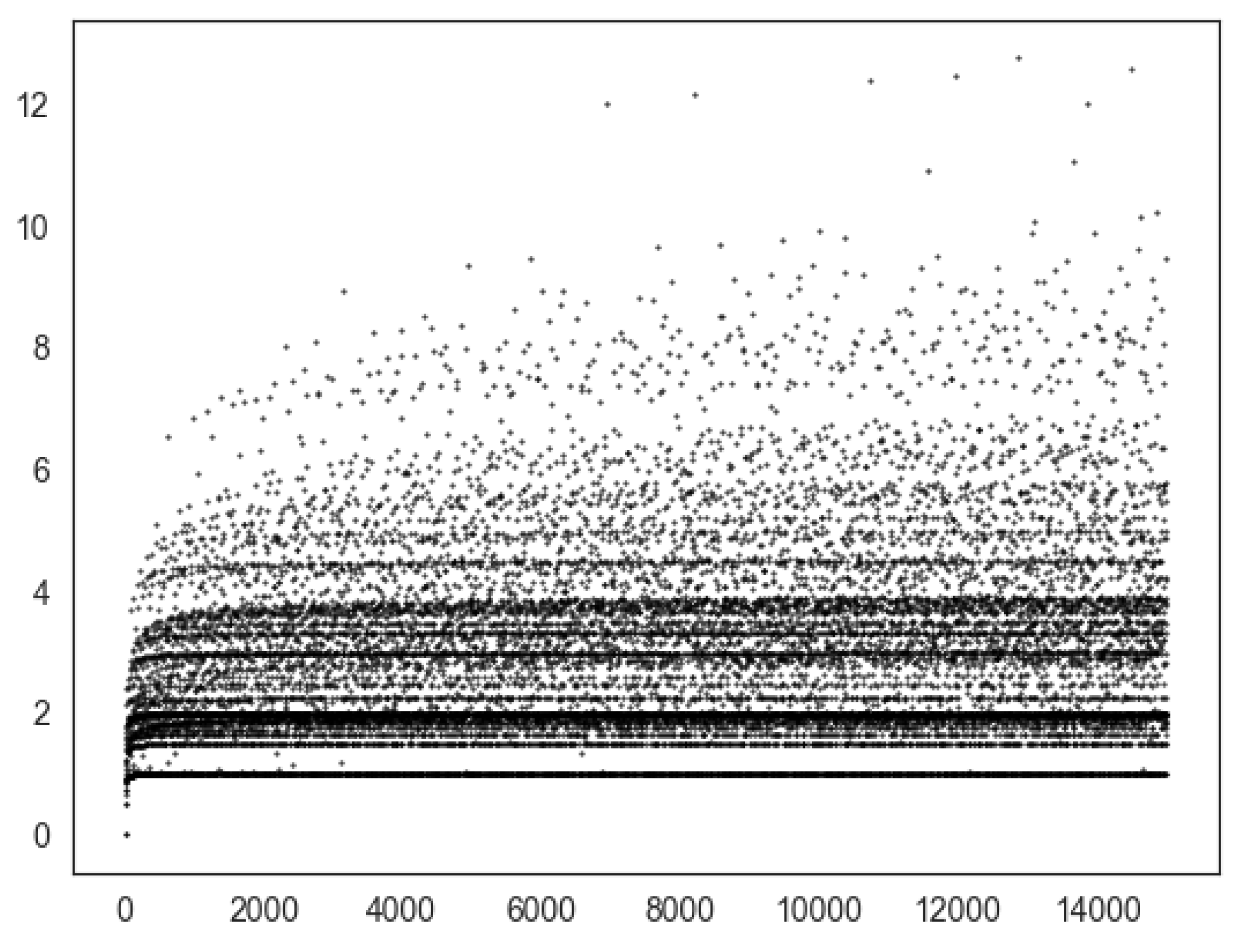
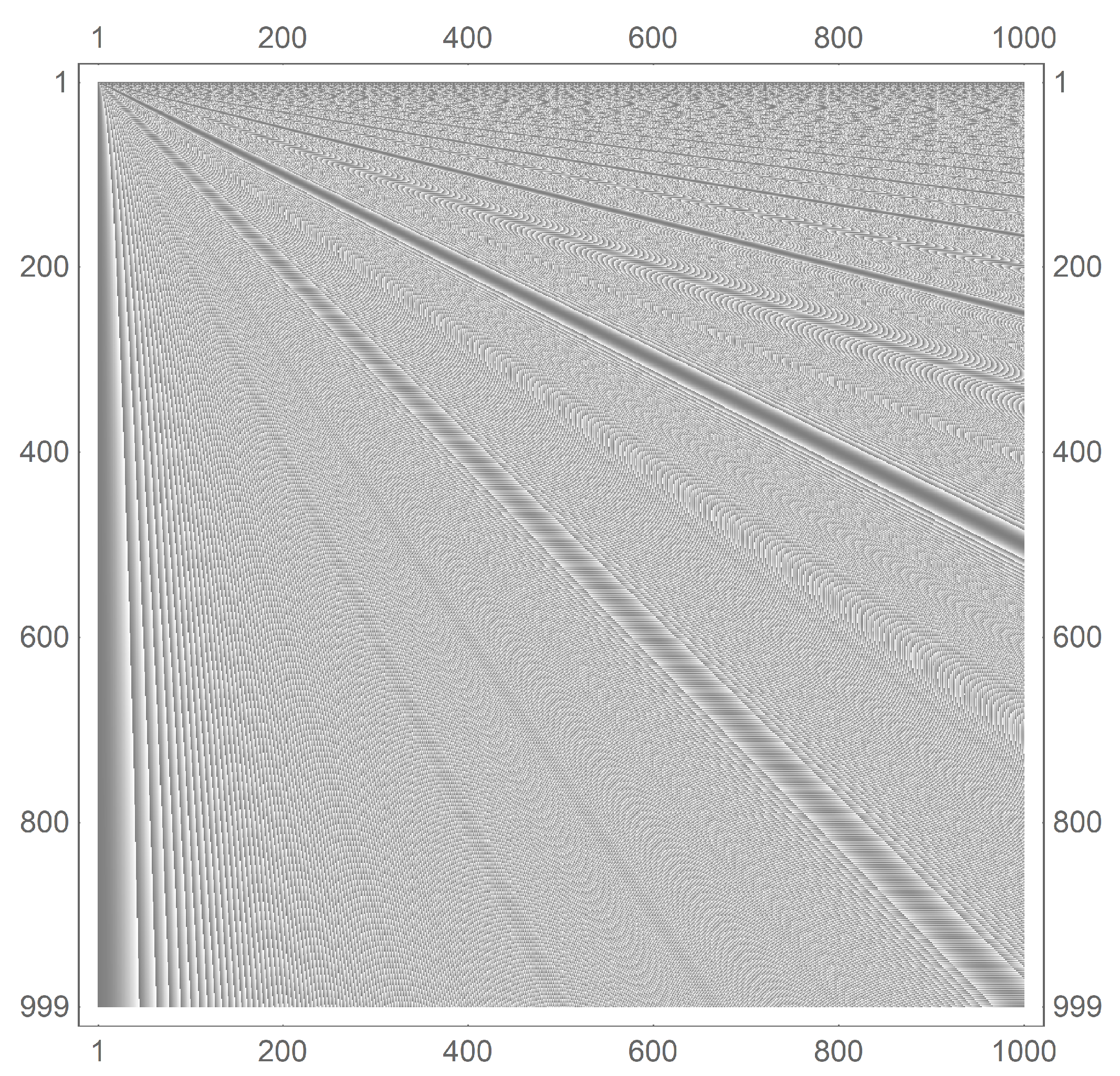
It is particularly enlightening to superimpose the partitioning of ${\mathcal{T}}_m$ into perfect squares and nonsquares onto the graph representations. Figure 6 shows this for the case of ${\mathcal{G}}_{15}$. Under modulo $m=15$, the perfect squares are 0, 1, 6, and 10 (indicated as red vertices), and 3 and 13 are nonsquares.

Returning to Figure 10 through Figure 12, the graph representation provides additional insight into the nature of the perfect square and nonsquare subsets. First, is it recognized that the ultimate vertex is sometimes a perfect square and sometimes a nonsquare according to the following conjecture.

Conjecture 7.

For $m=p$ where $p^2$ is an odd prime, then if $p=1mod8$ or $3mod8$, the ultimate vertex is a perfect square. Likewise, if $p=5mod8$ or $7mod8$, then the ultimate vertex is a nonsquare.

Additionally, the edges of the petals, i.e., $\frac{p-1}{2}$ and $\frac{p+1}{2}$ away from the ultimate vertex, are always nonsquares. This is a direct consequence of Theorem 11. Finally, one can state the following conjecture.

Conjecture 8.

Analogous vertices on the petals of $G_{p^2}$ graphs are of the same type: perfect square or nonsquare.

9. Self-Similarity

One method for generating the triangular numbers is to write out the positive integers starting with $k=1$ in rows of a table, where the first row contains only one column. Each subsequent row contains one additional column. It is obvious that the right-most entries in such a table will be the triangular numbers. One can now replace each integer in the table by its corresponding value modulo m. Then the rightmost entries are the triangle numbers’ moduli m. The three tables below are for $m=4$ (left), $m=5$ (middle), and $m=6$ (right).

$$\begin{array}{l} \begin{array}{c}1\\ 2& 3\\ 0& 1& 2\\ 3& 0& 1& 2\\ 3& 0& 1& 2& 3\\ 0& 1& 2& 3& 0& 1\\ 2& 3& 0& 1& 2& 3& 0\end{array}\\ \begin{array}{cccccccc}1& 2& 3& 0& 1& 2& 3& 0\\ 1& 2& 3& 0& 1& 2& 3& 0& 1\\ 2& 3& 0& 1& 2& 3& 0& 1& 2& 3\\ 0& 1& 2& 3& 0& 1& 2& 3& 0& 1& 2\\ 3& 0& 1& 2& 3& 0& 1& 2& 3& 0& 1& 2\\ 3& 0& 1& 2& 3& 0& 1& 2& 3& 0& 1& 2& 3\\ 0& 1& 2& 3& 0& 1& 2& 3& 0& 1& 2& 3& 0& 1\\ 2& 3& 0& 1& 2& 3& 0& 1& 2& 3& 0& 1& 2& 3& 0\\ 1& 2& 3& 0& 1& 2& 3& 0& 1& 2& 3& 0& 1& 2& 3& 0\end{array}\end{array}\begin{array}{l} \begin{array}{c}1\\ 2& 3\\ 4& 0& 1\\ 2& 3& 4& 0\\ 1& 2& 3& 4& 0\\ 1& 2& 3& 4& 0& 1\\ 2& 3& 4& 0& 1& 2& 3\\ 4& 0& 1& 2& 3& 4& 0& 1\\ 2& 3& 4& 0& 1& 2& 3& 4& 0\end{array}\\ \begin{array}{cccccccccc}1& 2& 3& 4& 0& 1& 2& 3& 4& 0\\ 1& 2& 3& 4& 0& 1& 2& 3& 4& 0& 1\\ 2& 3& 4& 0& 1& 2& 3& 4& 0& 1& 2& 3\\ 4& 0& 1& 2& 3& 4& 0& 1& 2& 3& 4& 0& 1\\ 2& 3& 4& 0& 1& 2& 3& 4& 0& 1& 2& 3& 4& 0\\ 1& 2& 3& 4& 0& 1& 2& 3& 4& 0& 1& 2& 3& 4& 0\\ 1& 2& 3& 4& 0& 1& 2& 3& 4& 0& 1& 2& 3& 4& 0& 1\end{array}\end{array}\begin{array}{l} \begin{array}{c}1\\ 2& 3\\ 4& 5& 0\\ 1& 2& 3& 4\\ 5& 0& 1& 2& 3\\ 4& 5& 0& 1& 2& 3\\ 4& 5& 0& 1& 2& 3& 4\\ 5& 0& 1& 2& 3& 4& 5& 0\\ 1& 2& 3& 4& 5& 0& 1& 2& 3\\ 4& 5& 0& 1& 2& 3& 4& 5& 0& 1\\ 2& 3& 4& 5& 0& 1& 2& 3& 4& 5& 0\end{array}\\ \begin{array}{cccccccccccc}1& 2& 3& 4& 5& 0& 1& 2& 3& 4& 5& 0\\ 1& 2& 3& 4& 5& 0& 1& 2& 3& 4& 5& 0& 1\\ 2& 3& 4& 5& 0& 1& 2& 3& 4& 5& 0& 1& 2& 3\\ 4& 5& 0& 1& 2& 3& 4& 5& 0& 1& 2& 3& 4& 5& 0\\ 1& 2& 3& 4& 5& 0& 1& 2& 3& 4& 5& 0& 1& 2& 3& 4\end{array}\end{array}$$

The vertical line in these tables demarks the first $2m$ cycle. The self-similarity of the triangular numbers modulo m is nicely exposed in this arrangement. One quickly notices that if the columns to the left of the vertical line are deleted, the resulting table is identical to the original.

Figure 14 is a visual representation of the self-similar nature of the triangular numbers’ moduli m. The graph shows the (grayscale normalized) $T\left(k\right)modm$ (horizontal dimension) versus m (vertical dimension). The dark band running from the origin to the point (1000, 500) is the manifestation of the terminal zeros in each cycle. The alternating dark/light band running along the 45 degree line is a manifestation of the odd (zero) and even ($\frac{m}{2}$) value at the mid-point of the cycle.

The repeated pattern appears in the upper-right portion of the graph. One sees a scaling of the visual features seen in the lower-left portion of the graph.

10. Scaling Properties

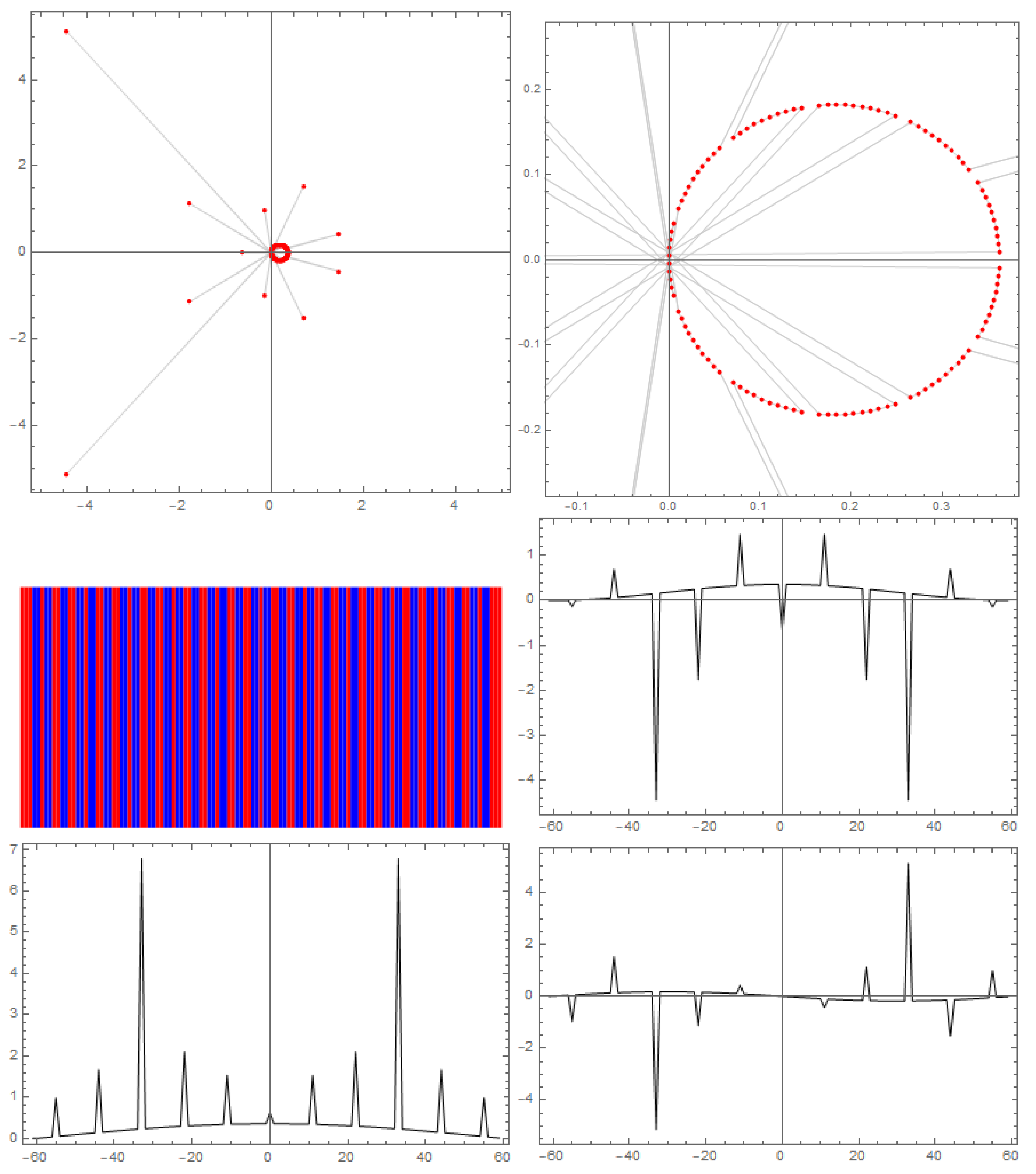
The graphical representation of m being a prime power clearly exposes a scaling feature for ${\mathcal{T}}_{p^n}⟷{\mathcal{T}}_{p^{n+2}}$ This will be explored in this section.

10.1. Sprays

The concept of a spray is introduced to aid the study of the scaling properties of the ${\mathcal{T}}_m$ graphs.

Definition 8.

Spray. A set of simple linear paths between two primary vertices. The distinct paths are otherwise identical. That is, they have the same numbers of intermediate vertices and edges, and the degree of the intermediate vertices is exactly two. The paths of a first order spray do not share a vertex. A second-order spray can be thought of as a spray of first order sprays; jth order sprays are sprays of $(j-1)$th order sprays.

Figure 11 shows an example of sprays as seen in the ${\mathcal{G}}_{5^3}$ and ${\mathcal{G}}_{5^4}$ graphs. In these cases, one sees that between each primary vertex there are five distinct linear paths, and in each path there are four intermediate second degree vertices. The examples of ${\mathcal{G}}_{5^5}$ and ${\mathcal{G}}_{5^6}$ show second order sprays, as one sees five sprays emerging from either the ultimate or penultimate vertices. The first order sprays occur between adjacent antepenultimate vertices (and also between an antepenultimate vertex and either an ultimate or penultimate vertex). These feature generalize for all odd primes. The above analysis continues for ${\mathcal{G}}_{p^{2n-1}}$ and ${\mathcal{G}}_{p^{2n}}$ in the obvious way.

10.2. Sprays, Renormalization, and Fractal Character

A natural renormalization scheme is provided by the sprays for prime power graphs. If the first order sprays in ${\mathcal{G}}_{p^n}$ are replaced by edges, the graph reduces to ${\mathcal{G}}_{p^{n-2}}$. In this process, second-order sprays become first order sprays. Likewise, kth order sprays become $(k-1)$th order sprays. This process can be repeated until ${\mathcal{G}}_{p^n}$ is fully reduced to ${\mathcal{G}}_p$ when k is odd and ${\mathcal{G}}_{p^2}$ when k is even.

The reverse of the renormalization scheme can be performed to scale up a graph from base graphs ${\mathcal{G}}_p$ and ${\mathcal{G}}_{p^2}$. In this case, each edge is replaced with a spray of p paths; each path has p edges. In a certain sense, this “fractalizes” the graph in that each edge is blown up into a spray indefinitely. As an example, one can consider the scale up from ${\mathcal{G}}_{5^2}$ to ${\mathcal{G}}_{5^4}$ to ${\mathcal{G}}_{5^6}$ seen going down the left side of Figure 11. The ultimate vertex in ${\mathcal{G}}_{5^2}$ has five edges emerging from it. These become five groups of five or $5^2$ edges in ${\mathcal{G}}_{5^4}$ and $5^3$ edges in ${\mathcal{G}}_{5^6}$. The other vertices behave similarly. Thus, the act of raising the power on the prime is akin to zooming in on a fractal object.

Some characteristics of the graphs of prime powers can be immediately gleaned from their scaling structures. This leads to two conjectures regarding the graph’s diameter and radius.

Conjecture 9.

The graph diameter,

$$d\left({\mathcal{G}}_{p^n}\right)=\left\{\begin{array}{cc}{p}^{\frac{n}{2}}-1\hfill & if n even\hfill \\ \frac{p^{\frac{n+1}{2}}-1}{2}\hfill & if n odd.\hfill \end{array}\right.$$

Conjecture 10.

The graph radius $r\left({\mathcal{G}}_{p^n}\right)=\frac{d\left({\mathcal{G}}_{p^n}\right)}{2}$. This does not hold when n is odd and $p=3$.

Specific to the even prime powers case, in which the broad scale flower structure is maintained upon scaling, two definitions related to diameter and radius are useful. In those cases, there is a single ultimate vertex. We then define the following.

Definition 9.

Ultimate distance, u. The distance from a vertex from the ultimate vertex.

Definition 10.

Ultimate radius $u_r$. The maximum distance from the ultimate vertex for a graph.

Consideration of these definitions leads to the following conjecture.

Conjecture 11.

The ultimate radius and the graph radius are related as$u_r\left({\mathcal{G}}_{p^n}\right)=r\left({\mathcal{G}}_{p^n}\right)$.

11. Application to Harmonic Analysis

An interesting application of the triangular numbers mod m is the consideration of the lacunary trigonometric function defined on the unit circle in the complex plane, where $\tau \equiv e^{i\varphi }$ [17,18].

$$f\left(z\right)=\sum _{k=0}^{\infty }{\tau }^{T\left(k\right)}.$$

Associated with such a function is the sequence of partial summations, $\mathcal{F}\equiv \left\{f^N\right\}$, where $N\in \mathbb{N}$ and

$$f^{\left(N\right)}\left(z\right)=\sum _{k=0}^N{\tau }^{T\left(k\right)}.$$

The special cases of $\tau =e^{\frac{i\pi }{n}}$ give rise to an interesting family of functions. Here,

$$f_n\left(e^{\frac{i\pi }{n}}\right)=\sum _{k=0}^{\infty }{\left(e^{\frac{i\pi }{n}}\right)}^{T\left(k\right)}=\sum _{k=0}^{\infty }{e}^{\frac{i\pi T\left(k\right)}{n}}.$$

The triangular lacunary trigonometric function can be written as a Jacobi theta function (see [19], chapter 16). Writing

$$f_n=\sum _{k=0}^{\infty }{e}^{\frac{i\pi q}{2n}\left(k^2+k\right)}.$$

Completing the square in the exponent, extending the dummy index to $-\infty$, and dividing by two yields

$$f_n=\frac{1}{2}{e}^{\frac{i\pi q}{8n}}\sum _{k=-\infty }^{\infty }{e}^{\frac{i\pi q}{2n}{\left(k+\frac{1}{2}\right)}^2},$$

where the summation is recognized at the second Jacobi theta function (see [19], chapter 16),

$$f_n=\frac{1}{2}{e}^{\frac{i\pi q}{8n}}{\vartheta }_2\left(0,e^{\frac{i\pi q}{2n}}\right).$$

While the above relation is helpful in putting these triangular lacunary trigonometric systems in a larger mathematical context, it is as interesting to study the sequence of partial summations associated with the lacunary function. The Nth member of the associated finite summation is

$$f_n^{\left(N\right)}\left(e^{\frac{i\pi }{n}}\right)=\sum _{k=0}^N{e}^{\frac{i\pi T\left(k\right)}{n}}.$$

The $2\pi$ periodic nature of $e^{i\varphi }$ gives rise to $T\left(k\right)mod2n$. Thus, the machinery of the above theorems can be brought to bear on these functions.

A consequence of Theorem 1 suggests the sequence of finite sums of a given n has $4n$-cycles (bounded but not convergent). This suggests that a useful representation of $f_n$ is a $4n$ member sequence that consists of one cycle.

Definition 11.

$4n$-cycle representation. The $4n$-cycle representation of $f_n$ is denoted by ${\mathcal{F}}_n$. The auxiliary set of individual terms, $e^{\frac{i\pi T\left(k\right)}{n}}$, is denoted by ${\mathcal{E}}_n.$

As a first example, consider $f_1$:

$$f_1^{\left(N\right)}\left(e^{i\pi }\right)=\sum _{k=0}^N{e}^{i\pi T\left(k\right)}.$$

It is immediately clear that one need only consider ${\mathcal{T}}_2=\left\{1,0,1,0\right\}$ to determine that ${\mathcal{F}}_n=\left\{1,0,-1,0\right\}$. $f_1$ itself is the infinite summation, $f_1=1+0-1+0+1+0-1\dots$.

As a second example, consider $f_4$. Here ${\mathcal{T}}_4=\left\{0,1,3,2,2,3,1,0\right\}$ leads to ${\mathcal{F}}_2=\left\{1,1+i,1,0,-1,-1-i,-1,0\right\}$.

While not convergent, one can see that the $f_n$ are Cesàro summable and Cesàro converge to zero (see [20], page 96).

A lemma and a theorem regarding $f_n$ follow quickly from the theorems in the above sections.

Lemma 4.

The jth element of ${\mathcal{E}}_n$ has its additive inverse at the $2n+j$th element of ${\mathcal{E}}_n$$0\le j\le 2n$.

Proof. 

Given that the jth element of ${\mathcal{E}}_n$ is $e^{i\frac{\pi T\left(j\right)}{n}}$, the $2n+j$th element is $e^{i\frac{\pi T(2n+j)}{n}}$. Expanding and simplifying the expression leaves one with $-e^{i\frac{\pi T\left(j\right)}{n}}$. This is the additive inverse of the jth term. □

Theorem 21.

The sum of the elements of ${\mathcal{F}}_n$ is zero.

Proof. 

From Lemma 4, one notices that each term j in ${\mathcal{E}}_n$ will have its additive inverse at the $(2n+j)$th term. From Theorem 1, one also recognizes the $(2n+j)$th term =$(2n-j)$th term. Remembering that ${\mathcal{F}}_n$ is a 4n cycle, it is clear to see that the sum of ${\mathcal{F}}_n$ will be zero at the $2n$th term. Therefore, the jth term will have its additive inverse at the $(2n+j)$th term. This leads to the summation of all the elements of ${\mathcal{F}}_n$ being zero. □

Interestingly, this is related to the theory of Gaussian summations [21,22,23].

12. Conclusions

This work focused on the structure and properties of the triangular numbers modulo m. The most important aspect of the structure of these numbers is their periodic nature. It was proven that the triangular numbers’ moduli m form a $2m$-cycle for any m. Additional structural features and properties of this system were presented and discussed. This discussion was aided by various representations of these sequences, such as graphs and through discrete Fourier transformation. The concept of saturation was developed and explored, as were monoid sets and the roles of perfect squares and nonsquares. The triangular numbers’ moduli m have self-similarity and scaling features which were briefly discussed as well. It is hoped that this work serves to collect some of the characteristics of the important case of triangular number modulo m.

The story of the triangular number modulo m is far from complete. The numerous conjectures are awaiting proof. Direct numerical analysis and network analysis are certain to provide deeper insight than was presented here. A suggestion from an anonymous reviewer was, “Since the triangular numbers are by definition from all distinct drawings of subsets, a set algorithms refining random generators for order statistics may benefit from the series of triangular numbers modulo m”. An potential example here is the Mersenne Twister generator [24,25]. Finally, models of physical phenomena could potentially be found.

References

1. Deza, E.; Deza, M.-M. Figurate Numbers; World Scientific: Hackensack, NJ, USA, 2012. [Google Scholar]
2. Hoggatt, V.E., Jr.; Bicknell, M. Triangular numbers. Fibonacci Q. 1974, 12, 221–230. [Google Scholar]
3. Ono, K.; Robbins, S.; Wahl, P.T. On the representation of integers as sums of triangular numbers. Aequationes Math. 1995, 50, 73–94. [Google Scholar] [CrossRef]
4. Schroeder, M.R. Number Theory in Science and Communication; Springer: Berlin/Heidelberg, Germany, 1984. [Google Scholar]
5. Sun, Z.-W. On sums of primes and triangular numbers. J. Comb. Number Theory 2009, 1, 65–76. [Google Scholar]
6. Wall, D.D. Fibonacci Series Modulo m. Am. Math. Mon. 1960, 67, 525–532. [Google Scholar] [CrossRef]
7. Özkan, E.; Aydin, H.; Dikici, R. 3-Step Fibonacci series modulo m. Appl. Math. Comput. 2003, 143, 165–172. [Google Scholar] [CrossRef]
8. Aydin, H.; Dikici, R.; Smith, G.C. Wall and Vinson Revisited. In Applications of Fibonacci Numbers; Bergum, G.E., Philippou, A.N., Horadam, A.F., Eds.; Springer: Dordrecht, The Netherlands, 1993. [Google Scholar]
9. Dikici, R.; Özkan, E. An application of Fibonacci sequences in groups. Appl. Math. Comput. 2003, 136, 323–331. [Google Scholar] [CrossRef]
10. Slone, N.J.A. Online Encyclopedia on Integer Sequences. Available online: https://oeis.org/ (accessed on 28 May 2022).
11. Jusdon, T.W. Absract Algebra; PWS Publishing Company: Boston, MA, USA, 1994. [Google Scholar]
12. Fraleigh, J.B. A First Course in Abstract Algebra, 4th ed.; Addison-Wesley: Reading, MA, USA, 1989. [Google Scholar]
13. Andrews, G.E. Number Theory; Dover Publications: New York, NY, USA, 1971. [Google Scholar]
14. Papoulis, A. Probability, Random Variables, and Stochastic Processes; McGraw-Hill: New York, NY, USA, 1984. [Google Scholar]
15. Newman, M.E.J. The structure and function of complex networks. SIAM Rev. 2003, 45, 167–256. [Google Scholar] [CrossRef] [Green Version]
16. Aigner, M. A Course in Enumeration; Springer: Berlin/Heidelberg, Germany, 2007. [Google Scholar]
17. Coutsias, E.A.; Kazarinoff, N.D. Disorder, renormalizability, theta functions and Cornu spirals. Phys. D Nonlinear Phenom. 1987, 26, 295–310. [Google Scholar] [CrossRef]
18. Vogt, T.; Ulness, D.J. Cornu spirals and the triangular lacunary trigonometric system. Fractal Fract. 2019, 3, 40. [Google Scholar] [CrossRef] [Green Version]
19. Abramowitz, M.; Stegun, I.A. Handbook of Mathematical Functions; Dover Publications: New York, NY, USA, 1972. [Google Scholar]
20. Hardy, G.H. Divergent Series; AMS Chelsea Publishing: New York, NY, USA, 1991. [Google Scholar]
21. Lehmer, D.H. Incomplete Gauss sums. Mathematika 1976, 23, 125–135. [Google Scholar] [CrossRef]
22. Paris, R.B. An asymptotic approximation for incomplete Gauss sums. J. Comput. Appl. Math. 2008, 212, 16–30. [Google Scholar] [CrossRef] [Green Version]
23. Berry, M.V.; Goldberg, J. Renormalization of curlicues. Nonlinearity 1988, 1, 1–26. [Google Scholar] [CrossRef]
24. Matsumoto, M.; Nishimura, T. Mersenne twister: A 623-dimensionally equidistributed uniform pseudo-random number generator. ACM Trans. Model. Comput. Simul. 1998, 8, 3–30. [Google Scholar] [CrossRef] [Green Version]
25. Jäntschi, L. Detecting Extreme Values with Order Statistics in Samples from Continuous Distributions. Mathematics 2020, 8, 216. [Google Scholar] [CrossRef] [Green Version]
Figure 1. Schematic of the various sets discussed in this work and their relationships. Top row: Lossless compression of information about the sequence of triangular numbers modulo m based on Theorems 1–3. Second row: Application of Theorem 4. Note for odd values of m, this information compression is lossless. It is lossy, however, when m is even. Bottom row: Mapping of the ordered sequences in S m to the unordered sets. As the order is lost, these maps are lossy. Data compression is dependent on the specific value of m. This data compression finally results in the representation of the sequence of triangular numbers modulo m as saturation, 0 s 1 via Definition 5.
Appliedmath 02 00020 g001
Figure 2. Saturation, s, (ordinate) versus m (abscissa) for the first 700,000 integers m. The top graph shows all the data, and the bottom graph shows a blow-up of the low saturation values. As will be seen to be typical throughout this work, there are striation patterns in the graph. The (rare) points that fall below the main region of values are highly composite numbers.
Appliedmath 02 00020 g002
Figure 3. Plot of M r (ordinate) versus m (abscissa) up to m = 15,000. The points at M r = 1 are m values of the form 2 a 3 b for all nonnegative integers, a and b = 1 or 2, as per Theorem 19.
Appliedmath 02 00020 g003
Figure 4. Plot of R (ordinate) for m (abscissa) up to 15,000. More often than not, the nonsquare excess is below one. There also appear to be striations of high concentrations of particular values of R. Finally, R appears to be bounded between roughly 0.3 and 2.2 as m gets large.
Appliedmath 02 00020 g004
Figure 5. Plot of R (ordinate) for m = p primes for 5 to 1223 (abscissa). The color represents set of primes of the form 8 n + 1 (red), 8 n + 3 (green), 8 n + 5 (orange), and 8 n + 7 (blue). Inset: a blow-up of the ordinate. The colored curves are the functions R = p p + 2 (red), R = p p + 6 (green), and R = p p 2 (blue). Inset: The relative percent error of the model function compared to the data.
Appliedmath 02 00020 g005
Figure 6. The example of a graph construction from T 15 for the case of m = 15 . The top sequence of numbers is T 15 . By Theorem 1, this reduces to the sequence of red and blue numbers on the second line. The red numbers indicate the perfect squares for m = 15 and the blue represent the nonsquares. The right pointing arrow indicates the further reduction to the set of unique triangular numbers modulo 15. The sequence can then be represented by the block graph of red and blue segments, or as a (network) graph (called G 15 ). This is discussed in Section 8.3. The set of unique triangular numbers modulo 15 is the set of vertices (identified with solid gray arrows), and the pathway through the sequence is the set of edges (identified with dashed gray arrows). Red vertices (edges) indicate perfect squares (a connection between a pair of perfect squares). It is the same for blue but for nonsquares. The purple edges indicate a connection between a perfect square and a nonsquare.
Appliedmath 02 00020 g006
Figure 7. Fourier analysis of the perfect square and nonsquare profiles for the case of m = 17,389 (the 2000th) prime. The top panels show the scatter plot of the discrete Fourier transform of T 17,389 (full plot, left panel, zoomed in, right panel). The ordinate is the imaginary value, and the abscissa is the real value. The middle left panel shows the block-color plot of the perfect squares (red) and nonsquares (blue) in T 17,389 . The bottom left panel shows the absolute value of the discrete Fourier transform. The middle and bottom right panels show the real and imaginary parts of the the discrete Fourier transform, respectively. Fourier transforms were performed using Mathematica.
Appliedmath 02 00020 g007
Figure 8. Fourier analysis of the perfect square and nonsquare profiles for the case of m = 11 2 = 121 . The top panels show the scatter plot of the discrete Fourier transform of T 121 (full plot, left panel, zoomed in, right panel.) The ordinate is the imaginary value and the abscissa is the real value. The middle left panel shows the block-color plot of the perfect squares (red) and nonsquares (blue) in T 121 . The bottom left panel shows the absolute value of the discrete Fourier transform. The middle right and bottom right panels show the real and imaginary parts of the discrete Fourier transform, respectively. Fourier transforms were performed using Mathematica.
Appliedmath 02 00020 g008
Figure 9. Further investigation of the structure of the discrete Fourier transform for the cases of m as primes squared for the primes from 3 to 31. The circles of radius 2 p are fits centered at z = 2 p . One notes that p sets of p 1 points are symmetrically arranged around the circles.
Appliedmath 02 00020 g009
Figure 10. Several examples of graph representations of T m . All powers of two are linear path graphs of size m. Likewise, all primes are linear path graphs of size m + 1 2 . Prime squares are “flower” graphs with m 1 2 petals and one stem. The stem has m 1 2 vertices made up of m 1 vertices. Finally, there is one central vertex called the ultimate vertex which is of degree m. The base of the stem is of degree one; all remaining vertices are of degree two. The graphs are colored according to whether a vertex represents a perfect square (red) or a nonsquare (blue).
Appliedmath 02 00020 g010
Figure 11. Examples of graphs for prime powers, m = 5 a for a ranging from 2 through 6 are shown. The even powers maintain the general shape of the flower graph. The scaling procedure is described in Section 10. The odd powers maintain the general shape of the linear path for the base prime (again, scaling is described in the text). The vertices are referred to using the ultimate, penultimate, and antepenultimate vernacular. For the case of m = p 4 , there is one ultimate vertex of degree p 2 and each petal has p 1 penultimate vertices. For the case of m = p 6 , there is one ultimate vertex of degree p 4 , and each petal has p 1 penultimate vertices; between each penultimate vertices there are p 1 antepenultimate vertices (too small to see in the figure). The odd powers proceed in a similar manner. The graphs are colored according to whether a vertex represents a perfect square (red) or a nonsquare (blue).
Appliedmath 02 00020 g011
Figure 12. Examples of graphs in which m is composite. The top graph shows the case for m = 3 × 5 × 7 × 11 × 13 = 15,015. High composites get rather complicated, but one can still see a web-like overall structure which is the nature of double composites (two distinct primes). The lower graphs show three examples. In cases where both primes are odd, there is one vertex of degree one; otherwise, the nodes are of degree four (interior of the web) or two (edge of the web). Additionally, on graphs for all products of two odd primes there are p 1 1 2 · p 2 1 2 internal faces. There is always exactly one triangle. The remaining internal faces are four-sided quadrilaterals. The graphs are colored according to whether a vertex represents a perfect square (red) or a nonsquare (blue).
Appliedmath 02 00020 g012
Figure 13. Plot of | E | | V | (ordinate) for m up to 15,000 (abscissa). Here too, the scatter plot shows striations. While there is a preponderance of ratios that are greater than 1, graphs for m = 2 n and m = p , where p is prime have a ratio that goes to 1 for large m.
Appliedmath 02 00020 g013
Figure 14. Visual representation of the structure of the triangular numbers modulo m for 0 m < 1000 . The vertical axis is the m value and the horizontal axis is the value of T ( k ) mod m . The scaling structure is seen quite clearly as the eye sweeps from the lower-left corner to the upper-right corner of the plot. Gray represents low values and white represents high values (values normalized by 1 / m to show better contrast).
Appliedmath 02 00020 g014
Publisher’s Note: MDPI stays neutral with regard to jurisdictional claims in published maps and institutional affiliations.