Article

Local Normal Approximations and Probability Metric Bounds for the Matrix-Variate T Distribution and Its Application to Hotelling’s T Statistic

by
Frédéric Ouimet
1,2
1
Department of Mathematics and Statistics, McGill University, Montreal, QC H3A 0B9, Canada
2
Division of Physics, Mathematics and Astronomy, California Institute of Technology, Pasadena, CA 91125, USA
AppliedMath 2022, 2(3), 446-456; https://doi.org/10.3390/appliedmath2030025
Submission received: 22 June 2022 / Revised: 18 July 2022 / Accepted: 21 July 2022 / Published: 1 August 2022

Abstract

:
In this paper, we develop local expansions for the ratio of the centered matrix-variate T density to the centered matrix-variate normal density with the same covariances. The approximations are used to derive upper bounds on several probability metrics (such as the total variation and Hellinger distance) between the corresponding induced measures. This work extends some previous results for the univariate Student distribution to the matrix-variate setting.

1. Introduction

For any n N , define the space of (real symmetric) positive definite matrices of size n × n as follows:
S + + n : = M R n × n : M is symmetric and positive definite .
For d , m N , ν > 0 , M R d × m , Σ S + + d and Ω S + + m , the density function of the centered (and normalized) matrix-variate T distribution, hereafter denoted by T d , m ( ν , Σ , Ω ) , is defined, for all X R d × m , by
K ν , Σ , Ω ( X ) : = Γ d ( 1 2 ( ν + m + d 1 ) ) Γ d ( 1 2 ( ν + d 1 ) ) | I d + ν 1 Σ 1 X Ω 1 X | ( ν + m + d 1 ) / 2 ( ν π ) m d / 2 | Σ | m / 2 | Ω | d / 2 ,
(see, e.g., (Definition 4.2.1 in [1])) where ν is the number of degrees of freedom, and
Γ d ( z ) = S S + + d | S | z ( d + 1 ) / 2 exp ( tr ( S ) ) d S = π d ( d 1 ) / 4 j = 1 d Γ z j 1 2 , ( z ) > d 1 2 ,
denotes the multivariate gamma function—see, e.g., (Section 35.3 in [2]) and [3]—and
Γ ( z ) = 0 t z 1 e t d t , ( z ) > 0 ,
is the classical gamma function. The mean and covariance matrix for the vectorization of T T d , m ( ν , Σ , Ω ) , namely
vec ( T ) : = ( T 11 , T 21 , , T d 1 , T 12 , T 22 , , T d 2 , , T 1 m , T 2 m , , T d m ) ,
( vec ( · ) is the operator that stacks the columns of a matrix on top of each other) are known to be (see, e.g., Theorem 4.3.1 in [1], but be careful of the normalization):
E [ vec ( T ) ] = 0 d m ( i . e . , E [ T ] = 0 d × m ) ,
and
V ar ( vec ( T ) ) = ν ( ν 2 ) Σ Ω , ν > 2 .
The first goal of our paper (Theorem 1) is to establish an asymptotic expansion for the ratio of the centered matrix-variate T density (1) to the centered matrix-variate normal (MN) density with the same covariances. According to (Gupta and Nagar [1], Theorem 2.2.1), the density of the MN d , m ( 0 d × m , Σ Ω ) distribution is
g Σ , Ω ( X ) = exp 1 2 tr Σ 1 X Ω 1 X ( 2 π ) m d / 2 | Σ | m / 2 | Ω | d / 2 , X R d × m .
The second goal of our paper (Theorem 2) is to apply the log-ratio expansion from Theorem 1 to derive upper bounds on multiple probability metrics between the measures induced by the centered matrix-variate T distribution and the corresponding centered matrix-variate normal distribution. In the special case m = 1 , this gives us probability metric upper bounds between the measure induced by Hotelling’s T statistic and the associated matrix-normal measure.
To give some practical motivations for the MN distribution (2), note that noise in the estimate of individual voxels of diffusion tensor magnetic resonance imaging (DT-MRI) data has been shown to be well modeled by a symmetric form of the MN 3 × 3 distribution in [4,5,6]. The symmetric MN voxel distributions were combined into a tensor-variate normal distribution in [7,8], which could help to predict how the whole image (not just individual voxels) changes when shearing and dilation operations are applied in image wearing and registration problems; see Alexander et al. [9]. In [10], maximum likelihood estimators and likelihood ratio tests are developed for the eigenvalues and eigenvectors of a form of the symmetric MN distribution with an orthogonally invariant covariance structure, both in one-sample problems (for example, in image interpolation) and two-sample problems (when comparing images) and under a broad variety of assumptions. This work extended significantly the previous results of Mallows [11]. In [10], it is also mentioned that the polarization pattern of cosmic microwave background (CMB) radiation measurements can be represented by 2 × 2 positive definite matrices; see the primer by Hu and White [12]. In a very recent and interesting paper, Vafaei Sadr and Movahed [13] presented evidence for the Gaussianity of the local extrema of CMB maps. We can also mention [14], where finite mixtures of skewed MN distributions were applied to an image recognition problem.
In general, we know that the Gaussian distribution is an attractor for sums of i.i.d. random variables with finite variance, which makes many estimators in statistics asymptotically normal. Similarly, we expect the MN distribution (2) to be an attractor for sums of i.i.d. random matrices with finite variances (Hotelling’s T-squared statistic is the most natural example), thus including many estimators, such as sample covariance matrices and score statistics for matrix parameters. In particular, if a given statistic or estimator is a function of the components of a sample covariance matrix for i.i.d. observations coming from a multivariate Gaussian population, then we could study its large sample properties (such as its moments) using Theorem 1 (for example, by turning a Student-moments estimation problem into a Gaussian-moments estimation problem).
The following is a brief outline of the paper. Our main results are stated in Section 2 and proven in Section 3. Technical moment calculations are gathered in Appendix A.
Notation 1.
Throughout the paper, a = O ( b ) means that lim sup | a / b | < C as ν , where C > 0 is a universal constant. Whenever C might depend on some parameter, we add a subscript (for example, a = O d ( b ) ). Similarly, a = o ( b ) means that lim | a / b | = 0 , and subscripts indicate which parameters the convergence rate can depend on. If a = ( 1 + o ( 1 ) ) b , then we write a b . The notation tr ( · ) will denote the trace operator for matrices and | · | their determinant. For a matrix M R d × d that is diagonalizable, λ 1 ( M ) λ d ( M ) will denote its eigenvalues, and we let λ ( M ) : = ( λ 1 ( M ) , , λ d ( M ) ) .

2. Main Results

In Theorem 1 below, we prove an asymptotic expansion for the ratio of the centered matrix-variate T density to the centered matrix-variate normal (MN) density with the same covariances. The case d = m = 1 was proven recently in [15] (see also [16] for an earlier rougher version). The result extends significantly the convergence in distribution result from Theorem 4.3.4 in [1].
Theorem 1.
Let d , m N , Σ S + + d and Ω S + + m be given. Pick any η ( 0 , 1 ) and let
B ν , Σ , Ω ( η ) : = X R d × m : max 1 j d δ λ j ν 2 η ν 1 / 4
denote the bulk of the centered matrix-variate T distribution, where
Δ X = Σ 1 / 2 X Ω 1 / 2 and δ λ j : = ν 2 ν λ j ( Δ X Δ X ) , 1 j d .
Then, as ν and uniformly for X B ν , Σ , Ω ( η ) , we have
log [ ν / ( ν 2 ) ] m d / 2 K ν , Σ , Ω ( X ) g Σ , Ω ( X / ν / ( ν 2 ) ) = ν 1 1 4 tr ( Δ X Δ X ) 2 ( m + d + 1 ) 2 tr Δ X Δ X + m d ( m + d + 1 ) 4 + ν 2 1 6 tr ( Δ X Δ X ) 3 + ( m + d 1 ) 4 tr ( Δ X Δ X ) 2 + m d 24 ( 13 2 d 2 3 d ( 3 + m ) + 9 m 2 m 2 ) + ν 3 1 8 tr ( Δ X Δ X ) 4 ( m + d 1 ) 6 tr ( Δ X Δ X ) 3 + m d 24 26 + d 3 + 2 d 2 ( 3 + m ) + 11 m 6 m 2 + m 3 + d ( 11 9 m + 2 m 2 ) + O d , m , η 1 + tr ( Δ X Δ X ) 5 ν 4 .
Local approximations such as the one in Theorem 1 can be found for the Poisson, binomial and negative binomial distributions in [17] (based on Fourier analysis results from [18]), and [19] for the binomial distribution. Another approach, using Stein’s method, is used to study the variance-gamma distribution in [20]. Moreover, Kolmogorov and Wasserstein distance bounds are derived in [21,22] for the Laplace and variance-gamma distributions.
Below, we provide numerical evidence (displayed graphically) for the validity of the expansion in Theorem 1 when d = m = 2 . We compare three levels of approximation for various choices of S . For any given S S + + d , define
E 0 : = sup X B ν , Σ , Ω ( ν 1 / 4 ) log [ ν / ( ν 2 ) ] m d / 2 K ν , Σ , Ω ( X ) g Σ , Ω ( X / ν / ( ν 2 ) ) , E 1 : = sup X B ν , Σ , Ω ( ν 1 / 4 ) log [ ν / ( ν 2 ) ] m d / 2 K ν , Σ , Ω ( X ) g Σ , Ω ( X / ν / ( ν 2 ) ) ν 1 1 4 tr ( Δ X Δ X ) 2 ( m + d + 1 ) 2 tr Δ X Δ X + m d ( m + d + 1 ) 4 ,
E 2 : = sup X B ν , Σ , Ω ( ν 1 / 4 ) log [ ν / ( ν 2 ) ] m d / 2 K ν , Σ , Ω ( X ) g Σ , Ω ( X / ν / ( ν 2 ) ) ν 1 1 4 tr ( Δ X Δ X ) 2 ( m + d + 1 ) 2 tr Δ X Δ X + m d ( m + d + 1 ) 4 ν 2 1 6 tr ( Δ X Δ X ) 3 + ( m + d 1 ) 4 tr ( Δ X Δ X ) 2 + m d 24 ( 13 2 d 2 3 d ( 3 + m ) + 9 m 2 m 2 ) .
In the R software [23], we use Equation (7) to evaluate the log-ratios inside E 0 , E 1 and E 2 .
Note that X B ν , Σ , Ω ( ν 1 / 4 ) implies | tr ( ( Δ X Δ X ) k ) | d for all k N , so we expect from Theorem 1 that the maximum errors above ( E 0 , E 1 and E 2 ) will have the asymptotic behavior
E i = O d ( ν ( 1 + i ) ) , for all i { 0 , 1 , 2 } ,
or, equivalently,
lim inf ν log E i log ( ν 1 ) 1 + i , for all i { 0 , 1 , 2 } .
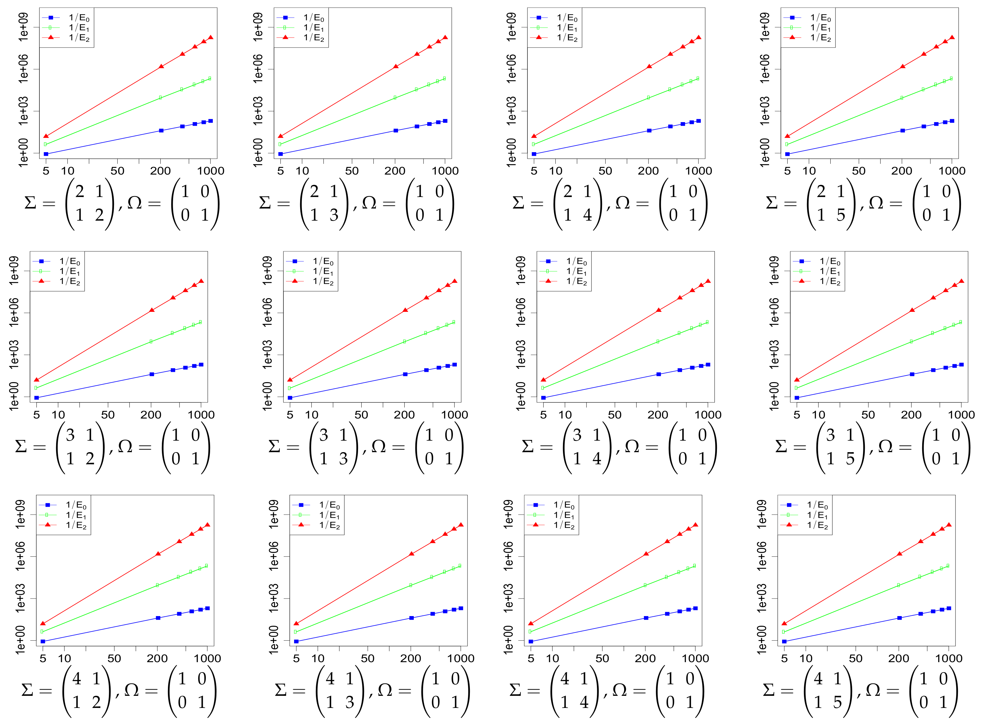
The property (5) is verified in Figure 1 below, for Ω = I 2 and various choices of Σ 2 × 2 . Similarly, the corresponding log-log plots of the errors as a function of ν are displayed in Figure 2. The simulations are limited to the range 5 ν 1005 . The R code that generated Figure 1 and Figure 2 can be found at Supplementary Material.
As a consequence of the previous theorem, we can derive asymptotic upper bounds on several probability metrics between the probability measures induced by the centered matrix-variate T distribution (1) and the corresponding centered matrix-variate normal distribution (2). The distance between Hotelling’s T statistic [24] and the corresponding matrix-variate normal distribution is obtained in the special case m = 1 .
Theorem 2
(Probability metric upper bounds). Let d , m N , Σ S + + d and Ω S + + m be given. Assume that X T d , m ( ν , Σ , Ω ) , Y MN d , m ( 0 d × m , Σ Ω ) , and let P ν , Σ , Ω and Q Σ , Ω be the laws of X and Y ν / ( ν 2 ) , respectively. Then, as ν ,
dist ( P ν , Σ , Ω , Q Σ , Ω ) C ( m d ) 3 / 2 ν and H ( P ν , Σ , Ω , Q Σ , Ω ) 2 C ( m d ) 3 / 2 ν ,
where C > 0 is a universal constant, H ( · , · ) denotes the Hellinger distance, and dist ( · , · ) can be replaced by any of the following probability metrics: total variation, Kolmogorov (or uniform) metric, Lévy metric, discrepancy metric, Prokhorov metric.

3. Proofs

Proof of Theorem 1. 
First, we take the expression in (1) over the one in (2):
[ ν / ( ν 2 ) ] m d / 2 K ν , Σ , Ω ( X ) g Σ , Ω ( X / ν / ( ν 2 ) ) = 2 ν 2 m d / 2 j = 1 d Γ ( 1 2 ( ν + m + d j ) ) Γ ( 1 2 ( ν + d j ) ) · exp ( ν 2 ) 2 ν tr Δ X Δ X I d + ν 1 Δ X Δ X ( ν + m + d 1 ) / 2 .
The last determinant was obtained using the fact that the eigenvalues of a product of rectangular matrices are invariant under cyclic permutations (as long as the products remain well defined). Indeed, for all j { 1 , 2 , , d } , we have
λ j ( I d + ν 1 Σ 1 X Ω 1 X ) = 1 + ν 1 λ j ( Σ 1 X Ω 1 X ) = 1 + ν 1 λ j ( Δ X Δ X ) = λ j ( I d + ν 1 Δ X Δ X ) .
By taking the logarithm on both sides of (6), we get
log [ ν / ( ν 2 ) ] m d / 2 K ν , Σ , Ω ( X ) g Σ , Ω ( X / ν / ( ν 2 ) ) = m d 2 log ν 2 2 + j = 1 d log Γ ( 1 2 ( ν + m + d j ) ) log Γ ( 1 2 ( ν + d j ) ) + 1 2 j = 1 d δ λ j 2 ( ν + m + d 1 ) 2 j = 1 d log 1 + δ λ j ν 2 2 .
By applying the Taylor expansions,
log Γ ( 1 2 ( ν + m + d j ) ) log Γ ( 1 2 ( ν + d j ) ) = 1 2 ( ν + m + d j 1 ) log 1 2 ( ν + m + d j ) 1 2 ( ν + d j 1 ) log 1 2 ( ν + d j ) m 2 + 2 12 ( ν + m + d j ) 2 12 ( ν + d j ) 2 3 360 ( ν + m + d j ) 3 + 2 3 360 ( ν + d j ) 3 + O m , d ( ν 4 ) = m 2 log ν 2 + m ( 2 + 2 d 2 j + m ) 4 ν m 12 ν 2 2 + 3 d 2 + 3 j 2 3 j ( 2 + m ) 3 m + m 2 + d ( 6 6 j + 3 m ) + m 24 ν 3 4 d 3 4 j 3 6 d 2 ( 2 + 2 j m ) + 6 j 2 ( 2 + m ) + ( 2 + m ) 2 m 4 j ( 2 3 m + m 2 ) + 4 d ( 2 + 3 j 2 3 j ( 2 + m ) 3 m + m 2 ) + O m , d ( ν 4 ) .
(see, e.g., (Ref. [25], p. 257)) and
m d 2 log ν 2 2 + m d 2 log ν 2 = 4 m d 4 ν + 12 m d 12 ν 2 + 32 m d 24 ν 3 + O m , d ( ν 4 ) ,
and
log ( 1 + y ) = y 1 2 y 2 + 1 3 y 3 1 4 y 4 + O η ( y 5 ) , | y | < η < 1 ,
in the above equation, we obtain
log [ ν / ( ν 2 ) ] m d / 2 K ν , Σ , Ω ( X ) g Σ , Ω ( X / ν / ( ν 2 ) ) = j = 1 d m ( 2 + 2 d 2 j + m ) 4 ν j = 1 d m 12 ν 2 10 + 3 d 2 + 3 j 2 3 j ( 2 + m ) 3 m + m 2 + d ( 6 6 j + 3 m ) + j = 1 d m 24 ν 3 32 + 4 d 3 4 j 3 6 d 2 ( 2 + 2 j m ) + 6 j 2 ( 2 + m ) + ( 2 + m ) 2 m 4 j ( 2 3 m + m 2 ) + 4 d ( 2 + 3 j 2 3 j ( 2 + m ) 3 m + m 2 ) + 1 2 j = 1 d δ λ j 2 ( ν + m + d 1 ) 2 j = 1 d δ λ j ν 2 2 + ( ν + m + d 1 ) 4 j = 1 d δ λ j ν 2 4 ( ν + m + d 1 ) 6 j = 1 d δ λ j ν 2 6 + ( ν + m + d 1 ) 8 j = 1 d δ λ j ν 2 8 + O d , m , η 1 + max 1 j d | δ λ j | 10 ν 4 .
Now,
1 2 ν + m + d 1 2 ( ν 2 ) = ( m + d + 1 ) 2 ν ( m + d + 1 ) ν 2 2 ( m + d + 1 ) ν 3 + O m , d ( ν 4 ) , ν + m + d 1 4 ( ν 2 ) 2 = 1 4 ν + ( m + d + 3 ) 4 ν 2 + ( m + d + 2 ) ν 3 + O m , d ( ν 4 ) , ν + m + d 1 6 ( ν 2 ) 3 = 1 6 ν 2 ( m + d + 5 ) 6 ν 3 + O m , d ( ν 4 ) , ν + m + d 1 8 ( ν 2 ) 4 = 1 8 ν 3 + O m , d ( ν 4 ) ,
so we can rewrite (8) as
log [ ν / ( ν 2 ) ] m d / 2 K ν , Σ , Ω ( X ) g Σ , Ω ( X / ν / ( ν 2 ) ) = ν 1 j = 1 d 1 4 δ λ j 4 ( m + d + 1 ) 2 δ λ j 2 + m ( 2 + 2 d 2 j + m ) 4 + ν 2 j = 1 d 1 6 δ λ j 6 + ( m + d + 3 ) 4 δ λ j 4 ( m + d + 1 ) δ λ j 2 m 12 10 + 3 d 2 + 3 j 2 3 j ( 2 + m ) 3 m + m 2 + d ( 6 6 j + 3 m ) + ν 3 j = 1 d 1 8 δ λ j 8 ( m + d + 5 ) 6 δ λ j 6 + ( m + d + 2 ) δ λ j 4 2 ( m + d + 1 ) δ λ j 2 + m 24 32 + 4 d 3 4 j 3 6 d 2 ( 2 + 2 j m ) + 6 j 2 ( 2 + m ) + ( 2 + m ) 2 m 4 j ( 2 3 m + m 2 ) + 4 d ( 2 + 3 j 2 3 j ( 2 + m ) 3 m + m 2 ) + O d , m , η 1 + max 1 j d | δ λ j | 10 ν 4 ,
which proves (3) after some simplifications with Mathematica.    □
Proof od Theorem 2. 
By the comparison of the total variation norm · with the Hellinger distance on page 726 of Carter [26], we already know that
P ν , Σ , Ω Q Σ , Ω 2 P X B ν , Σ , Ω c ( 1 / 2 ) + E log d P ν , Σ , Ω d Q Σ , Ω ( X ) 1 { X B ν , Σ , Ω ( 1 / 2 ) } .
Given that Δ X = Σ 1 / 2 X Ω 1 / 2 T d , m ( ν , I d , I m ) by Theorem 4.3.5 in [1], we know, by Theorem 4.2.1 in [1], that
Δ X = law ( ν 1 S ) 1 / 2 Z ,
for S Wishart d × d ( ν + d 1 , I d ) and Z MN d × m ( 0 d × m , I d I m ) that are independent, so that, by Theorems 3.3.1 and 3.3.3 in [1], we have
Δ X Δ X | S Wishart d × d ( m , ν S 1 ) .
Therefore, by conditioning on S , and then by applying the sub-multiplicativity of the largest eigenvalue for nonnegative definite matrices, and a large deviation bound on the maximum eigenvalue of a Wishart matrix (which is sub-exponential), we get, for ν large enough,
P X B ν , Σ , Ω c ( 1 / 2 ) E P λ 1 ( Δ X Δ X ) > ν 1 / 2 4 S E P λ 1 ( ( ν 1 S ) 1 / 2 ) λ 1 ( Z Z ) λ 1 ( ( ν 1 S ) 1 / 2 ) > ν 1 / 2 4 S = E P λ 1 ( Z Z ) > λ d ( S ) 4 ν 1 / 2 S C m , d exp ν 1 / 2 10 4 m d ,
for some positive constant C m , d that depends only on m and d. By Theorem 1, we also have
E log d P ν , Σ , Ω d Q Σ , Ω ( X ) 1 { X B ν , Σ , Ω ( 1 / 2 ) } = ν 1 1 4 · E tr ( Δ X Δ X ) 2 ( m + d + 1 ) 2 · E tr ( Δ X Δ X ) + m d ( m + d + 1 ) 4 + ν 1 O E tr ( Δ X Δ X ) 2 1 { X B ν , Σ , Ω ( 1 / 2 ) } + ( m + d ) O E tr ( Δ X Δ X ) 1 { X B ν , Σ , Ω ( 1 / 2 ) } + O ( m ( m + d ) ) + ν 2 O E tr ( Δ X Δ X ) 3 + ( m + d ) O E tr ( Δ X Δ X ) 2 + ( m + d ) O E tr ( Δ X Δ X ) + O ( m d ( m + d ) 2 ) .
On the right-hand side, the first line is estimated using Lemma A1, and the second line is bounded using Lemma A2. We find
E log d P ν , Σ , Ω d Q Σ , Ω ( X ) 1 { X B ν , Σ , Ω ( 1 / 2 ) } = O ( m 3 d 3 ν 2 ) .
Putting (11) and (12) together in (9) gives the conclusion.    □

Supplementary Materials

The following supporting information can be downloaded at: https://www.mdpi.com/article/10.3390/appliedmath2030025/s1.

Funding

F.O. is supported by postdoctoral fellowships from the NSERC (PDF) and the FRQNT (B3X supplement and B3XR).

Institutional Review Board Statement

Not applicable.

Informed Consent Statement

Not applicable.

Data Availability Statement

The R code for the simulations in Section 2 is in Supplementary Material.

Acknowledgments

We thank the three referees for their comments.

Conflicts of Interest

The author declares no conflict of interest.

Appendix A. Technical Computations

Below, we compute the expectations for some traces of powers of the matrix-variate Student distribution. The lemma is used to estimate some trace moments and the ν 2 errors in (12) of the proof of Theorem 2, and also as a preliminary result for the proof of Lemma A2.
Lemma A1.
Let d , m N , Σ S + + d and Ω S + + m be given. If X T d , m ( ν , Σ , Ω ) according to (1), then
E tr Δ X Δ X = m d ν ν 2 ,
E tr ( Δ X Δ X ) 2 = m d ν 2 ( m + d ) ( ν 2 ) + ν + m d ( ν 1 ) ( ν 2 ) ( ν 4 ) ,
where we recall Δ X : = Σ 1 / 2 X Ω 1 / 2 . In particular, as ν , we have
E tr Δ X Δ X m d and E tr ( Δ X Δ X ) 2 m d ( m + d + 1 ) .
Proof od Lemma A1. 
For W Wishart d × d ( n , V ) with n > 0 and V S + + d , we know from (Ref. [1], p. 99) (alternatively, see (Ref. [27], p. 66) or (Ref. [28], p. 308)) that
E [ W ] = n V and E [ W 2 ] = n ( n + 1 ) V + tr ( V ) I d V ,
and from (Ref. [1], pp. 99–100) (alternatively, see [29] and ([28], p. 308), or ([30], pp. 101–103)) that
E [ W 1 ] = V n d 1 , for n d 1 > 0 ,
E [ W 2 ] = tr ( V 1 ) V 1 + ( n d 1 ) V 2 ( n d ) ( n d 1 ) ( n d 3 ) , for n d 3 > 0 ,
and from (Corollary 3.1 in [30]) that
E [ tr ( W 1 ) W 1 ] = ( n d 2 ) tr ( V 1 ) V 1 + 2 V 2 ( n d ) ( n d 1 ) ( n d 3 ) , for n d 3 > 0 .
Therefore, by combining the above moment estimates with (10), we have
E Δ X Δ X = E E [ Δ X Δ X | S ] = E [ m ( ν S 1 ) ] = m ν E [ S 1 ] = m ν ν 2 I d , E ( Δ X Δ X ) 2 = E E [ ( Δ X Δ X ) 2 | S ] = E m ( m + 1 ) ( ν S 1 ) + tr ( ν S 1 ) I d ( ν S 1 ) = m ν 2 ( m + 1 ) E [ S 2 ] + E [ tr ( S 1 ) S 1 ]
= m ν 2 ( m + 1 ) ( ν + d 2 ) + ( ν 3 ) d + 2 ( ν 1 ) ( ν 2 ) ( ν 4 ) I d ,
By linearity, the trace of an expectation is the expectation of the trace, so (A1) and (A2) follow from the above equations. □
We can also estimate the moments of Lemma A1 on various events. The lemma below is used to estimate the ν 1 errors in (12) of the proof of Theorem 2.
Lemma A2.
Let d , m N , Σ S + + d and Ω S + + m be given, and let A B ( R d × m ) be a Borel set. If X T d , m ( ν , Σ , Ω ) according to (1), then, for ν large enough,
E tr ( Δ X Δ X ) 1 { X A } 2 m d 3 / 2 P X A c 1 / 2 , E tr ( Δ X Δ X ) 2 1 { X A } m d ν 2 ( m + d ) ( ν 2 ) + ν + m d ( ν 1 ) ( ν 2 ) ( ν 4 )
100 m 2 d 5 / 2 P X A c 1 / 2 ,
where we recall Δ X : = Σ 1 / 2 X Ω 1 / 2 .
Proof of Lemma A2. 
By Lemma A1, the Cauchy–Schwarz inequality and Jensen’s inequality,
( tr ( Δ X Δ X ) ) 2 d · tr ( ( Δ X Δ X ) 2 ) ,
we have
E tr ( Δ X Δ X ) 1 { X A } = E tr ( Δ X Δ X ) 1 { X A c } E ( tr ( Δ X Δ X ) ) 2 1 / 2 P X A c 1 / 2 d · E tr ( ( Δ X Δ X ) 2 ) 1 / 2 P X A c 1 / 2 2 m d 3 / 2 P X A c 1 / 2 ,
which proves (A3). Similarly, by Lemma A1, Holder’s inequality and Jensen’s inequality,
( tr ( ( Δ X Δ X ) 2 ) ) 2 d tr ( ( Δ X Δ X ) 4 ) ,
we have, for ν large enough,
E tr ( ( Δ X Δ X ) 2 ) 1 { X A } m d ν 2 ( m + d ) ( ν 2 ) + ν + m d ( ν 1 ) ( ν 2 ) ( ν 4 ) = E tr ( ( Δ X Δ X ) 2 ) 1 { X A c } E ( tr ( ( Δ X Δ X ) 2 ) ) 2 1 / 2 P X A c 1 / 2 d E tr ( ( Δ X Δ X ) 4 ) 1 / 2 P X A c 1 / 2 d 10 4 ( m d ) 4 1 / 2 P X A c 1 / 2 100 m 2 d 5 / 2 P X A c 1 / 2 ,
which proves (A4). This ends the proof. □

References

  1. Gupta, A.K.; Nagar, D.K. Matrix Variate Distributions, 1st ed.; Chapman and Hall/CRC: Boca Raton, FL, USA, 1999; p. 384. [Google Scholar]
  2. Olver, F.W.J.; Lozier, D.W.; Boisvert, R.F.; Clark, C.W. (Eds.) NIST Handbook of Mathematical Functions; U.S. Department of Commerce, National Institute of Standards and Technology: Washington, DC, USA; Cambridge University Press: Cambridge, UK, 2010; p. xvi+951. [Google Scholar]
  3. Nagar, D.K.; Roldán-Correa, A.; Gupta, A.K. Extended matrix variate gamma and beta functions. J. Multivar. Anal. 2013, 122, 53–69. [Google Scholar] [CrossRef]
  4. Pajevic, S.; Basser, P.J. Parametric description of noise in diffusion tensor MRI. In Proceedings of the 7th Annual Meeting of the ISMRM, Philadelphia, PA, USA, 22–28 May 1999; p. 1787. [Google Scholar]
  5. Basser, P.J.; Jones, D.K. Diffusion-tensor MRI: Theory, experimental design and data analysis—A technical review. NMR Biomed. 2002, 15, 456–467. [Google Scholar] [CrossRef] [PubMed] [Green Version]
  6. Pajevic, S.; Basser, P.J. Parametric and non-parametric statistical analysis of DT-MRI data. J. Magn. Reson. 2003, 161, 1–14. [Google Scholar] [CrossRef]
  7. Basser, P.J.; Pajevic, S. A normal distribution for tensor-valued random variables: Applications to diffusion tensor MRI. IEEE Trans. Med. Imaging 2003, 22, 785–794. [Google Scholar] [CrossRef] [PubMed]
  8. Gasbarra, D.; Pajevic, S.; Basser, P.J. Eigenvalues of random matrices with isotropic Gaussian noise and the design of diffusion tensor imaging experiments. SIAM J. Imaging Sci. 2017, 10, 1511–1548. [Google Scholar] [CrossRef] [PubMed] [Green Version]
  9. Alexander, D.C.; Pierpaoli, C.; Basser, P.J.; Gee, J.C. Spatial transformations of diffusion tensor magnetic resonance images. IEEE Trans. Med. Imaging 2001, 20, 1131–1139. [Google Scholar] [CrossRef] [PubMed] [Green Version]
  10. Schwartzman, A.; Mascarenhas, W.F.; Taylor, J.E. Inference for eigenvalues and eigenvectors of Gaussian symmetric matrices. Ann. Statist. 2008, 36, 2886–2919. [Google Scholar] [CrossRef]
  11. Mallows, C.L. Latent vectors of random symmetric matrices. Biometrika 1961, 48, 133–149. [Google Scholar] [CrossRef]
  12. Hu, W.; White, M. A CMB polarization primer. New Astron. 1997, 2, 323–344. [Google Scholar] [CrossRef] [Green Version]
  13. Vafaei Sadr, A.; Movahed, S.M.S. Clustering of local extrema in Planck CMB maps. MNRAS 2021, 503, 815–829. [Google Scholar] [CrossRef]
  14. Gallaugher, M.P.B.; McNicholas, P.D. Finite mixtures of skewed matrix variate distributions. Pattern Recognit. 2018, 80, 83–93. [Google Scholar] [CrossRef] [Green Version]
  15. Ouimet, F. Refined normal approximations for the Student distribution. J. Classical Anal. 2022, 20, 23–33. [Google Scholar] [CrossRef]
  16. Shafiei, A.; Saberali, S.M. A simple asymptotic bound on the error of the ordinary normal approximation to the Student’s t-distribution. IEEE Commun. Lett. 2015, 19, 1295–1298. [Google Scholar] [CrossRef]
  17. Govindarajulu, Z. Normal approximations to the classical discrete distributions. Sankhyā Ser. A 1965, 27, 143–172. [Google Scholar]
  18. Esseen, C.G. Fourier analysis of distribution functions. A mathematical study of the Laplace-Gaussian law. Acta Math. 1945, 77, 1–125. [Google Scholar] [CrossRef]
  19. Cressie, N. A finely tuned continuity correction. Ann. Inst. Statist. Math. 1978, 30, 435–442. [Google Scholar] [CrossRef]
  20. Gaunt, R.E. Variance-gamma approximation via Stein’s method. Electron. J. Probab. 2014, 19, 1–33. [Google Scholar] [CrossRef]
  21. Gaunt, R.E. New error bounds for Laplace approximation via Stein’s method. ESAIM Probab. Stat. 2021, 25, 325–345. [Google Scholar] [CrossRef]
  22. Gaunt, R.E. Wasserstein and Kolmogorov error bounds for variance-gamma approximation via Stein’s method I. J. Theoret. Probab. 2020, 33, 465–505. [Google Scholar] [CrossRef] [Green Version]
  23. R Core Team. R: A Language and Environment for Statistical Computing; R Foundation for Statistical Computing: Vienna, Austria, 2020. [Google Scholar]
  24. Hotelling, H. The generalization of Student’s ratio. Ann. Math. Statist. 1931, 2, 360–378. [Google Scholar] [CrossRef]
  25. Abramowitz, M.; Stegun, I.A. Handbook of Mathematical Functions with Formulas, Graphs, and Mathematical Tables; National Bureau of Standards Applied Mathematics Series, For sale by the Superintendent of Documents; U.S. Government Printing Office: Washington, DC, USA, 1964; Volume 55, p. xiv+1046. [Google Scholar]
  26. Carter, A.V. Deficiency distance between multinomial and multivariate normal experiments. Ann. Statist. 2002, 30, 708–730. [Google Scholar] [CrossRef]
  27. de Waal, D.J.; Nel, D.G. On some expectations with respect to Wishart matrices. South African Statist. J. 1973, 7, 61–67. [Google Scholar]
  28. Letac, G.; Massam, H. All invariant moments of the Wishart distribution. Scand. J. Statist. 2004, 31, 295–318. [Google Scholar] [CrossRef]
  29. Haff, L.R. An identity for the Wishart distribution with applications. J. Multivar. Anal. 1979, 9, 531–544. [Google Scholar] [CrossRef] [Green Version]
  30. von Rosen, D. Moments for the inverted Wishart distribution. Scand. J. Statist. 1988, 15, 97–109. [Google Scholar] [CrossRef]
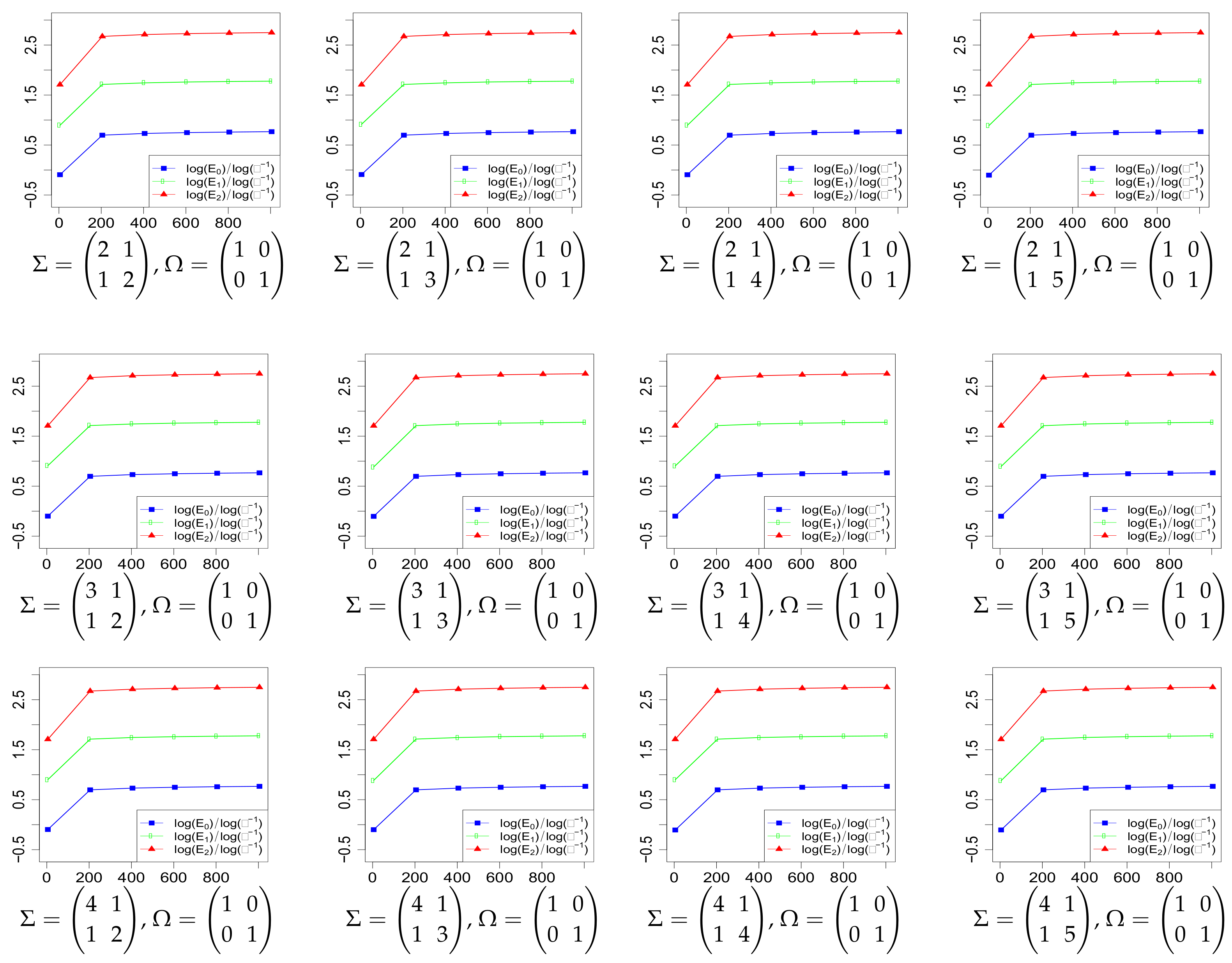
Figure 1. Plots of log E i / log ( ν 1 ) as a function of ν , for various choices of Σ . The plots confirm (5) for our choices of Σ and bring strong evidence for the validity of Theorem 1.
Appliedmath 02 00025 g001
Figure 2. Plots of 1 / E i as a function of ν , for various choices of Σ . Both the horizontal and vertical axes are on a logarithmic scale. The plots clearly illustrate how the addition of correction terms from Theorem 1 to the base approximation (4) improves it.
Appliedmath 02 00025 g002
Publisher’s Note: MDPI stays neutral with regard to jurisdictional claims in published maps and institutional affiliations.