Abstract
In this paper, we extend the block hybrid method with equally spaced intra-step points to solve linear and nonlinear third-order initial value problems. The proposed block hybrid method uses a simple iteration scheme to linearize the equations. Numerical experimentation demonstrates that equally spaced grid points for the block hybrid method enhance its speed of convergence and accuracy compared to other conventional block hybrid methods in the literature. This improvement is attributed to the linearization process, which avoids the use of derivatives. Further, the block hybrid method is consistent, stable, and gives rapid convergence to the solutions. We show that the simple iteration method, when combined with the block hybrid method, exhibits impressive convergence characteristics while preserving computational efficiency. In this study, we also implement the proposed method to solve the nonlinear Jerk equation, producing comparable results with other methods used in the literature.
Keywords:
block hybrid method; equally spaced grid points; differential equations; nonlinear jerk equation; simple iteration method MSC:
65L05
1. Introduction
Differential equations with an appropriate set of conditions are key tools in modeling a plethora of real-world phenomena including engineering problems. It is crucial to have a clear understanding of the behavior and stability of solutions to these differential equations. Many numerical methods have been introduced to find an approximate solution for those cases. In this study, we propose a block hybrid method for the numerical solution of third-order initial value problems (IVPs) of the form
where the prime denotes the derivative with respect to the independent variable z, and f is a continuous linear or nonlinear function in the interval .
Block hybrid algorithms are a class of numerical methods that blend linear multi-step approaches with interpolation using power series. These techniques were first introduced by Gragg and Stetter [1] and Shampine and Watts [2] and involve the inclusion of an additional point within each step of the formula. This allows for more precise approximations of solutions to differential equations, as well as gives better convergence rates. Since the pioneering work of Gear [3], block methods have been extensively studied and used in the literature to solve initial value problems and boundary value problems. Motsa [4] proposed an overlapping grid hybrid block method with equally spaced and optimal grid points for linear and nonlinear first-order IVPs. He found that the overlapping grid approach gave better performance than the standard non-overlapping grid in terms of reducing the local truncation error. Shateyi [5] applied a block hybrid method with equally spaced grid points to solve linear and nonlinear first-order IVPs. He reported that equally spaced grid points provided high rates of convergence outperforming the fourth-order Runge–Kutta method [6]. Orakwelu [7] developed an implicit block hybrid method for solving first-, second-, and third-order IVPs. He investigated the convergence rates, accuracy, and robustness of implicit block hybrid algorithms. He further investigated the performance of these algorithms when various countable off-points were imposed between grid points in the derivation process. El-Hawary and Mahmoud [8] presented the spline functions with four collocation points to solve second-order IVPs. They showed that the spline collocation scheme is convergent with order seven under certain conditions on the collocation point parameters. They found that the stability properties of the method are analyzed rigorously, and regions of absolute stability are determined based on the parameter values.
Various iterative techniques have been discussed for solving initial value and boundary value problems in ordinary and partial differential equations [9,10]. These iterative methods yield the solution or an approximation of it through a sequence of successive iterations. In the case of initial value problems, these iterative approaches can be formulated either in an integral or differential manner [11]. These approaches linearize the nonlinear equations governing the problem around the previous iteration, leading to linear differential equations at each step [12]. However, the coefficients of these equations may vary with the independent variable, necessitating numerical methods for obtaining the approximation solution.
In this study, we are motivated by the work in [4] and propose a block hybrid method for third-order IVPs with equally spaced grid points. Several strategies have been developed in the literature to solve third-order IVPs. For example, Osa et al. [13] used a multi-step block implicit hybrid method. They reported that the block method performed better than predictor–corrector methods [14] in terms of being more time-efficient, cost-effective, and accurate. Rufai and Ramos [15] modified the block method using variable step sizes instead of equally spaced points. They reported that the technique was efficient in terms of computational time and minimized truncation errors. Orakwelu et al. [16] proposed a single-step hybrid block method for solving third-order ODEs without first converting to an analogous first-order system. They reported that the scheme can be implemented without the use of starting values or predictors, avoiding the necessity for complex subroutines method. Several other authors have utilized the equal step size procedure for solving the third-order IVPs [17,18,19].
Block hybrid methods, used to solve differential equations, are primarily applicable to linear equations. However, when dealing with nonlinear equations, the method necessitates a preliminary step of linearization before its implementation. This prerequisite ensures the effectiveness and accuracy of methods when applied to nonlinear equations. In this study, we developed an intra-step equally spaced grid point block hybrid method that is used in conjunction with the simple iteration method (SIM) to solve third-order IVPs. They demonstrated that the SIM linearization technique generates accurate solutions for nonlinear differential equations [20]. The SIM approach is based on transforming a nonlinear ordinary differential equation into an iterative scheme made up of linear equations, which are then solved using a block hybrid method numerical approach. Linearization methods based on truncated Taylor series approximations are employed to simplify the nonlinear terms of nonlinear differential equations. Relaxation methods based on the assumption that nonlinear terms are known from previous iterations can also be used to convert a nonlinear problem to a linear discretizable problem. Newton-based linearization techniques such as the quasi-linearization method [21], local linearization method [22], Keller-box method [23], and relaxation method [24], have extensively been used to linearize differential equations. All these methods are based on one-term Taylor series expansion and are thereby susceptible to series truncation errors even before errors associated with the numerical method used to solve the linearised problem. In this paper, we propose a method that seeks to circumvent the problem of errors associated with linearization. The proposed method uses ideas akin to those of fixed point iteration to develop iterative schemes, called Simple Iteration Methods (SIMs), for solving nonlinear differential equations. Moreover, SIMs are easy to implement. We show the effectiveness of the proposed method (referred to as the SIM-BHM) through numerical experiments, demonstrating that it gives fast convergence and accurate solutions.
2. Development of the SIM-BHM Iterative Method
This section describes the development of the SIM-BHM with equally spaced points for the numerical solution to third-order IVPs (1) and (2). Before starting the development of the hybrid block method, we need to linearize the function f using the SIM scheme as below:
2.1. The SIM Linearization Scheme
In this section, we present the development of the SIM. If the nonlinear equation is rearranged in the form , then an iterative method can be written as
where , and s is the number of iterative steps. This method is called fixed point iteration, the successive substitution method, or the simple iteration method. The simple iteration method is touted as a differential equation equivalent to the fixed point iteration method for solving nonlinear equations. Thus, we begin by reviewing some basic concepts of the fixed point iteration method. The following theorem gives the conditions of the fixed point iteration method.
Theorem 1. (Fixed Point Theorem).
- If g is continuous on a closed interval , for all , then g has at least one fixed point in .
- If, in addition, exists on and a positive constant K exists withthen there is exactly one fixed point in .
Assume that c in is a fixed point for g. Then, if there is an initial guess in , the sequence
converges to the unique fixed point c. For proof of Theorem 1, see [25].
Simple Iteration Method for the ODE
The approach proposed below is a systematic approach based on a rule used to simplify products of unknown functions and their derivatives. We assume that
is a nonlinear function in u, , and . To develop the iteration scheme, Equation (4) is expressed as a sum of its linear as nonlinear components as
The SIM linearization scheme is developed so that the linear component can be written as the sum of linear terms (unknown functions) at iteration
The nonlinear terms are a combination of known (at iteration s) and unknown =functions. In the nonlinear term, the function with a higher derivative is taken as unknown. Provided that the nonlinear component can be written as the sum of nonlinear terms
Substituting Equations (6) and (7) into Equation (5), we obtain
where , and are known functions from a previous iteration given by
Equation (8) is the linearized form of f.
The objective of this paper is to develop an alternative and novel block hybrid method approach that is based on an equally spaced grid (see Figure 1).
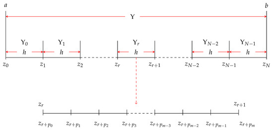
Figure 1.
Illustration of the equally spaced grid points.
We define the block by and the fixed step length or size is denoted by h, where
where N is the number of blocks in . For each block , we define intra-step points as
In using the BHM, we approximate the solution to Equation (1) using a polynomial of the form
In addition, we approximate the first and second derivatives as
respectively, where are unknown coefficients. We apply collocation at the unknown nodes and in Equations (10) and (11). We assume that the approximated solutions (12)–(14) satisfy Equations (1) and (2). The coefficients are obtained from a system of equations with unknowns generated from
where , , , , and . The above system of Equations (15)–(18) can be written in matrix notation as
We solve the above system of Equation (19) to obtain . We use Mathematica code to obtain . The code is as follows
Substituting into Equations (12)–(14) and evaluating the result at collocation points (10) and (11) yield
where , , and are known constants. By substituting Equation (8) into the BHM scheme system of Equations (20)–(22), we obtain a system of equations in matrix form
where
In Equations (23)–(25), is an identity matrix of size (), and all other matrices of size () are defined as follows
whereas vectors of size () are defined as follows
We may rewrite System (25) in compact form as follows
3. Analysis of the Developed SIM-BHM
This section provides the fundamental properties of the proposed SIM-BHM.
3.1. Order and Error Constant
Minimizing the truncation error is a fundamental goal in numerical analysis utilized as a measure to improve the accuracy of the method.
Proposition 1.
In the integration block , for the block hybrid method defined as
the local truncation error is given by
Proof.
Given that u is a sufficiently differentiable function, the local truncation error can be analyzed using the linear operator defined as
where are constant. The method is said to be order q if
where . The vector is the error constant of the method. Using Equation (29), the truncation error of the BHM for third-order can be written in terms of the linear operator as
Expanding the terms and using Taylor series about and then substituting them into Equation (33), we obtain
Following [4,26], we note that
Substituting Equation (37) into Equation (36), we obtain
Using Equation (38), the error constant vector is
where
□
Table 1 shows the truncation error and order for . In the table, we note that increasing the number of intra-step points improves the order of the method.

Table 1.
Truncation errors for the SIM-BHM.
3.2. Zero Stability
The zero stability of the SIM-BHM pertains to the performance of Equation (20) as the step size h approaches zero [27].
Definition 1.
Zero stability is confirmed if the roots of the characteristic polynomial are such that and all roots with have a multiplicity that does not exceed 2.
The characteristic polynomial is given by
In this case, the block hybrid method derived from m equally spaced intra-step points is zero-stable and consistent for any selection of intra-step points.
3.3. Absolute Stability
Definition 2.
A region is said to have absolute stability or be A-stable if it contains the entire left half-plane.
A region of absolute stability for the method can be defined as
Applying the test equation [28]
to the new method gives
where the is given by
The stability function can be determined by finding the dominant eigenvalues of the matrix . The region of absolute stability for this method is shown in Figure 2. The stability function is to be bounded if . The bounded region is illustrated in Figure 3. The BHM is absolute-stable as the stability region contains the entire left half complex plane for .
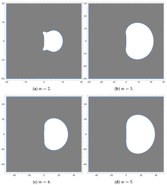
Figure 2.
Region of absolute stability for .
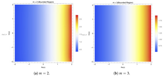
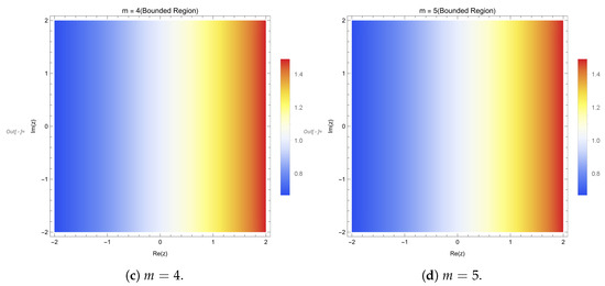
Figure 3.
Region of absolute stability for .
4. Implementation and Computational Procedure of the Proposed SIM-BHM
In this section, we present solutions to third-order IVPs (1)–(2) using the novel SIM-BHM iterative method. In order to evaluate the convergence of the method, we have evaluated the absolute error (AE) and absolute error estimate (AEE) between two consecutive iterations. Suppose and are the approximate solutions. The absolute error is defined as
We compute the absolute error estimate between two consecutive iterations using the following terms
where s represents the solution at the corresponding iteration. We enforce the following conditional stopping procedure in the SIM-BHM iterative method:
- If , the current iteration solutions are deemed satisfactory, and the SIM-BHM proceeds to the next block.
- If , the iteration count is incremented, and the SIM-BHM continues within the same block.
Here, represents the user-defined tolerance. Within each block, the method iterates until the error falls below . Once the converges to within an acceptable criteria, the procedure advances to the next block or concludes the computation. By applying this conditional structure, we ensure that the accuracy of our solutions is systematically improved within each block, thereby enhancing control and precision in our numerical computations.
Algorithm
To illustrate how to implement this SIM-BHM, we demonstrate an algorithm with the steps provided below:
- 1.
- Define function
- Input: Initial value problem function , interval , number of blocks N, tolerance , number of intra-step points m.
- Output: Approximate solution for .
- 2.
- Linearization scheme
- Linearize f by using Equation (8).
- 3.
- Discretization
- Divide interval into N blocks and determine the step size h.
- 4.
- Collocation points
- 5.
- Approximate solutions
- 6.
- Collocation equations
- 7.
- Initialize iteration
- Initialize iteration .
- 8.
- Solve equations
- 9.
- Iterate
- Repeat Steps 7–10 until convergence or maximum iterations reached:
- (a)
- Use Equation (28) to compute approximation solutions , , and at collocation points.
- (b)
- Compute absolute error estimate (AEE) between consecutive iterations using Equation (45).
- (c)
- If , , and , accept solutions and move to next block (Step 10).
- (d)
- If , , and , reject solutions and increase iteration s by 1.
- 10.
- Output
- Output the approximate solutions , , and at the block r.
5. Numerical Experimentation
In the next section, we test the method by implementing the SIM-BHM with some specific third-order IVPs from the literature.
Example 1.
Consider the linear third-order IVP [13,17,18,19]
This IVP has the exact solution: .
Here, we selected , and to implement the SIM-BHM6 scheme, we defined
In Table 2, we compare the maximum absolute errors of the SIM-BHM6 method with different variants of the hybrid block method [13,17,18,19]. Adesanya et al. [17] used the block method with six collocation points, Areo et al. [18] used the one-twelfth multi-step block method, Skwame et al. [19] used the equally spaced block method with five collocation points, and Osa et al. [13] used the multi-step block method with fifth–fourth collocation points. It is evident that the SIM-BHM6 consistently outperforms the existing block methods in terms of reducing maximum absolute errors. Figure 4 showcases the number of iterations required in each block. The result provides strong evidence of the impressive convergence properties of SIM-BHM6, achieving good accuracy in just two iterations when across all blocks, as shown in Figure 4a,b. It is particularly noteworthy that the method attains a high level of accuracy while maintaining computational efficiency.
Table 2.
Maximum absolute error comparison using SIM-BHM6.
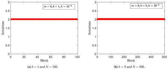
Figure 4.
Iterations per block using the SIM-BHM6.
Example 2.
Consider the linear third-order IVP [15,29,30]
The exact solution: .
In this example, we used SIM-BHM6 with
Table 3 gives a comparison of the maximum absolute errors using the SIM-BHM6 method with different variants of the block method [15,29,30]. As shown in Table 3, Rufai and Ramos [15] used a variable step-size fourth-derivative block method, Awoyemi1 et al. [29] used a linear multi-step block method with five collocation points, and Allogmany and Ismail [30] used a fourth and fifth derivative block method with three implicit collocation points. We note that SIM-BHM6 outperformed the other block methods in terms of reducing maximum absolute errors. Figure 5 shows that the method achieves good accuracy in two iterations for across all blocks.
Table 3.
Maximum absolute error comparison for SIM-BHM6 when .
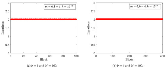
Figure 5.
Iterations per block using SIM-BHM6.
Example 3.
Consider the nonlinear third-order IVP [31]
The exact solution of Example 3 is .
In this example, we selected , , and . We define
In Table 4, we present a comparative analysis of the maximum absolute errors achieved using the SIM-BHM4, SIM-BHM5, and SIM-BHM6 methods with the work in [31]. Adeyeye and Omar [31] employed a block method with equally spaced collocation points. Notably, our findings show enhancement in accuracy when adopting SIM-BHM, particularly as we increase the number of intra-step points and reduce the step sizes. Figure 6a–c provide a visual representation of the number of iterations required across various blocks. In the case of shorter intervals, as in Figure 6a with 10 blocks, we observe that the maximum number of iterations required is five. As shown in Figure 6b, when 100 blocks are utilized, the maximum number of iterations reduces to four. These observations underscore the role of smaller step sizes in reducing the maximum iteration count within the blocks. For larger intervals, as illustrated in Figure 6a with 300 blocks, the maximum number of iterations remains at five. This suggests that, even in scenarios with a larger solution domain, the SIM-BHM maintains its efficient convergence characteristics. Figure 6d provides further evidence of SIM-BHM’s effectiveness, indicating that the method returns a maximum absolute error less than . This level of precision underscores the robustness and accuracy of the SIM-BHM approach. SIM-BHM6 generally outperforms both SIM-BHM4 and SIM-BHM5.
Table 4.
Maximum absolute error comparison for SIM-BHM4, SIM-BHM5, and SIM-BHM6.
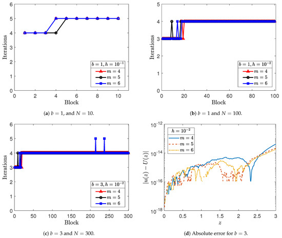
Figure 6.
Iterations per block and absolute error for SIM-BHM when , , and .
Example 4.
Consider a nonlinear system of third-order IVPs [15]
with the exact solutions given as , , and .
In the case of a system of equations, the SIM-BHM6 parameters are given by
Table 5 shows a comparison of the maximum absolute errors achieved using SIM-BHM6 with the work of Rufai and Ramos [15]. Table 5 illustrates the superior accuracy and computational efficiency of SIM-BHM6 compared to the methodology proposed in [15]. SIM-BHM6 consistently yields more precise approximate solutions across a range of scenarios while maintaining efficient computational performance. Figure 7 provides a representation of the maximum iterations within the computational blocks. Notably, the reduction in user-defined tolerance led to an increase in the number of iterations between the blocks. We observed a maximum of six iterations. Figure 8 gives a comparison of the exact vs. numerical of the displacements in Figure 8a and phase portrait in Figure 8b.
Table 5.
Maximum absolute error comparison using the SIM-BHM6.
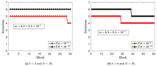
Figure 7.
Iterations per block using SIM-BHM6 when and .
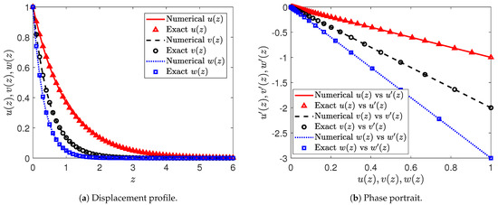
Figure 8.
Numerical solution vs. exact solution using SIM-BHM6 when , , and .
Example 5.
Consider a nonlinear IVP [13] given as
with the exact solution:
In this example, we use SIM-BHM4 with
Table 6 provides a comprehensive comparison between the maximum absolute errors achieved using the SIM-BHM4 method and the results obtained by Osa and Olaoluwa [13]. Figure 9 illustrates the number of iterations within the computational blocks for different values of b for a tolerance . The maximum number of iterations required was for short and large intervals. The corresponding absolute error profiles for , and are plotted in Figure 10a. Figure 10b shows the exact vs. numerical solution for , , and .
Table 6.
Maximum absolute errors comparison for SIM-BHM4 when .
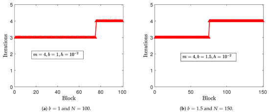
Figure 9.
Iterations per block using the SIM-BHM4 when .
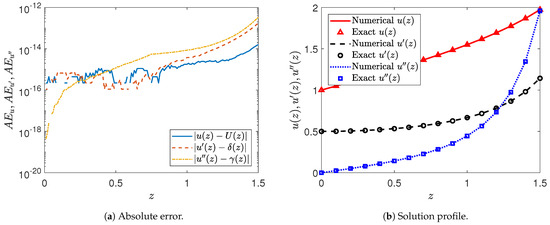
Figure 10.
Absolute error and numerical solution vs. exact solution using the SIM-BHM4 when , , and .
6. On the Application of the SIM-BHM to Solve Nonlinear Jerk Equations
The concept of jerk is particularly relevant in the study of motion and control systems, especially in engineering and physics [32,33]. In physics, the jerk equation models particle motion under varying forces, providing valuable insights into dynamic systems [34]. The equation is used to model systems where the rate of change in acceleration is important, such as in vibration analysis, control systems, and motion planning. Additionally, jerk analysis finds application in signal processing and control theory, facilitating the filtering of noisy signals and the detection of anomalies, contributing to technological advancements. Higher derivatives of motion, such as snap, are also important in motion control and can be experienced in everyday life, such as on trampolines and roller coasters [35].
We consider a class of nonlinear jerk equation IVP containing a third derivative of position with respect to time that describes the rate of change in acceleration, and it is given by
where the parameters , , , , , and are constant. Since there is no analytic solution to Equation (46), we compared the results of the solution profiles to approximated solutions that have been previously reported in the literature [36,37,38,39].
- Gottlieb [38] employed the harmonic balance method (HBM) approach approximation solution to solve the nonlinear Equation (48). He found that HBM yields a good approximated solution of the period and displacement amplitude of oscillations for a range of values of initial velocity, given aswhere is the angular frequency. To solve Equation (48) numerically, we use SIM-BHM7 withCase 1 is solved using SIM-BHM7 with and in the domain of integration . The displacement and phase trajectory are given in Figure 11a and Figure 11b, respectively. A comparison of the approximated analytical vs. numerical solution is depicted by plotting the two results on the same graph. The corresponding iterations per block and the absolute error profiles for the displacement are plotted in Figure 12a and Figure 12b, respectively, for different values of the initial velocity .
- Case 2: , and . For the Case 2 values of the parameters, the nonlinear jerk Equation (46) is given asMirzabeigy and Yildirim [39] employed the modified differential transform method (MDTM) to obtain approximate periodic solutions to Equation (50), given asIn Case 2, we employ SIM-BHM3 withTo determine the accuracy of SIM-BHM3, the numerical results are compared with Kashkari and Alqarni [40]. In their work, they implemented a two-step hybrid block method (TSHBM) with a polynomial of degree 6. Table 7 gives a comparison of the SIM-BHM for and . It can be observed that SIM-BHM3 gives similar results to MDTM and TSHBM within a fast CPU time.
Table 7. Comparison of implementation the SIM-BHM3 when , , and .
Figure 13a depicts the number of iterations required per block for different values of the initial velocity . It can be observed that SIM-BHM3 converges within five iterations. Figure 13b illustrates the phase portrait for different values of the initial velocity.
- Case 3: , , and .Here, we setThe displacement, velocity, acceleration, and phase portrait trajectories are given in Figure 14. A comparison of the exact (MDTM) vs. numerical (SIM-BHM3) solutions is depicted by plotting the two results on the same graph. The corresponding phase portrait and iterations per block are plotted in Figure 15a and Figure 15b, respectively, for different values of .
- With linearization, we obtainEquation (54) is solved using SIM-BHM7 with in the domain of integration for different values of the initial velocity . The displacement and iterations per block utilized to solve Equation (54) are plotted in Figure 16 for different values of the initial velocity.Figure 17 depicts phase portraits for Case 4 when varying .
- With linearization, we obtain
We considered five cases of nonlinear jerk Equation (46) with different parameter combinations for Equations (48)–(56). This allowed us to test the SIM-BHM approach on various forms of the jerk equation. For Cases 1–3, known analytical solutions from previous works were available to validate our numerical results. The SIM-BHM-produced displacement profiles, velocities, accelerations, and phase portraits are in agreement with these established solutions. In Cases 4 and 5, there were no analytical solutions. The SIM-BHM generated physically realistic oscillatory behaviors as the initial velocity parameter was varied. This indicates that the method can reliably solve these types of jerk equations numerically. Across all test cases, the SIM-BHM converged rapidly, typically requiring only 2–8 iterations per block. Even for large solution domains and higher values producing larger oscillations, the method maintained its fast convergence. The displacement profiles, phase portraits, and plots of the iterations clearly illustrate the accuracy and consistency of the SIM-BHM approach. Comparisons with previous works validated the high precision of the numerical solutions obtained. In conclusion, the SIM-BHM proves to be an effective technique for solving an important class of nonlinear jerk equations. It generates solutions in close agreement with the known results. The method exhibits robust computational performance and accuracy across a wide range of problem scenarios.
The numerical experiments consistently showed the SIM-BHM achieving higher accuracy when a smaller step size h was used. For example, reducing h from to led to errors 1–2 orders of magnitude smaller across test problems. This implies that the method exhibits the expected property of increased accuracy for smaller discretization. Larger solution domains were also handled effectively. Cases 1–3 of the jerk equations covered intervals up to with good precision. Cases 4 and 5 were solved over the wider range of while maintaining accuracy. The SIM-BHM modeled problems requiring integration over large physical spaces. Additional support comes from Example 5, where accuracy improved for the longer interval of compared to . These examples provide strong evidence that SIM-BHM’s accuracy increases predictably with smaller h and can be systematically extended to large b values through domain discretization.

Figure 11.
Displacement and phase trajectory for using SIM-BHM7 when , , , and .
Figure 11.
Displacement and phase trajectory for using SIM-BHM7 when , , , and .


Figure 12.
Iterations per block and absolute error for using the SIM-BHM7 when , , , , and .
Figure 12.
Iterations per block and absolute error for using the SIM-BHM7 when , , , , and .


Figure 13.
Displacement and phase trajectory for using the SIM-BHM3 when , , , and .
Figure 13.
Displacement and phase trajectory for using the SIM-BHM3 when , , , and .


Figure 14.
Displacement, velocity, acceleration, and phase portrait for using the SIM-BHM3 when , , , , and .
Figure 14.
Displacement, velocity, acceleration, and phase portrait for using the SIM-BHM3 when , , , , and .


Figure 15.
Displacement and phase trajectory for using SIM-BHM3 when .
Figure 15.
Displacement and phase trajectory for using SIM-BHM3 when .


Figure 16.
Displacement and iterations per block for using SIM-BHM7 when , , and .
Figure 16.
Displacement and iterations per block for using SIM-BHM7 when , , and .


Figure 17.
Phase trajectory for using the SIM-BHM7 when , , and .
Figure 17.
Phase trajectory for using the SIM-BHM7 when , , and .


Figure 18.
Displacement and iterations per block for using SIM-BHM7 when , , and .
Figure 18.
Displacement and iterations per block for using SIM-BHM7 when , , and .


Figure 19.
Phase portraits for using SIM-BHM7 when , , and .
Figure 19.
Phase portraits for using SIM-BHM7 when , , and .

7. Conclusions
We introduced a novel SIM-BHM iterative method for solving third-order IVPs with a fixed step size. The primary objective of the SIM-BHM is to obtain accurate solutions to the IVPs. To evaluate the convergence of the method, we evaluated the absolute error and the absolute error estimate between consecutive iterations. We applied the SIM-BHM to a variety of IVPs, both linear and nonlinear. We compared its performance with existing block methods. The results consistently demonstrated the superior performance of the SIM-BHM in terms of returning the lowest maximum absolute errors, highlighting its accuracy and efficiency. The SIM-BHM offers a versatile approach by employing a selective intra-step method and ensuring convergence. The method gives highly accurate solutions with good computational performance. The main findings with regard to this numerical method are as follows:
- Smaller intra-step sizes generally lead to smaller truncation errors.
- Increasing the number of collection points improves the accuracy of SIM-BHM.
- For large intervals, the SIM-BHM gave more accurate approximations than some existing BHMs, for example, those in [13,15,17,18,19,29,30,31].
- The SIM-BHM gives robust computational performance using only a few iterations.
The SIM-BHM method was applied to solve nonlinear jerk equations. Jerk equations are an important class of third-order problems with applications in fields like engineering and physics. Five cases of jerk equations with varying parameter combinations were tested. Comparisons to known approximate solutions from previous works showed excellent agreement for Cases 1–3. The method generated physically realistic oscillatory behaviors for Cases 4 and 5. Across all jerk equation problems, the SIM-BHM maintained its fast convergence, typically requiring only a few iterations per block even for large solution domains and higher oscillation amplitudes. The accuracy of the numerical solutions was validated through comparisons. This demonstrates the SIM-BHM provides an effective technique for reliably solving nonlinear jerk equations.
In future work, the following would allow for improving the performance of the SIM-BHM:
- Implementing adaptivity with variable step size would allow the method to better capture solutions with varying behaviors over the domain. This could enhance accuracy.
- Investigating the use of Legendre–Gauss–Lobatto and Gauss–Lobatto collocation points, which have been shown to improve accuracy.
- Applying optimally spaced intra-step points within each block, as studies have observed non-uniform point distributions lead to higher precision than uniform spacing [7].
- Applying the overlapping domain approach, where blocks intersect, as this has been demonstrated to reduce errors versus standard non-overlapping grids [4,41].
- Extending the SIM-BHM framework to other problem types, such as higher-order initial value problems, boundary value problems, singular differential equations, and fractional differential equations, to evaluate performance on broader classes of equations.
Author Contributions
Conceptualization, S.A.A.A.A.A.; Investigation, S.A.A.A.A.A. and U.O.R.; Writing—original draft, S.A.A.A.A.A.; Writing—review & editing, P.S., S.P.G., H.S.M. and O.A.I.N.; Supervision, P.S., S.P.G. and O.A.I.N. All authors have read and agreed to the published version of the manuscript.
Funding
This research was funded by the University of KwaZulu-Natal.
Data Availability Statement
Data are contained within the article.
Conflicts of Interest
The authors declare no conflicts of interest.
Abbreviations
The following abbreviations are used in this manuscript:
| AE | Absolute error |
| AEE | Absolute error estimate |
| BHM | Block hybrid method |
| HBM | Harmonic balance method |
| MDTM | Modified differential transform method |
| ODE | Ordinary differential equation method |
| TSHBM | Two-step hybrid block method |
| Max AE | Largest absolute error |
| SIM | Simple iteration method |
References
- Gragg, W.B.; Stetter, H.J. Generalized multistep predictor-corrector methods. J. Assoc. Comput. Mach. 1964, 11, 188–209. [Google Scholar] [CrossRef]
- Shampine, L.F.; Watts, H. Block implicit one-step methods. Math. Comput. 1969, 23, 731–740. [Google Scholar] [CrossRef]
- Gear, C.W. Hybrid methods for initial value problems in ordinary differential equations. J. Soc. Ind. Appl. Math. Ser. B Numer. Anal. 1965, 2, 69–86. [Google Scholar] [CrossRef]
- Motsa, S. Overlapping Grid-Based Optimized Single-Step Hybrid Block Method for Solving First-Order Initial Value Problems. Algorithms 2022, 15, 427. [Google Scholar] [CrossRef]
- Shateyi, S. On the Application of the Block Hybrid Methods to Solve Linear and Non-Linear First Order Differential Equations. Axioms 2023, 12, 189. [Google Scholar] [CrossRef]
- Burden, R.; Faires, J. Numerical Analysis, 9th ed.; Cengage Learning: Boston, MA, USA, 2011. [Google Scholar]
- Orakwelu, M.G. Generalised Implicit Block Hybrid Algorithms for Initial Value Problems. Ph.D. Thesis, University of KwaZulu-Natal, Peitermaritzburg, South Africa, 2019. [Google Scholar]
- El-Hawary, H.; Mahmoud, S. On some 4-point spline collocation methods for solving second-order initial value problems. Appl. Numer. Math. 2001, 38, 223–236. [Google Scholar] [CrossRef]
- Bellman, R.E.; Kalaba, R.E. Quasilinearization and Nonlinear Boundary-Value Problems; Elsevier: New York, NY, USA, 1965. [Google Scholar]
- Mandelzweig, V.; Tabakin, F. Quasilinearization approach to nonlinear problems in physics with application to nonlinear ODEs. Comput. Phys. Commun. 2001, 141, 268–281. [Google Scholar] [CrossRef]
- Kelley, C.T. Iterative Methods for Linear and Nonlinear Equations; SIAM: Philadelphia, PA, USA, 1995. [Google Scholar]
- Ramos, J.I. On the variational iteration method and other iterative techniques for nonlinear differential equations. Appl. Math. Comput. 2008, 199, 39–69. [Google Scholar] [CrossRef]
- Osa, A.L.; Olaoluwa, O.E. A fifth-fourth continuous block implicit hybrid method for the solution of third order initial value problems in ordinary differential equations. Appl. Comput. Math 2019, 8, 50–57. [Google Scholar]
- Butcher, J.C. Numerical Methods for Ordinary Differential Equations; John Wiley & Sons: Hoboken, NJ, USA, 2016. [Google Scholar]
- Rufai, M.A.; Ramos, H. A variable step-size fourth-derivative hybrid block strategy for integrating third-order IVPs, with applications. Int. J. Comput. Math. 2022, 99, 292–308. [Google Scholar] [CrossRef]
- Orakwelu, M.G.; Otegbeye, O.; Mambili-Mamboundou, H. A class of single-step hybrid block methods with equally spaced points for general third-order ordinary differential equations. J. Niger. Soc. Phys. Sci. 2023, 5, 1484. [Google Scholar] [CrossRef]
- Adesanya, A.O.; Udoh, D.M.; Ajileye, A. A new hybrid block method for the solution of general third order initial value problems of ordinary differential equations. Int. J. Pure Appl. Math. 2013, 86, 365–375. [Google Scholar] [CrossRef]
- Areo, E.; Omojola, M. One-Twelveth Step Continuous Block Method. Int. J. Pure Appl. Math. 2017, 114, 165–178. [Google Scholar] [CrossRef][Green Version]
- Skwame, J.; Dalatu, P.; Sabo, J.; Mathew, M. Numerical application of third derivative hybrid block methods on third Order Initial Value Problem of ordinary differential equations. Int. J. Stat. Appl. Math. 2019, 4, 90–100. [Google Scholar]
- Otegbeye, O.; Ansari, M.S. A finite difference based simple iteration method for solving boundary layer flow problems. AIP Conf. Proc. 2022, 2435, 020055. [Google Scholar]
- Parsaeitabar, Z.; Nazemi, A. A Third-degree B-spline Collocation Scheme for Solving a Class of the Nonlinear Lane—Emden Type Equations. Iran. J. Math. Sci. Inform. 2017, 12, 15–34. [Google Scholar]
- Motsa, S.S. A new spectral local linearization method for nonlinear boundary layer flow problems. J. Appl. Math. 2013, 2013, 423628. [Google Scholar] [CrossRef]
- Keller, H.B.; Cebeci, T. Accurate numerical methods for boundary-layer flows. II: Two dimensional turbulent flows. AIAA J. 1972, 10, 1193–1199. [Google Scholar] [CrossRef]
- Zubik-Kowal, B.; Vandewalle, S. Waveform relaxation for functional-differential equations. SIAM J. Sci. Comput. 1999, 21, 207–226. [Google Scholar] [CrossRef]
- Burden, A.M.; Burden, R.L.; Faires, J.D. Numerical Analysis, 10th ed.; Cengage Learning: Boston, MA, USA, 2016. [Google Scholar] [CrossRef]
- Butcher, J.C. Implicit Runge–Kutta processes. Math. Comput. 1964, 18, 50–64. [Google Scholar] [CrossRef]
- Lambert, J.D. Computational Methods in Ordinary Differential Equations; Wiley: London, UK, 1973. [Google Scholar]
- Dahlquist, G. Convergence and stability in the numerical integration of ordinary differential equations. Math. Scand. 1956, 4, 33–53. [Google Scholar] [CrossRef]
- Awoyemi, D.; Kayode, S.; Adoghe, L. A five-step P-stable method for the numerical integration of third order ordinary differential equations. Am. J. Comput. Math. 2014, 4, 119–126. [Google Scholar] [CrossRef][Green Version]
- Allogmany, R.; Ismail, F. Implicit three-point block numerical algorithm for solving third order initial value problem directly with applications. Mathematics 2020, 8, 1771. [Google Scholar] [CrossRef]
- Adeyeye, O.; Omar, Z. Solving third order ordinary differential equations using one-step block method with four equidistant generalized hybrid points. Int. J. Appl. Math. 2019, 49, 1–9. [Google Scholar]
- Kyriakopoulos, K.J.; Saridis, G.N. Minimum jerk path generation. In Proceedings of the 1988 IEEE International Conference on Robotics and Automation, Philadelphia, PA, USA, 24–29 April 1988; pp. 364–369. [Google Scholar]
- Hayati, H.; Eager, D.; Pendrill, A.M.; Alberg, H. Jerk within the context of science and engineering—A systematic review. Vibration 2020, 3, 371–409. [Google Scholar] [CrossRef]
- Eichhorn, R.; Linz, S.J.; Hänggi, P. Transformations of nonlinear dynamical systems to jerky motion and its application to minimal chaotic flows. Phys. Rev. E 1998, 58, 7151. [Google Scholar] [CrossRef]
- Eager, D.; Pendrill, A.M.; Reistad, N. Beyond velocity and acceleration: Jerk, snap and higher derivatives. Eur. J. Phys. 2016, 37, 065008. [Google Scholar] [CrossRef]
- Gottlieb, H. Simple nonlinear jerk functions with periodic solutions. Am. J. Phys. 1998, 66, 903–906. [Google Scholar] [CrossRef]
- Liu, C.S.; Chang, J.R. The periods and periodic solutions of nonlinear jerk equations solved by an iterative algorithm based on a shape function method. Appl. Math. Lett. 2020, 102, 106151. [Google Scholar] [CrossRef]
- Gottlieb, H. Harmonic balance approach to periodic solutions of non-linear jerk equations. J. Sound Vib. 2004, 271, 671–683. [Google Scholar] [CrossRef]
- Mirzabeigy, A.; Yildirim, A. Approximate periodic solution for nonlinear jerk equation as a third-order nonlinear equation via modified differential transform method. Eng. Comput. 2014, 31, 622–633. [Google Scholar] [CrossRef]
- Kashkari, B.S.; Alqarni, S. Two-step hybrid block method for solving nonlinear jerk equations. J. Appl. Math. Phys. 2019, 7, 1893. [Google Scholar] [CrossRef][Green Version]
- Mkhatshwa, M.P. Overlapping Grid Spectral Collocation Methods for Nonlinear Differential Equations Modelling Fluid Flow Problems. Ph.D. Thesis, University of KwaZulu-Natal, Peitermaritzburg, South Africa, 2020. [Google Scholar]


Disclaimer/Publisher’s Note: The statements, opinions and data contained in all publications are solely those of the individual author(s) and contributor(s) and not of MDPI and/or the editor(s). MDPI and/or the editor(s) disclaim responsibility for any injury to people or property resulting from any ideas, methods, instructions or products referred to in the content. |
© 2024 by the authors. Licensee MDPI, Basel, Switzerland. This article is an open access article distributed under the terms and conditions of the Creative Commons Attribution (CC BY) license (https://creativecommons.org/licenses/by/4.0/).