Measuring the Risk of Vulnerabilities Exploitation

Abstract

Modeling the vulnerabilities lifecycle and exploitation frequency are at the core of security of networks evaluation. Pareto, Weibull, and log-normal models have been widely used to model the exploit and patch availability dates, the time to compromise a system, the time between compromises, and the exploitation volumes. Random samples (systematic and simple random sampling) of the time from publication to update of cybervulnerabilities disclosed in 2021 and in 2022 are analyzed to evaluate the goodness-of-fit of the traditional Pareto and log-normal laws. As censoring and thinning almost surely occur, other heavy-tailed distributions in the domain of attraction of extreme value or geo-extreme value laws are investigated as suitable alternatives. Goodness-of-fit tests, the Akaike information criterion (AIC), and the Vuong test, support the statistical choice of log-logistic, a geo-max stable law in the domain of attraction of the Fréchet model of maxima, with hyperexponential and general extreme value fittings as runners-up. Evidence that the data come from a mixture of differently stretched populations affects vulnerabilities scoring systems, specifically the common vulnerabilities scoring system (CVSS).

1. Introduction

A vulnerability is a weakness, for instance a design flaw or an implementation bug, that can be exploited to threaten a computer system, resulting in the stealing of data, installation of malware, or the running of malicious code. Cybervulnerabilities are a major economic concern. Their severity and the risk of consequent exploitation guide the prioritization of those needing urgent patching or remediation. From 2005 onwards, the common vulnerabilities scoring system (CVSS) [1], using base, temporal, and environmental metrics, has been a standard approach for assessing the severity of vulnerabilities, particularly in the banking sector, although its usefulness is compromised, since the use of temporal and environmental metrics is optional. Moreover, the fact that it is static is subject to harsh criticism, since it is clear that risk changes over time. Modeling the vulnerabilities lifecycle and exploitation frequency are at the core of security of networks evaluation. Pareto, Weibull, and log-normal models have been widely used to model exploit and patch availability dates, the time to compromise a system, the time between compromises, and the exploitation volumes. As malware rarely causes significant damage, propagates at high speed, and is difficult to remove, the risk associated for most vulnerabilities is low, while there can be many missing values in the records, compromising the validity of the analysis of data.

As the existing data arguably result from drastic censoring and eventual thinning, thus representing top- or bottom-order statistics, other heavy-tailed distributions in the domain of attraction of extreme value or geo-extreme value laws are investigated as suitable alternatives to the Pareto model, power law models, and log-normal models.

Section 2 sketches some of the main features of vulnerabilities threats, and of the main scoring systems, including the CVSS and the exploit prediction scoring system (EPSS), evaluating their severity and the consequent risk of exploitation. The sophisticated machine learning algorithm, EPSS, for computing the probability of a vulnerability being exploited in the wild, uses more than one thousand variables in its algorithm black box, as well as the number of days since disclosure. The time variables in the lifecycle of vulnerabilities are crucial to understand the exposure risk of a network, and a main feature of this work is a critical appraisal of the goodness-of-fit of heavy-tailed distributions to the time from publication to the update of vulnerabilities.

In Section 3, progress in the statistical analysis of heavy-tailed empirical data from variables arising in the management of vulnerabilities and the associated risk and remediation are analyzed. The detailed discussion provided by Frei et al. [2], Holm [3], and Allodi [4] highlight the modeling of several time variables in the lifecycle of vulnerabilities, while Ruohonen [5] and references therein, serve as a basis for understanding the evolution of the state of the art in this matter.

In Section 4, several heavy-tailed laws for modeling the time variables in the lifecycle of vulnerabilities are discussed. The main idea is that extreme value models may have advantages over traditional power laws. On the other hand, as there exists strong evidence that thinning in the reporting of data certainly does occur, instead of use of the traditional general extreme value (GEV) model, or of the associated generalized Pareto model, use of the geo-max laws introduced by Rachev and Resnick [6], namely the log-logistic heavy-tailed law in the domain of attraction of the Fréchet law of long-tailed maxima, may represent a valuable approach. As the data exhibit some features typical of mixture models, and in light of the claims of Feldmann and Whitt [7] in favor of long-tail mixtures of exponentials, hyperexponential models are also discussed.

In Section 5, information on the process of obtaining the samples of vulnerabilities reported in [8] that are used in the analyzes is provided. Some issues concerning model fitting and parameter estimation, and the criteria for model choice, namely the Akaike information criterion (AIC) [9], the Schwarz–Bayesian information criterion (BIC) [10], and Vuong’s test [11], are briefly sketched.

In Section 6, the goodness-of-fit of the models under evaluation is compared with regards to the time from publication to the update of vulnerabilities sampled from 2021 and 2022. The general result, both for the 2021 systematic sample and for the 2022 simple random sample without replacement, is that power law fitting is inadequate, and that, as predicted from considerations on extreme values and thinning, the log-logistic model provides the best fit. On the other hand, a hyperexponential fit can be strongly recommended, since there is evidence that the data come from at least two differently stretched distributions.

Section 7 draws the conclusions from the statistical analysis, with suggestions provided regarding overcoming the static status of the CVSS, and discusses the evolution of metrology towards the consideration of virtual metrics.

In the Appendices, some further information on the CVSS metrics and evolution towards version 4.0, to be released soon, and on the Pareto laws is provided.

2. Vulnerabilities and Scoring Systems

Vulnerabilities are weaknesses that can be exploited by cybercriminals to access a computer system, with the intention of running malicious code, stealing sensitive data, and/or installing malware (Tunggal [12]), creating risks of possible intrusion and exploitation with potentially serious economic losses (Eling et al. [13]).

The first two vulnerabilities were reported in 1988. Nowadays, the Vulnerability Database [14] contains 236,311 vulnerabilities, with 25,227 vulnerabilities registered in 2022 in the National Vulnerability Database [15] from NIST, the National Institute of Standards and Technology. Information held in the Exploit Database [16] shows that until 7 August 2023, 5710 vulnerabilities exploitation codes had been detected, and that 33,750 had been verified. In Figure 1, a huge increase in the yearly disclosure of vulnerabilities can be observed, mainly occurring since 2017.

The probability of a vulnerability being maliciously exploited and the impact of eventual exploits (meaning the likelihood of an intrusion occurring) are decisive in assessing the risk it represents. It is assumed that on a monthly basis from 5 to 20% of known vulnerabilities are corrected, while only 2 to 7% of vulnerabilities are actually exploited (Usingdata from [8], the percentage of exploited vulnerabilities is only 1.87%, with very high percentages observed between 2009 and 2012 (see Appendix C). However, apparently these data refer to vulnerabilities following assignment of a common vulnerabilities and exposures ID (CVE-ID), and the greatest risk occurs in the pre-disclosure period). Allodi [4] indicates that between 2009 and 2012, approximately 95% of the $75.7\times {10}^6$ attacks on 374 vulnerabilities targeted only 5% of them, which led him to comment that panic reactions are inappropriate, stating, “[…] most vulnerabilities may carry negligible risk. This indicates that the classical approach ’I have a vulnerability’ → `I must fix it’ may be a largely disproportionate reaction to the real threat.”

The percentage of vulnerabilities subject to cyberattacks seems low, but as nowadays more than 20,000 new vulnerabilities appear annually, it is anticipated that around 400 to 1700 of them may be subject to exploitation.

The eventual losses for companies, expenses associated with cybersecurity, and the existence of a flourishing market for instruments facilitating the exploitation of vulnerabilities, has drawn attention to the economic importance of the issue, with the potential for extreme negative outcomes (Eling et al. [13]). Therefore, it is essential to highlight the vulnerabilities that may potentially represent greater risks in order to prioritize those requiring urgent remediation or mitigation (which may not represent conclusive solutions), or, ideally, patching.

CVSS and Other Tools for Assessing the Severity and Risk of Vulnerabilities

Vulnerabilities have a strong bearing on the security level of networks, and CVSS has been widely used to assess the severity rating of security risks since version 1 appeared in 2005.

CVSS version 3.1 (released in June 2019) considers a base metric group (exploitability metrics and impact metrics) of eight nominal variables, a temporal metric group of three nominal variables, and an environmental metric group of 11 nominal variables, producing string vectors (check the CVSS v3.1 calculator at [1]). Each metric category has a corresponding numerical value, and a score is produced using the CVSS v3.1 equations (see details in Appendix A). Although the number of possible string vectors, 191,102,976,000, is very large, due to roundup procedures and limitation of the range to [0,10], only 101 scores are theoretically possible, leading to a qualitative severity rating scale considering the level of risk as follows: None $\leftrightarrow 0$, Low $\leftrightarrow [0.1,3.9]$, Medium $\leftrightarrow [4.0,6.9]$, High $\leftrightarrow [7.0,8.9]$, and Critical $\leftrightarrow [9.0,10.0]$.

The ’High’ and ’Critical’ severity ratings indicate vulnerabilities that can have a significant economic impact. Papers on the economic consequences of vulnerability exploits, such as Anderson [17], Bollinger [18], Dubendorfer et al. [19], and Kannan and Telang [20], had surely some bearing on moving from the 2005 Qualys [21] qualitative evaluation of the laws of vulnerabilities towards the quantitative score assessment of CVSS. With regard to the economic effect of vulnerabilities, the paper by Anderson and Mood [22] appeared before the release of CVSS v2 in 2007, while Frei’s comprehensive doctoral dissertation [23] had already been submitted in 2009.

Although CVSS scores are widely used to assess the severity of vulnerabilities, it must be noted that the optional temporal and environmental metrics are seldom used. Moreover, the temporal metrics do not reflect the fact that risk associated with vulnerabilities changes over time. As the optional temporal metrics of CVSS v3.1 did not effectively impact the CVSS score, v4.0 (to be released later in 2023) substitutes these with threat metrics. Additional attributes for vulnerability response are also introduced in v4.0 (cf. Appendix B). The effect of the temporal metrics equation in CVSS v3.1 is to produce a temporal score $\mathrm{TS}=\mathrm{RUp}\left(\mathrm{BS}\times \mathrm{ECM}\times \mathrm{RL}\times \mathrm{RC}\right)$, with BS denoting the basic score, ECM, the exploit code maturity, RL, the remediation level, RC, the report confidence, and RUp, the ceiling decimal round up, which can reduce the base score by up to 79.5334% (cf. Appendix A). As a consequence, other methodologies to evaluate the vulnerability severity and ensuing exploitation risk have been devised. Mention should also be made of other tools described below.

EPSS:

EPSS registers the probability that a vulnerability will be exploited, with an additional indication of the corresponding percentile. The calculation of these probabilities is performed by an algorithm based on machine learning using 1164 variables covering a wide spectrum of information, including the CVSS base score and the number of days that have elapsed since disclosure (see detailed description in [24], and in Jacobs et al. [25]). The training for version 2 used gradient boosting and Poisson regression. Version 3 was released in March 2023.

The probability indicated by EPSS is a guide to identifying vulnerabilities that should be prioritized in the remediation effort. Note that, since it is a probability, false negatives and false positives must be taken into account.

The strengths of EPSS are its ability to calculate the probability of risk of a set of vulnerabilities, and consequently the probability that a company is at risk of exploitation when using software subject to a set of vulnerabilities. In addition, the fact that the calculation is dynamic, which is a consequence of the algorithm being automatically updated taking into account new information, represents a further advantage. For example, vulnerability CVE-2021-44228 (CVSS score 10), published on 10 December 2021, started with an exploit probability estimated by EPSS at 0.355 on 11 December. On 13 December, it became 0.384, on 14 December, 0.300, on 15 December, it increased to 0.633, on 17 December to 0.944, on 18 December, it dropped to 0.633, but on 12 January 2022, it increased again to 0.944.

However, the EPSS only exists for previously published vulnerabilities—there is no calculator that can be used in the CVE-ID discovery/reservation phase as exists for the CVSS.

An efficiency comparison of CVSS v3.1, EPSS v1, and EPSS v2 considering the November 2021 vulnerabilities showed, respectively, scores greater than 8.6, probabilities greater than 0.066, and probabilities exceeding 0.149, in order to provide coverage of around 50% in the three scenarios, as described in the documentation on the EPSS model. These thresholds led to signaling for corrections of 25.3%, 9.3%, and 4.7% of the vulnerabilities, respectively.

With regard to CVSS v3.1, there were attempts to exploit 5% of the vulnerabilities identified, while with EPSS v1, the efficiency was 12.9%, and with EPSS v2, it was 42.5%, as shown in Figure 2.

It is, thus, observed that EPSS compares favorably with CVSS, and has also evolved significantly from version 1 to the current version 3 (the team has ambitions to provide quarterly updates of the algorithm).

CTI:

Cyber threat intelligence [26], which is one of the indexes used in the excellent database [14] for daily updating of risk, takes into account, on the one hand, alarms and attacks, and, on the other hand, the existence of corrections, as well as the economic impact.

CWSS:

The common weakness scoring system [27], which has a well-documented methodology for classifying “weaknesses”, should be taken into account in any normalization project assessment of the severities of vulnerabilities and the risks of malicious exploitation.

SSVC:

The stakeholder-specific vulnerability categorization system [28] offers the cyber community a vulnerability analysis methodology that can account for a vulnerability’s exploitation status, impacts on safety, and the prevalence of the affected product in a singular system. In 2020, a customized SSVC decision tree to examine relevant vulnerabilities was developed.

3. Vulnerabilities Lifecycle Management and the Importance of Modeling Inter-Occurrence Times

As the risk resulting from vulnerabilities changes over time, statistical modeling of time variables is relevant. As mentioned above, the number of days elapsed since disclosure of the vulnerability is one of the 1164 variables that the EPSS algorithm uses to compute the probability of exploitation in 30 days. Three important steps highlighted by Frei at al. [2], Holm [3], and Allodi [4] towards using appropriate model fitting to various time variables in the lifecycle of vulnerabilities are described. The main purpose was to devise effective algorithms to produce a dynamic CVSS score. Frühwirth and Männistö [29] proposed interrogative rules to change the settings in the temporal metrics, using the Frei at al. [2], Pareto, and Weibull fittings. The aim of this work was to model the time from publication to update using samples from the 2021 and 2022 vulnerabilities, as published in [8].

3.1. Vulnerabilities Lifecycle: Can Pareto and Weibull Models Provide a Dynamic CVSS?

To understand the security risks inherent in the use and operation of today’s large and complex information and communication systems, analysis of vulnerabilities’ technical details alone is not sufficient. To assess the risk exposure of a network, one has to know and understand the lifecycle of vulnerabilities and their evolution.

Frei, May and Plattner [2]

The lifecycle of vulnerabilities, their discovery, disclosure, and patching, and of eventual exploits, has been thoroughly investigated by Frei et al. [2] (see also Frei [30] and Shahzad et al. [31]). In Figure 3, the lifecycle of vulnerabilities considered in Frei et al. [2] is shown.

The strict definition of the time variables adopted in Frei et al. [2] will be used here. The time of disclosure is the first date a vulnerability description, including the risk rating information, such as its CVSS score, is freely available to the public via an independent trusted channel. The disclosure date of a vulnerability frequently occurs after the discovery date, which often will never be known by the public. Only a closed group is aware of the vulnerability from discovery to disclosure, and this is a period of major risk for exploits—any hacker-tool or intrusion can take advantage of the vulnerability. Two other important variables are the time of the exploit, the earliest date an exploit for a vulnerability is detected, and the time of patch availability, the earliest date the vendor or the originator of the software releases a fix, workaround, or a patch that provides protection against the exploitation of the vulnerability. As the public becomes aware of the vulnerability after disclosure, it is assumed that the risk of an exploit after disclosure is less than that before disclosure.

Frei et al. [2] investigated the lifecycle of vulnerabilities in the period 1996–2006. After systematically examining more than 80,000 advisories from publicly available sources, they gathered 14,326 vulnerabilities with non-empty common vulnerabilities and exposures (CVE) [32], entry and non-empty disclosure dates, 11,697 containing a discovery date, 3420 with an exploit date, and 1551 with a patch date, while 332 vulnerabilities had both an exploit and a patch date.

This is a clear indication that the records fail to consistently register the variables Frei et al. [2] suggest need modeling, since many vulnerabilities carry medium or low risk, and the exploits did not exist or had no relevant consequences. Although medium- and low-risk vulnerabilities are recorded, complete information on the discovery time, the disclosure date, the patch time availability, the exploit time, and on the frequency at which vulnerabilities are exploited, is often missing—as expected, detailed information exists when the attack processes have far-reaching consequences. In fact, there exists a probability ${\pi }_1$ that a negligible vulnerability is never discovered, a probability ${\pi }_2$ that a discovered vulnerability is never disclosed, a probability ${\pi }_3$ that it is never exploited, and so on, so that the data useful for analysis result from a drastic thinning process. It may, therefore, be assumed that the data available for analysis are, to a certain extent, tied to extreme consequences, and that it is reasonable to consider that heavy-tailed models are useful in vulnerability risks management. On the other hand, as some vendors tend to postpone disclosure until a patch for the vulnerability can soon be expected, the empirical data for the time from disclosure to patch availability may eventually be reasonably modeled by an extreme value distribution of minima, such as the Weibull.

After a thorough study of the discovery date vs. the disclosure date, of the exploit availability date vs. the disclosure date (showing that the number of zero-day exploits is increasing drastically, and that exploits may occur at any time, before or after disclosure), the patch availability date vs. the disclosure date, and the gap between the exploit availability and the patch availability, Frei et al. [2] split their data at the disclosure date, and limited their model choice to fit the exploit availability and the patch availability in the years 2001–2005:

• Pareto (type I), in the domain of attraction of the Fréchet model for maxima;
• Weibull, with the parametrization used as the extreme values law for minima;
• Exponential, which is the $\mathrm{Weibull}(1,\delta )$ of minima.

They concluded that Pareto I (with a shape parameter of less than 1; thus, with no expectation, and indicating a very heavy tail) provided the best fit for exploit availability, both before and after disclosure, and to patch availability before disclosure, while, after disclosure, the best fit to patch availability was Weibull.

However, there is no apparent reason to limit model choice to these three models, and the above comments on the availability of data shed some doubt on the adequacy of the inference that Pareto and Weibull were the best fits. Namely, with regard to the Weibull fitting to the patch availability after disclosure, the estimated shape parameter ranged from 0.199 in 2001 to 14.04 in 2004; this is strong reason to consider that alternative models should be investigated.

Frühwirth and Männistö [29] proposed a change in the selection of options in the temporal metrics, the exploit code maturity, and the remediation level. It is curious that of the three temporal metrics, changes were only proposed to the first two, since only 12 years later Boechat et al. [33] raised the issue of the redundancy of the CVSS temporal metrics, discussing how one can infer attribution of the report confidence from the exploit code maturity and the remediation level.

With regard to the exploit code maturity metric, Frühwirth and Männistö [29] consider that the probability of having malicious intrusion should be estimated by the overall Pareto fit proposed by Frei et al. [2] $F_P\left(x\right)=1-{\left(\frac{k}{x}\right)}^{\alpha }$, $\alpha =0.26$, $k=0.00161$, where x is the time elapsed after vulnerability discovery. This value is compared to a generated pseudorandom uniform number rand. If $rand\le F_P\left(x\right)$, set the $\mathrm{Exploit}\mathrm{Code}\mathrm{Maturity}\leftrightarrow \mathrm{High}$, if $rand>F_P\left(x\right)$, set the $\mathrm{Exploit}\mathrm{Code}\mathrm{Maturity}\leftrightarrow \mathrm{Unproven}$.

With respect to the remediation level metric, the patch availability is calculated by comparing a pseudorandom uniform number $rand$ with the overall Weibull fit of Frei et al. [2], $F_W\left(x\right)=1-exp{\left(\frac{x}{\lambda }\right)}^k$, $\lambda =0.209$, $k=4.04$. If $rand\le F_W\left(x\right)$, set $\mathrm{Remediation}\mathrm{Level}\leftrightarrow \mathrm{Official}\mathrm{Patch}$, if $rand>F_W\left(x\right)$, set $\mathrm{Remediation}\mathrm{Level}\leftrightarrow \mathrm{Unavailable}$.

The amendments proposed by Frühwirth and Männistö [29] are controversial. The decision rule of comparing the value of the distribution functions with a pseudorandom uniform number does not seem rational. With the passage of time x, $F_P\left(x\right)$, (respectively, $F_W\left(x\right)$) will take values close to 1, and, therefore, with high probability, the value of $\mathrm{rand}\le F_P\left(x\right)$, (respectively, $rand\le F_W\left(x\right)$)) and the decision to change the classification will be effective. However, even if a long time has passed, there is a probability $1-F\left(x\right)$ that no change occurs. Furthermore, it is not explained why the decision considers only the extreme possibilities high/unproven (respectively, or unavailable/official fix), completely disregarding the intermediate options of functional/proof-of-concept (respectively, or workaround/temporary fix).

Moreover, if the objective is to have a dynamic CVSS, it would be necessary to compare daily the above distribution functions with a rand generated that day, which could lead to contradictory decisions over time, or, if one does not proceed in that way, avoiding paradoxical situations, one would fall into an unalterable alternative, also static. It is one of those situations in which chance does not seem like a reliable ally.

3.2. Time Required to Compromise a Computer System: Gamma, log-normal, Pareto, and Weibull Models

Research on the topic of dependable computing is often based on assumptions regarding properties of the failures in systems, and knowledge concerning how system failures behave is, as such, critical. Choosing appropriate models for describing the number of failures in a system, and the time between failures, is of particular importance as employment of an inappropriate statistical model can result in inappropriate research conclusions.

Holm [3]

Holm [3] analyzed “5,602,097 malware alarms corresponding to 203,025 intrusions that have occurred across 261,757 computer systems of a large international enterprise between October 2009 and August 2012”.

At the time (access on 14 September 2012), the Symantec Online Encyclopedia reported that 71.32% of malware incidents caused medium damage, 86.55% were easy to remove, and 90.41% had a low propagation speed, while only 0.43% caused significant damage, with 0.14% being difficult to remove, and 5.52% having a high propagation speed.

With respect to the number of intrusions of a computer system, Holm [3] tested Poisson, normal, and log-normal models, concluding that the log-normal model provided the best fit, without presenting a rationale for considering the two continuous alternatives, instead of using other discrete models, such as a heavy-tailed Zipf or a Zipf–Mandelbrot model, or an overdispersed negative binomial model (see Appendix D).

Further, Holm’s [3] goal was to model the time to first compromise (TTFC), the time between compromises (TBC), and whether the TTFC was correlated (Spearman correlation) to the number of intrusions of a computer system.

To investigate the two former questions, he tested the exponential, gamma, log-normal, Pareto, and Weibull models, using the Kolmogorov–Smirnov, Cramér–von Mises, Anderson–Darling, Shapiro–Wilks, and chi-square tests, as well as QQ–plots (Wilk and Gnanadesikan [34]). Moreover, seeking not only goodness-of-fit but also simplicity, the AIC has been used to select the best fit (Akaike [9]; Burnham and Anderson [35]). Holm’s overall conclusion was that the Pareto distribution provided the best fit for the TTFC data, and that the log-normal model provided the best fit for the TBC data.

Extreme value distributions and their domain of attraction are discussed in Section 4, but a minor remark on the topic is necessary at this point: Although the log-normal distribution is on the domain of attraction of the Gumbel distribution, it exhibits Fréchet type pre-asymptotic behavior, and this is the reason why it appears frequently as a match for the Pareto distribution in the context of heavy-tail modeling.

It is interesting to observe that although Holm [3] reports that Nurmi et al. [36] studied the model fit for three datasets describing the time between failures, concluding that the hyperexponential distribution provided better fit than the Weibull or the Pareto distributions, he did not consider the hyperexponential model to be “more complex due to its additional parameters”, that, therefore, would be penalized by the AIC. Note, however, that the authoritative paper by Feldmann and Whitt [7] discusses in detail the hyperexponential fit to long-tail distributions in network performance models.

3.3. Frequency of Vulnerabilities Exploitation: Power Laws and Paretian Heavy-Tailed Models

The commonly used, industry standard definitions of vulnerability risk based on a single number (e.g., scores assigned by security-testing tools) may be incapable of describing the distribution of attacks; a point estimate (a score or an average) is not sufficient to describe the phenomena and may lead to substantial overspending/misallocation of resources, as most events may be orders of magnitude away from the point estimate.

Allodi [4]

Allodi [4] collected data from Symantec’s data sharing program, the Worldwide Intelligence Network Environment [37], using Symantec’s security response, but his analysis comprised only 374 vulnerabilities occurring in 2009–2012 related to Symantec’s consumer security products, and, therefore, he recognized that he may have had a self-selection problem.

Allodi [4] used Lorentz curves (Aaberge [38]) to support his claim that “the distribution of attacks follows a heavily tail distribution”.

The main objective of Allodi [4] was to substantiate that vulnerabilities exploitation follows a power law, in the loose sense that it has a linear signature to the right of an estimated $\tilde{\delta }=x_{\min }$. He closely followed the methodology proposed in Clauset et al. [39], whereby the estimate of $x_{\min }$ is obtained “by selecting the cutoff that minimizes the distance between the fitted Power Law distribution and the distribution of the data […] calculated as the Kolmogorov–Smirnov (KS) statistic.” note, however, that estimating the parameters alters the critical values of the KS statistic. To estimate the scaling parameter, the maximum likelihood estimator $\widehat{\alpha }$ was used. Using Vuong’s test, described in Section 5, Allodi’s conclusion was that the choice of fitting a power law vs. log-normal “is only inconclusively supported by our evidence”.

Although the methodology described in Allodi [4] regarding parameter estimation, hypothesis testing, and comparison with other models, in particular log-normal, is sound, there are important limitations, which arise from the data gathering process. In fact, using limited empirical data to choose a power law fit may cause overfitting (Clauset et al. [39]).

Further analysis of the issues relating to time variables in the lifecycle of vulnerabilities is provided in Ruohonen [5] and the references therein.

4. Methodological Issues: The Temptation of Power Laws and Other Heavy-Tailed Models

I can resist anything except temptation

Oscar Wilde, Lady Windermere’s Fan

The fascinating books by Schroeder [40] and Sornette [41], and papers such as those by Newman [42], have contributed to popularizing power laws, functional relationships of the type $f\left(x\right)={\left(\frac{x}{\delta }\right)}^{-\alpha }$ that seem to govern many natural phenomena and man-made activities. Since $f\left(cx\right)=c^{-\alpha }f\left(x\right)$, all power laws with the same scaling exponent $\alpha$ are equivalent up to a constant factor.

As $ln\left(f\right(x\left)\right)=-\alpha lnx+\alpha ln\delta$, the straight line in a log-log plot is called the "signature" of the power law. Note, however, that straightness of the log-log plot is not a sufficient condition for fitting a power law to empirical data, since, for instance, the log-normal law can generate finite amounts of data displaying the signature behavior (cf. Belevitch [43], Mitzenmacher [44], and Bee [45]).

In Statistics, the Pareto probability density function (PDF), or Pareto type I, with the shape parameter $\alpha -1$ is

$$f\left(x\right)=\frac{\alpha -1}{\delta }{\left(\frac{x}{\delta }\right)}^{-\alpha }{\mathbb{I}}_{[\delta ,\infty )}\left(x\right),\alpha >1,\delta >0,$$

and the Zipf probability mass function,

$$p_k=\frac{k^{-\alpha }}{H_{N,\alpha }},k\in \left\{1,2,\dots ,N\right\},\alpha >1,$$

where $H_{N,\alpha }={\sum }_{j=1}^N{j}^{-\alpha }$ is the Nth generalized harmonic number, are widely used strict power laws, with their popularity being possibly due to both their straight signature and the very uneven equilibrium they model, which is radically different from uniformity.Note that the Pareto I law was introduced to model the distribution of wealth, reflecting the idea that a small percentage of owners possess a large percentage of wealth. The Zipf law models the frequency vs. the rank of words, on the assumption that the effort to communicate generates an uneven equilibrium of social vs. personal vocabularies, so that the frequency of word use declines steadily. With respect to the lifecycle of vulnerabilities, the evolution of hackers’ abilities and the progress of counteracting measures has generated a dynamic equilibrium that justifies the traditional choice of modeling with power laws, which is radically different from uniformity. With respect to vulnerabilities and the risk they represent, this power law equilibrium arguably results from the progress of developers in avoiding design and implementation weaknesses being counterbalanced by the ability of hackers to attack or misuse operating systems.

In a broader sense, and in Statistics generally, a power law (or more precisely, a distribution with a Paretian upper tail) is a distribution whose upper tail $1-F\left(x\right)=x^{-\alpha }L\left(x\right)$, with L a slowly varying function, i.e., $\underset{x\to \infty }{lim}\frac{L\left(tx\right)}{L\left(x\right)}=1$, for all $t>0$, forcing asymptotic scale invariance, whose form controls the shape and finite extent of the lower tail. Note that F is used here to generally denote the cumulative distribution function (CDF) of a random variable. Note also that if the function L is constant, assuming a lower bound $\delta$ for the support, the Pareto I strict power law is obtained.

In other words, the upper tail of the distribution is a regularly varying function in the sense of Karamata [46]. (See Feller [47], chapters 8 and 9, pp. 275–284, for the basics of regular variation and its use for the characterization of the domain of attraction in extreme value theory, and Kevei [48]). Detailed information is provided in Bingham et al. [49], and, with respect to the estimation of the exponent of regular variation, see Hall [50], Davis and Resnick [51], or Fedotenkov [52].

The apparent simplicity of power laws has resulted in their widespread use in a huge variety of fields, often assuming a shape parameter $\alpha <3$, implying heavy tails.

But this widespread use of Paretian tail models can be abused, reflected in criticism by Stumpf and Porter [53] who stated, “A striking feature that has attracted considerable attention is the apparent ubiquity of power-law relationships in empirical data. However [...] the data are typically insufficient and the mechanistic insights are almost always too limited for the identification of power-law behavior to be scientifically useful”. In the same line of criticism, see also The Econophysics Blog [54] and Shalizi [55].

In Section 3, to summarize the state of the art in modeling several time variables in the lifecycle of vulnerabilities, as highlighted by Frei et al. [2], Holm [3], and Allodi [4], the statistical analysis of heavy-tailed empirical data from variables arising in the management of vulnerabilities and the associated risk and remediation will be thoroughly discussed. Overall, the Pareto I model

$$X⌢\mathrm{Pareto}\mathrm{I}(\alpha ,\delta ),\alpha ,\delta >0\iff F\left(x\right)=\left\{\begin{array}{cc}0\hfill & ,x<\delta \hfill \\ 1-{\left(\frac{x}{\delta }\right)}^{-\alpha }\hfill & ,x\ge \delta \hfill \end{array}\right.,$$

(1)

was considered the best fit, with some support for the log-normal

$$X⌢\log -\mathrm{normal}(\mu ,\sigma ),\mu \in \mathbb{R},\sigma >0\iff F\left(x\right)=\left\{\begin{array}{cc}0\hfill & ,x<0\hfill \\ \frac{1}{2}\left[1+\mathrm{erf}\left(\frac{lnx-\mu }{\sqrt{2}\sigma }\right)\right]\hfill & ,x\ge 0\hfill \end{array}\right.,$$

where $\mathrm{erf}\left(z\right)={\int }_0^z{\mathrm{e}}^{-t^2}\mathrm{d}t$ is the error function.

However, these authors recognized problems in the data they used, such as censoring, the self-selection of data, and possible overfitting. On the other hand, the class of alternative models they considered was very restrictive.

Holm [3] introduced many improvements, namely, consideration of a wider set of candidates for model fitting, and the use of AIC and QQ plots. But it is questionable whether his choice of best fits—Pareto or log-normal—was restricted to a section of the range of observations where he could find a straight signature.

Allodi [4] considered a much wider class of model candidates—power laws, in a broader sense, that he expressed as “$p\left(x\right)\approx x^{-\alpha }$, where x is the measured quantity and α is a scaling factor of the distribution”— hence, a regularly varying Paretian tail

$$X⌢\mathrm{Power}\mathrm{Law}\left(\alpha \right)\iff 1-F\left(x\right)=x^{-\alpha }L\left(x\right),$$

where L is a slowly varying function. This is a broad class of heavy-tailed models. In fact, for each $\alpha >0$, this is what characterizes the domain of attraction of a Fréchet-$\alpha$ distribution, as observed below.

Alongside this broadening of scope in model building, Allodi [4] brought in many methodological improvements, such as the use of Lorentz curves and of Vuong’s test for selecting the best among alternative fits. Allodi’s statistical analysis closely follows the Clauset et al. [39] methodology for modeling empirical data using power laws. It is interesting to observe, however, that Allodi recognized that there is inconclusive evidence that a Paretian model is the most adequate, possibly because the sample size ($n=374$) he used falls in the category described by Stumpf and Porter [53] as “data are typically insufficient […] for the identification of power-law behavior to be scientifically useful”.

As always, Box’s [56] wise warning “All models are wrong but some are useful” must be kept in mind, so the next step is to have some rationale basis for the choice of useful models, namely, a rationale for using extreme value models, or at least laws in their domains of attraction.

4.1. More on Power Laws, Regular Variation, and Extreme Value Models of Maxima

There are several generalizations of the Pareto I distribution (cf. Appendix D and Arnold [57]). Considering the relationship between regular variation and extreme value theory, which has increasing importance in finance (see Embrechts et al. [58], and Andriani and McKelvey [59]), the generalized Pareto distribution should be considered as well.

The CDF of a generalized Pareto random variable, $X_{\xi ,\lambda ,\delta }⌢\mathrm{GPareto}(\xi ,\lambda ,\delta )$, with shape parameter $\xi \in \mathbb{R}$, location parameter $\lambda \in \mathbb{R}$, and scale parameter $\delta >0$, has the form

$$G{P}_{\xi ,\lambda ,\delta }\left(x\right)=\left\{\begin{array}{cc}1-exp\left(-\frac{x-\lambda }{\delta }\right)\hfill & ,\xi =0\hfill \\ 1-{\left(1+\xi \frac{x-\lambda }{\delta }\right)}^{-\frac{1}{\xi }}\hfill & ,\xi \ne 0\hfill \end{array}\right.,\xi ,\lambda \in \mathbb{R},\delta >0,$$

whose support has a left-endpoint $\lambda$ if $\xi >0$, and is $\left[\lambda ,\lambda -\frac{\delta }{\xi }\right]$ if $\xi <0$. For detailed information, consult the thorough monograph of Arnold [57] or Johnson et al. [60].

The relationship between the generalized Pareto and GEV laws, in the strict sense of laws of maxima of independent and identically distributed (IID) random variables, is simple: $GE{V}_{\xi ,\lambda ,\delta }\left(y\right)=exp\left(G{P}_{\xi ,\lambda ,\delta }\left(y\right)-1\right)$, with parameters $\xi ,\lambda \in \mathbb{R}$, $\delta >0$. Therefore,

$$GE{V}_{\xi ,\lambda ,\delta }\left(y\right)=\left\{\begin{array}{cc}exp\left(-exp\left(-\frac{y-\lambda }{\delta }\right)\right)\hfill & ,\xi =0\hfill \\ exp\left(-{\left(1+\xi \frac{y-\lambda }{\delta }\right)}^{-\frac{1}{\xi }}\right)\hfill & ,\xi \ne 0,\xi \frac{y-\lambda }{\delta }>-1\hfill \end{array}\right.,$$

with a left-endpoint $\lambda -\frac{\delta }{\xi }$ if $\xi >0$ or a right endpoint $\lambda -\frac{\delta }{\xi }$ if $\xi <0$, is the CDF of GEV random variables of maxima, $Y_{\xi ,\lambda ,\delta }⌢GEV(\xi ,\lambda ,\delta )$, i.e., stable for maxima. For general information, consult Johnson et al. [60], Beirlant et al. [61], or see the overview in Gomes and Guillou [62].

The aim here is to fit a heavy-tail law to empirical data, concentrating on the case $\xi >0$, and without loss of generality, dealing with the standardized form $\lambda =0$ and $\delta =1$. Rewriting $\xi ={\alpha }^{-1}$ and $1+\xi y=z$, the standard CDF expression ${\Phi }_{\alpha }$,

$${\Phi }_{\alpha }\left(z\right)=\left\{\begin{array}{cc}0,\hfill & z<0\hfill \\ {\mathrm{e}}^{-z^{-\alpha }},\hfill & z\ge 0\hfill \end{array}\right.,$$

of the Fréchet extremal stable law, sometimes called a type II value distribution, is obtained. But this is an inadequate terminology in the context of the convergence of classes in the asymptotic theory of extremes that uses the concept of Khinchine’s types (see [47], p. 137), i.e., location-scale families $F(\lambda +\delta x)$, $\lambda \in \mathbb{R},\delta >0$. Therefore, for each $\alpha >0$, a different Fréchet type is obtained.

Observe also that the Pareto-$\alpha$ distribution results from truncation of the series expansion of the Fréchet-$\alpha$ distribution:

$${\mathrm{e}}^{-z^{-\alpha }}=\sum _{k=0}^{\infty }\frac{{\left(-z^{-\alpha }\right)}^k}{k!}=\underset{\mathrm{Pareto}-\alpha }{\underbrace{1-z^{-\alpha }}}+\frac{z^{-2\alpha }}{2}-\dots$$

A random variable X with CDF $F_X$ is said to be in the domain of attraction of a Fréchet-$\alpha$ ${\mathcal{Y}}_{\alpha }$ random variable if, for all $n\in \mathbb{N}$, there exist attraction coefficients $A_n>0$ and $B_n\in \mathbb{R}$ such that, denoting by $X_{n:n}=max(X_1,\dots ,X_n)$ of n independent copies of X,

$$F_{\frac{X_{n:n}-B_n}{A_n}}\left(x\right)=F_X^n(A_{n}x+B_n)\underset{n\to \infty }{⟶}{\Phi }_{\alpha }\left(x\right).$$

In other words, the CDF $F_X$ is in the domain of attraction of a Fréchet-$\alpha$ distribution, which can be denoted as $X\in \mathcal{D}\left({\mathcal{Y}}_{\alpha }\right)$ or $F_X\in \mathcal{D}\left({\Phi }_{\alpha }\right)$.

Recall that $F_X\in \mathcal{D}\left({\Phi }_{\alpha }\right)$ if, and only if, $\overline{F}\left(x\right)=1-F\left(x\right)=x^{-\alpha }L\left(x\right)$, with $L(.)$ a slowly varying function. Thus, random variables $X\in \mathcal{D}\left({\mathcal{Y}}_{\alpha }\right)$ are those with an $\alpha$-regularly varying upper tail, i.e., an upper tail with $\alpha$-paretian behavior.

Therefore, most of Allodi’s [4] results on goodness-of-fit are valid for distributions in the domain of attraction of some Fréchet-$\alpha$, or power laws in a broader sense, where the upper values have a linear signature but that are not necessarily a Pareto power law in the strict sense.

On the other hand, only a few vulnerabilities have complete records on their lifecycle and ensuing malware. Therefore, it is reasonable to assume that those remaining are the result of a harsh geometric thinning process.

If $X_{N:N}$ is the maximum of a geometric-p random number N of independent copies of X, its CDF is

$$F_{X_{N:N}}\left(x\right)=\mathbb{P}[X_{N:N}\le x]=\sum _{k=0}^{\infty }p{(1-p)}^{k-1}{F}_X^k\left(x\right)=\frac{p{F}_x\left(x\right)}{1-(1-p)F_X\left(x\right)}.$$

Rachev and Resnick [6] investigated the stable limits of geometric thinned sequences of IID random variables, concluding that they were of the form geo-$GEV\left(x\right)=\frac{1}{1-ln\left(GEV\right(x\left)\right)}$. So, the standard geo-stable models for geometric thinned maxima are the logistic, associated with the Gumbel model, the log-logistic-$\alpha$, associated with the Fréchet-$\alpha$,

$$\mathrm{Log}-\mathrm{logistic}\left(\alpha \right),\alpha >0\iff {}^g{\Phi }_{\alpha }\left(x\right)=\frac{1}{1-ln{\Phi }_{\alpha }\left(x\right)}=\left\{\begin{array}{cc}0\hfill & ,x<0\hfill \\ \frac{1}{1+x^{-\alpha }}\hfill & ,x\ge 0\hfill \end{array}\right.,$$

(2)

and the symmetrized log-logistic-$\alpha$, associated with the Weibull-$\alpha$ model for maxima.

The characterization of their domains of attraction coincides with the characterization of the domains of attraction of the classical stable laws of maxima (Rachev and Resnick [6], cf. also Cline [63]).

As the interest is in heavy-tailed models, the primarily focus will be on assessing the goodness-of-fit of the heavy-tailed models already mentioned. Aside from these, the goodness-of-fit for the Cauchy model with location $\lambda$ and scale $\delta >0$,

$$X⌢\mathrm{Cauchy}(\lambda ,\delta )\iff F\left(x\right)=\frac{1}{2}+\frac{1}{\pi }arctan\left(\frac{x-\lambda }{\delta }\right),$$

and for hyperexponential models with CDF

$$F\left(x\right)=\left\{\begin{array}{cc}0\hfill & ,x\le 0\hfill \\ \sum _{k=1}^m{\pi }_k(1-{\mathrm{e}}^{-{\theta }_{k}x})\hfill & ,x>0\hfill \end{array}\right.,$$

will also be investigated. The heavy-tailed Cauchy distribution is the additive symmetric stable law with shape parameter $\alpha =1$ (note that the Cauchy model with $\lambda =0$ and $\delta =1$ is the t-Student model with one degree of freedom), and the hyperexponential models are convex mixtures of exponential distributions with mixing proportions ${\pi }_1,\dots ,{\pi }_m$ (${\pi }_k>0$ and ${\sum }_{k=1}^m{\pi }_k=1$) and rate parameters ${\theta }_1,\dots ,{\theta }_m$ (${\theta }_k>0$), i.e., scale parameters ${\delta }_k=\frac{1}{{\theta }_k}$. Feldmann and Whitt [7] showed that the hyperexponential model can be an alternative fit when the right-tail provides an abundance of values that are far from the mode, median, and mean.

4.2. Some Trivia on Parameter Estimation and Model Selection

In what concerns the Pareto I model (1) (henceforth, simply referred to as the Pareto model), the maximum likelihood (m.l.) estimates of $\delta$ and $\alpha$ are $\widehat{\delta }=x_{1:n}$ and $\widehat{\alpha }=\frac{n}{{\sum }_{k=1}^{n}ln{x}_k-nln\widehat{\delta }}$ (as usual, $x_{k:n}$ denotes the kth ascending order statistic of a sample), with the corresponding m.l. estimators being independent random variables $\widehat{\delta }⌢\mathrm{Pareto}(\delta ,n\alpha )$ and $\widehat{\alpha }⌢\mathrm{InverseGamma}(n-1,n\alpha )$ (Malik [64]). Observe that the expectation $\frac{\alpha \delta }{\alpha -1}$ exists for $\alpha >1$, and the variance $\frac{\alpha {\delta }^2}{{(\alpha -1)}^2(\alpha -2)}$ exists for $\alpha >2$, and, therefore, the Pareto distribution has a very heavy tail when $\alpha \in (0,3)$ (especially so if $\alpha \in (0,2)$).

There is some evidence that many phenomena exhibit this type of equilibrium, and in many cases, there are arguments in favor of fitting a power law with shape in [2, 3), thus implying that the expectation does exist but with no finite variance (Clauset et al. [39]).

More generally, with respect to power laws, Bauke [65] addressed m.l. estimation in general. Fedotenkov [52] provided an updated overview of the estimation of tail weights, giving code for implementation of the estimators he investigated. Diaz [66] and Arnold and Brockett [67] provided alternative concepts and frameworks dealing with quantiles.

5. Materials and Methods

The samples used in the analyzes below were selected from the vulnerabilities registered in [8], using the options Vulnerability by Date and CVE Number Ascending, for the years 2021 and 2022.

In the exploratory data phase, a systematic sample of 2% of the $N=20,171$ vulnerabilities registered in 2021 (sample size $n=405$) was used. A preliminary analysis of the 2021 sample revealed a marked asymmetry, a large number of outliers, and a linear signature when $0<lnx<5$, that is, when $1<x<148.4$. This led to consideration of a subsample of $n=301$ values smaller than or equal to 148, with standard deviation $s=23.41$, to fit a power law.

Using the estimated standard deviation of the 2021 sample after cleaning, the sample size n needed to estimate the mean of the time from publication to update in 2022 (population size $N=25,082$), with an error bound $B=1$ and confidence level $1-\alpha =0.95$, must satisfy $n\ge N{\left(1+\frac{(N-1)B^2}{z_{1-\alpha /2}^2{s}^2}\right)}^{-1}=1942.35$, where $z_{1-\alpha /2}$ denotes the $(1-\alpha /2)$th quantile for the standard normal distribution. Therefore, a simple random sample without replacement of size $n=1943$ was selected from the vulnerabilities registered in 2022.

The goodness-of-fit tests used were the Kolmogorov–Smirnov (KS), the Anderson–Darling (AD), and the Cramér–von Mises (CvM) tests. The AD and CvM tests are refinements of the KS test and are generally considered more powerful than the KS test. The results for the three tests are shown since each has unique features that may complement the others. For example, the AD test places more weight on the observations of the tail of the distribution, while the CvM test focuses on the central observations of the distribution, similar to the KS test.

Since the parameters of the models under evaluation are unknown, these are estimated using the maximum likelihood estimation method, with the expectation maximization (EM) method used for the hyperexponential case. In the other exceptional cases, the recommendations in Clauset et al., [39] or in Fedotenkov [52], Hall [50], and Davis and Resnick, [51] were applied.

However, a well-known shortcoming of each goodness-of-fit test considered is that they should not be used in their original form when the theoretical null distribution is not fully specified (which is the case here). Nevertheless, adaptations for the AD and CvM tests do exist when the parameters are estimated, which allows their use in these situations. The same, however, cannot be said of the KS test, unless modifications of the type for the Lilliefors test for normality exist, which do exist but which are very few in number. To get around this obstacle, Monte Carlo simulated p-values for the KS test for each model fit, based on $R=999$ replicas, and following the guidelines in Davison and Hinkley [68], were obtained.

The goodness-of-fit criterion for model selection is the AIC, with lower values indicating better fits. An alternative goodness-of-fit criterion to the AIC, also quite often used in model selection, is the BIC. It suffices to consider the AIC because the BIC is always greater than the AIC; however, since some researchers prefer to use the BIC instead, both are indicated. Observe, however, that direct comparisons between the power law fit and other fits using the AIC should not be performed, because the power law fit is based on censored data, not on all the data.

It is also worth noting that, with respect to the log-logistic model, the usual estimation algorithms assume a zero location. The standard procedure of subtracting the minimum value of the sample $x_{1:n}$, the m.l. estimator of the location parameter $\lambda$ to the original data may cause the maximum likelihood estimation method to fail to estimate the shape and scale parameters (using the R functions fitdist of library fitdistrplus or mle2 of library bbmle). Therefore, a workaround was needed to deal with this issue, as explained below.

The CDF of a standard log-logistic random variable Z with shape parameter $\alpha >0$ is given by (2); hence, its PDF is $f_Z\left(x\right)=\frac{\alpha x^{-\alpha -1}}{{\left(1+x^{-\alpha }\right)}^2}{\mathbb{I}}_{[0,\infty )}\left(x\right)$. Therefore, the PDF of the minimum $Z_{1:n}$ of n independent standard log-logistic random variables is $f_{Z_{1:n}}\left(x\right)=\frac{\alpha n{x}^{-\alpha n-1}}{{(1+x^{-\alpha })}^{n+1}}{\mathbb{I}}_{[0,\infty )}\left(x\right)$, and $\mathbb{E}\left[Z_{1:n}\right]=\frac{\Gamma \left(\frac{1}{\alpha }\right)\Gamma (n-\frac{1}{\alpha })}{\alpha \Gamma \left(n\right)}$, where $\Gamma \left(\nu \right)={\int }_0^{\infty }{x}^{\nu -1}{\mathrm{e}}^{-x}\mathrm{d}x$, $\nu >0$ is the gamma function.

Consequently, with respect to the log-logistic with shape parameter $\alpha >0$, the location parameter $\lambda \in \mathbb{R}$ and the scale parameter $\delta >0$, the estimator $X_{1:n}=\delta Z_{1:n}+\lambda$ of $\lambda$ overestimates the location since $\mathbb{E}\left[X_{1:n}\right]=\lambda +\frac{\delta }{\alpha }\frac{\Gamma \left(\frac{1}{\alpha }\right)\Gamma (n-\frac{1}{\alpha })}{\Gamma \left(n\right)}$. Thus, an unbiased estimator for $\lambda$ is the moment estimator $\tilde{\lambda }=X_{1:n}-\mathrm{Bias}(\alpha ,\delta ,n)$, with $\mathrm{Bias}(\alpha ,\delta ,n)=\frac{\delta }{\alpha }\frac{\Gamma \left(\frac{1}{\alpha }\right)\Gamma (n-\frac{1}{\alpha })}{\Gamma \left(n\right)}$. Observe, however, that $X_{1:n}$ is asymptoticly unbiased because $\underset{n\to \infty }{lim}\frac{\Gamma (n-\frac{1}{\alpha })}{\Gamma \left(n\right)}=0$, and, therefore, for large samples, $\mathbb{E}\left[X_{1:n}\right]\approx \lambda$. Based on these results, the following algorithm was designed and implemented to estimate the parameters of the $\log -\mathrm{logistic}\mathrm{model}(\alpha ,\lambda ,\delta )$:

1.

Start with an initial estimate for the bias value, e.g., ${\mathrm{bias}}_0=0.0001$, and consider as an initial estimate of $\lambda$, ${\tilde{\lambda }}_0=x_{1:n}-{\mathrm{bias}}_0$.

2.

Use the “almost zero-located” sample $y_k=x_k-{\tilde{\lambda }}_0$, $k=1,\dots ,n$, to obtain the m.l. estimates ${\widehat{\alpha }}_1$ and ${\widehat{\delta }}_1$ for a log-logistic with zero location.

3.

Use values ${\widehat{\alpha }}_1$ and ${\widehat{\delta }}_1$ to obtain a new bias estimate ${\mathrm{bias}}_1=\mathrm{Bias}({\widehat{\alpha }}_1,{\widehat{\delta }}_1,n)$, and update the location estimate to ${\tilde{\lambda }}_1=x_{1:n}-{\mathrm{bias}}_1$.

4.

Repeat steps 2 and 3 using the sample $y_k=x_k-{\tilde{\lambda }}_{i-1}$, $k=1,\dots ,n$, to obtain new estimates ${\widehat{\alpha }}_i$, ${\widehat{\delta }}_i$ and ${\tilde{\lambda }}_i$, $i=2,3,\dots$.

5.

Stop when $max\left\{|{\widehat{\alpha }}_i-{\widehat{\alpha }}_{i-1}|,|{\widehat{\delta }}_i-{\widehat{\delta }}_{i-1}|,|{\tilde{\lambda }}_i-{\tilde{\lambda }}_{i-1}|\right\}<0.00001$ or $i=250$.

On the other hand, the Vuong test for strictly non-nested model selection is also used to supplement arguments in favor of model choice, since the non-parametric tests used do not conclusively support the use of any of the considered models. A brief description of Vuong’s test adapted to this context follows:

Let $F_{\mathit{\theta }}=\{f(.;\mathit{\theta }):\mathit{\theta }\in \mathit{\Theta }\}$ and $G_{\mathit{\gamma }}=\{g(.;\mathit{\gamma }):\mathit{\gamma }\in \mathit{\Gamma }\}$ be two competing non-nested models, that is, $F_{\mathit{\theta }}\cap G_{\mathit{\gamma }}=\varnothing$. For an observed sample $(x_1,\dots ,x_n)$ of a random sample $(X_1,\dots ,X_n)$, the Vuong test statistic $L{R}_n$, based on the likelihood ratio, is defined as

$$L{R}_n=L{R}_n(\widehat{\mathit{\theta }},\widehat{\mathit{\gamma }})=L_n^f\left(\widehat{\mathit{\theta }}\right)-L_n^g\left(\widehat{\mathit{\gamma }}\right)=\sum _{i=1}^{n}ln\frac{f(x_i;\widehat{\mathit{\theta }})}{g(x_i;\widehat{\mathit{\gamma }})}.$$

(3)

Under the null hypothesis of the two models $F_{\mathit{\theta }}$ e $G_{\mathit{\gamma }}$ being equivalent,

$$n^{-1/2}L{R}_n(\widehat{\mathit{\theta }},\widehat{\mathit{\gamma }})/{\widehat{\omega }}_n\underset{n\to \infty }{\overset{d}{\to }}N(0,1),$$

with

$${\widehat{\omega }}_n=\frac{1}{n}\sum _{i=1}^n{\left[ln\frac{f(x_i;\widehat{\mathit{\theta }})}{g(x_i;\widehat{\mathit{\gamma }})}\right]}^2-{\left[\frac{1}{n}\sum _{i=1}^{n}ln\frac{f(x_i;\widehat{\mathit{\theta }})}{g(x_i;\widehat{\mathit{\gamma }})}\right]}^2.$$

Therefore, large positive values of the statistic $L{R}_n$ provide evidence in favor of $F_{\mathit{\theta }}$, while large negative values are in favor of $G_{\mathit{\gamma }}$.

The software used to perform the statistical analysis is R, a language and environment for statistical computing (R Core Team, 2022).

Some specific R libraries were used in the analysis: fitdistrplus for general fitting of models, bbmle for maximum likelihood estimation, goftest for goodness-of-fit tests and criteria, evd for extreme value models fitting, sads for the Pareto fitting, flexsurv for the log-logistic fitting, evmix for the generalized Pareto fitting, and mixtools for the hyperexponential fitting.

6. Results and Discussion

As discussed in Section 3, the evolution of vulnerabilities is relevant for assessing their severity and the risk exposure of the network. Therefore, for each sample of vulnerabilities, the goodness-of-fit of the models discussed in Section 4 to fit the number of days from publication to update of the vulnerabilities was investigated.

6.1. Vulnerabilities Published in 2021, Systematic Sampling

In the exploratory data analysis phase, a sample of 405 vulnerabilities was collected. Two extreme outliers that could bias the statistical analysis ended up being removed from the sample.

In

Table 1. Summary statistics for the 2021 sample.

Min	${\mathit{Q}}_1$	${\mathit{Q}}_2$	Mean	${\mathit{Q}}_3$	Max	SD	Mode	Skewness	Kurtosis
1	4	8	94.67	150.5	575	153.92	6	1.55	0.99

some relevant statistics for the 2021 sample ($n=403$) are indicated ($Q_1$, $Q_2$, $Q_3$, and SD denote the 1st quartile, median (2nd quartile), 3rd quartile, and the standard deviation, respectively). Figure 4 displays the data, selecting $h=7$ for the bin width of the frequency histogram from periodicity considerations.

6.1.1. Fitting with Log-Normal and Models with Paretian Right-Tail

Following the observations made in Section 4, the fit with the Pareto, log-normal, log-logistic, GEV, generalized Pareto, Cauchy, power law, and hyperexponential distributions was analyzed. With regard to the power law fit, some changes were needed to perform the data analysis, and which justify the censoring of the sample to the right of 148. The procedure is explained below.

The existence of some intervals with null frequency in the histogram of Figure 4a required consideration of intervals with $h=14$, thus reducing the number of intervals with null frequency to just two, which were later merged with an adjacent interval. In Figure 5, $ln\left(f\right(x\left)\right)$ is plotted against $lnx$, with x being the midpoint of an interval and $f\left(x\right)$ the ratio between the relative frequency of the x’s interval and the intervals’ width, therefore, obtaining a relative frequency histogram with area 1, that is, a density histogram.

Observe in Figure 5 that a “linear signature” is noticeable when $0<lnx<5$, that is, when $1<x<148.4$, with some points being randomly scattered to the right of $ln5$. Hence, a subsample of $n=301$ values smaller than or equal to 148 was used in the analysis.

Table 2. Summary statistics for the 2021 censored data.

Min	${\mathit{Q}}_1$	${\mathit{Q}}_2=\mathbf{Mode}$	Mean	${\mathit{Q}}_3$	Max	SD	Skewness	Kurtosis
1	3	6	12.79	8	139	23.41	3.66	13.68

records the recalculated statistics for the censored sample and the observed changes are displayed in Figure 6.

Table 3. Parameters and goodness-of-fit results for some heavy-tailed models.

	KS	AD	CvM	AIC	BIC
Pareto
$\widehat{\alpha }=0.353\left(0.018\right)$	0.001	0.001	0.108	3926.3	3930.3
$\widehat{\delta }=1$	($D_n=0.193$)	($A_n^2=\infty$)	(${\omega }_n^2=0.826$)
Log-normal
$\widehat{\lambda }=2.829\left(0.096\right)$1	0.001	0.310	0.024	3958.9	3966.9
$\widehat{\delta }=1.933\left(0.068\right)$1	($D_n=0.212$)	($A_n^2=3.360$)	(${\omega }_n^2=1.092$)
Log-logistic
$\widehat{\alpha }=0.702\left(0.029\right)$	0.001	0.277	0.686	3849.9	3857.9
$\widehat{\lambda }=1$	($D_n=0.147$)	($A_n^2=3.480$)	(${\omega }_n^2=0.439$)
$\widehat{\delta }=11.532\left(1.416\right)$
General Extreme Value
$\widehat{\xi }=1.700\left(0.089\right)$	0.001	0.155	0.300	3878.9	3890.9
$\widehat{\lambda }=6.198\left(0.526\right)$	($D_n=0.{133}^{*}$)	($A_n^2=4.057$)	(${\omega }_n^2=0.632$)
$\widehat{\delta }=9.540\left(1.037\right)$
Generalized Pareto
$\widehat{\xi }=1.756\left(0.132\right)$	0.001	0.001	0.152	3798.0	3810.0
$\widehat{\lambda }=1$	($D_n=0.165$)	($A_n^2=\infty$)	(${\omega }_n^2=0.764$)
$\widehat{\delta }=8.636\left(0.951\right)$
Cauchy
$\widehat{\lambda }=5.493\left(0.288\right)$	0.001	0.001	0.002	4390.2	4398.2
$\widehat{\delta }=4.575\left(0.381\right)$	($D_n=0.271$)	($A_n^2=16.652$)	(${\omega }_n^2=1.549$)
Power Law
$\widehat{\alpha }=1.544\left(0.031\right)$	0.001	0.001	0.034	2077.5	2081.2
$x_{\min }=1$	($D_n=0.277$)	($A_n^2=\infty$)	(${\omega }_n^2=0.999$)

¹ Estimates for the parameters of the logarithm of the random variable.

exhibits the estimated parameters for each model fit, with standard errors inside parentheses, the p-value for each test, with the test statistic value being indicated underneath the p-value, and the AIC and BIC values.

Observe that, with the exception of the Cauchy model (and the power law, but this case will be considered separately), all models are supported by at least one goodness-of-fit test. The model with the lowest AIC (and BIC) is the generalized Pareto, but it is only supported by the CvM test. The log-logistic and GEV are the models that are supported by both the AD and CvM tests. In fact, the log-logistic has the second lowest AIC, followed by GEV. Although the KS test does not support any model, it is curious to see that the GEV fit has the smallest value of the test statistic, which measures the maximum distance between the empirical and theoretical distribution functions. It should also be noted that the power law fit, strictly following the procedures recommended by Clauset et al. [39] and Holm [3] for this purpose, is totally inadequate.

To strengthen the arguments in favor of selecting the log-logistic model against the GEV model, since both models are supported by the AD and CvM tests, the Vuong test (3) is used, as described in Section 5 for the selection of strictly “non-nested” models.

Comparing the fitted log-logistic ($F_{\mathit{\theta }}$) and GEV ($G_{\mathit{\gamma }}$) models with Vuong’s test, $L{R}_n=19.091$ (${\widehat{\omega }}_n=0.375$), with p-value = 0.006. Therefore, there is some evidence in favor of the log-logistic having a better fit than GEV.

On the other hand, the fact that the extreme index $\xi$ of the fitted GEV is a positive estimate ($\widehat{\xi }=1.700$), and consequently a Fréchet with $\alpha =1/\xi$ ($\widehat{\alpha }=0.588$), means that a very heavy-tailed law is at play here. Moreover, the log-logistic which best fits the data, with a shape parameter estimate $\widehat{\alpha }=0.702$, is in the domain of attraction of a GEV with $\widehat{\xi }=1/\widehat{\alpha }=1.425$.

6.1.2. Fitting a Hyperexponential Model

The considerable amount of outliers in the sample may indicate that there is a majority group of vulnerabilities in which the period between disclosure and update is short, in general, less than 30 days. Observe that the censored sample, which is very asymmetrical (skewness = 3.66), used to estimate a power law fit, has median = mode = 6, half the value of the mean (12.79), which, in turn, is half the value of the standard deviation (23.41)), and a less expressive set of vulnerabilities in which the referred period is long. This is clearly visible in the empirical distribution function (see Figure 4c), which indicates that there is indeed a mixture of distributions, and is certainly the fundamental reason why the traditional models used above are inadequate.

The results for the hyperexponential fit for $m=2,3$ are shown in

Table 4. Parameters and goodness-of-fit results for the hyperexponential model.

	KS	AD	CvM	AIC	BIC
$m=2$
${\widehat{\pi }}_1=0.649$; ${\widehat{\theta }}_1=0.163$	0.001	0.772	0.197	3759.6	3771.6
${\widehat{\pi }}_2=0.351$; ${\widehat{\theta }}_2=0.004$	($D_n=0.141$)	($A_n^2=2.209$)	(${\omega }_n^2=0.715$)
$m=3$
${\widehat{\pi }}_1=0.649$; ${\widehat{\theta }}_1=0.163$	0.001	0.569	0.121	3763.6	3783.6
${\widehat{\pi }}_2=0.017$; ${\widehat{\theta }}_2=0.004$	($D_n=0.141$)	($A_n^2=2.665$)	(${\omega }_n^2=0.806$)
${\widehat{\pi }}_3=0.334$; ${\widehat{\theta }}_3=0.004$

.

Observe that both the hyperexponential fits are supported by the AD and CvM tests, and for the case $m=3$, the approximations to three decimal places of the estimates ${\widehat{\theta }}_2$ and ${\widehat{\theta }}_3$ are indistinguishable. Moreover, the AIC is greater than the corresponding value for $m=2$, which is to be expected since more parameters are estimated for $m=3$. Observe also that when comparing the hyperexponential and the log-logistic AIC values, the smallest value is seen with the former. Therefore, the hyperexponential model should be tested against the log-logistic with Vuong’s test to strengthen the rationale behind the choice.

The comparison between the hyperexponential ($m=2$) and the log-logistic fits for the Vuong’s test statistic yields $L{R}_n=40.553$ (${\widehat{\omega }}_n=0.453$), with $p-\mathrm{value}=4.1\times {10}^{-6}$. Hence, there is strong evidence in favor of the hyperexponential model having a better fit.

Figure 7 displays the empirical distribution function (EDF), comparing it with the investigated fits that are supported by at least one goodness-of-fit test. Although the power law is not supported by any test, its fit is compared with the EDF of the censored data (separately) to highlight the lack of fit.

6.2. Vulnerabilities Published in 2022, Simple Random Sampling

For each of the 1943 vulnerabilities sampled, the corresponding CVSS base score was also recorded in order to assess the severity of the vulnerabilities registered in 2022.

Table 5. Some statistics for the CVSS base score.

Min	${\mathit{Q}}_1$	${\mathit{Q}}_2$	Mean	${\mathit{Q}}_3$	Max	SD
2.3	6.1	7.5	7.3	8.8	10	1.7

gives some statistics for the CVSS base score, with a representation of the data being shown in Figure 8.

With respect to the distribution of the CVSS base score according to severity risk, observe that 1.2% ([0%,3.6%]) are classified as being low risk, 39.4% ([37.0%,41.9%]) as medium risk, 38.1% ([35.7%,40.5%]) as high risk, and 21.3% ([18.9%,23.8%]) are considered critical (the intervals indicated are the simultaneous 95% confidence intervals for multinomial proportions, cf. Glaz and Sison [69]).

However, the main interest lies in modeling the number of days between publication and update of vulnerabilities. Since 26 vulnerabilities sampled from 2022 have coinciding publication and update dates, these were removed from the sample.

Two modeling approaches seemed worthwhile to explore. One consisted of using all data for the fitting, and the other, using the subsample without the extreme outliers (364 in total), with the aim of making the statistical analysis more robust. The results obtained with each approach will be compared later on with each other, and also with the findings for the 2021 sample, to establish which modeling strategy is the most adequate in this framework.

6.2.1. Modeling the Data

Statistics for the sample (sample size $n=1917$) are given in

Table 6. Statistics for the 2022 sample.

Min	${\mathit{Q}}_1$	${\mathit{Q}}_2=\mathbf{Mode}$	Mean	${\mathit{Q}}_3$	Max	SD	Skewness	Kurtosis
1	4	7	61.12	31	556	116.88	2.29	4.44

, with some representations of the data being displayed in Figure 9. Note that the bin width of the histogram in Figure 9a is $h=14$ days (this ensures that all intervals have non-null frequencies). It is also worth mentioning that 72.6% of the vulnerabilities sampled were updated within the first two weeks after publication (50.5% within the first week and 11.6% in exactly 7 days).

In order to establish the power law signature, the procedure used for the 2021 sample was applied here. In this case, x is the midpoint of an interval of width $h=14$, and $f\left(x\right)$ is the ratio between the relative frequency of the x’s interval and 14. By plotting $ln\left(f\right(x\left)\right)$ against $lnx$ (see Figure 10), a linear signature is observed when $0<lnx<4$; that is, if $1<x<54.6$. Therefore, to fit a power law model to the data, a subsample of $n=1465$ values that are smaller than or equal to 54 should be considered.

The recalculated statistics for the censored data are shown in

Table 7. Statistics for the 2022 censored sample.

Min	${\mathit{Q}}_1$	${\mathit{Q}}_2$	Mean	${\mathit{Q}}_3$	Max	SD	Mode	Skewness	Kurtosis
1	3	6	7.03	8	54	6.4	7	3.58	17.50

, and Figure 11 exhibits a plot of the data.

Table 8. Parameters and goodness-of-fit results for some heavy-tailed models.

	KS	AD	CvM	AIC	BIC
Pareto
$\widehat{\alpha }=0.398\left(0.009\right)$	0.001	0.001	0.002	17009.8	17015.4
$\widehat{\delta }=1$	($D_n=0.231$)	($A_n^2=\infty$)	(${\omega }_n^2=1.686$)
Log-normal
$\widehat{\lambda }=2.514\left(0.039\right)$1	0.001	0.026	0.006	17157.7	17168.8
$\widehat{\delta }=1.718\left(0.028\right)$1	($D_n=0.217$)	($A_n^2=6.466$)	(${\omega }_n^2=1.498$)
Log-logistic
$\widehat{\alpha }=0.639\left(0.013\right)$	0.001	0.001	0.103	16182.3	16193.4
$\widehat{\lambda }=1$	($D_n=0.164$)	($A_n^2=14.216$)	(${\omega }_n^2=0.986$)
$\widehat{\delta }=8.296\left(0.487\right)$
General Extreme Value
$\widehat{\xi }=1.433\left(0.039\right)$	0.001	0.156	0.193	16792.9	16809.6
$\widehat{\lambda }=5.348\left(0.187\right)$	($D_n=0.{137}^{*}$)	($A_n^2=4.746$)	(${\omega }_n^2=0.865$)
$\widehat{\delta }=7.207\left(0.317\right)$
Generalized Pareto
$\widehat{\xi }=1.358\left(0.051\right)$	0.001	0.001	0.018	16114.2	16130.9
$\widehat{\lambda }=1$	($D_n=0.192$)	($A_n^2=\infty$)	(${\omega }_n^2=1.311$)
$\widehat{\delta }=8.686\left(0.399\right)$
Cauchy
$\widehat{\lambda }=6.048\left(0.116\right)$	0.001	0.001	0.000	18311.4	18322.5
$\widehat{\delta }=3.692\left(0.123\right)$	($D_n=0.212$)	($A_n^2=27.436$)	(${\omega }_n^2=2.553$)
Power Law
$\widehat{\alpha }=1.604\left(0.016\right)$	0.001	0.001	0.000	9262.6	9267.9
$x_{\min }=1$	($D_n=0.315$)	($A_n^2=\infty$)	(${\omega }_n^2=1.936$)

¹ Estimates for the parameters of the logarithm of the random variable.

shows the results obtained for the heavy-tailed model fits and

Table 9. Parameters and goodness-of-fit results for the hyperexponential model.

	KS	AD	CvM	AIC	BIC
$m=2$
${\tilde{\pi }}_1=0.723$; ${\tilde{\theta }}_1=0.159$	0.001	0.046	0.290	16397.5	16414.2
${\tilde{\pi }}_2=0.277$; ${\tilde{\theta }}_2=0.005$	($D_n=0.153$)	($A_n^2=5.921$)	(${\omega }_n^2=0.782$)
$m=3$
${\tilde{\pi }}_1=0.723$; ${\tilde{\theta }}_1=0.159$	0.001	0.046	0.290	16401.5	16429.3
${\tilde{\pi }}_2=0.046$; ${\tilde{\theta }}_2=0.005$	($D_n=0.153$)	($A_n^2=5.927$)	(${\omega }_n^2=0.782$)
${\tilde{\pi }}_3=0.231$; ${\tilde{\theta }}_3=0.005$

for the hyperexponential fit for $m=2,3$.

Table 8 shows that the GEV fit is supported by both the AD and CvM tests, and the log-logistic fit just by the CvM test. None of the other model fits are supported by any goodness-of-fit test. For all fits that pass at least one test (GEV and log-logistic), the lowest AIC is obtained with the log-logistic. Although the generalized Pareto has the smallest AIC (note that the power law fit is not under consideration), it should not be considered because it is not supported by any test. Moreover, when comparing the values of the KS test statistic, it is interesting to see again that the smallest value is achieved with GEV, despite the fact that the KS test does not support this model or any other for that matter. As for the power law itself, the results clearly show an inadequate fit.

On the other hand, the results for the hyperexponential model (see Table 9) reveal that there is some evidence in favor of it being a good fit for both $m=2$ and $m=3$ (only with the CvM test). There is not much gain when considering the case $m=3$, because its last two exponential components have rates that are indistinguishable to three decimal places. Additionally, when comparing the AIC for the hyperexponential for $m=2$ with the AIC of GEV and of the log-logistic, a better fit is achieved with the log-logistic. Note, however, that for all models considered, the hyperexponential is the model that requires more parameters to be estimated, three for $m=2$ and five for $m=3$, which may explain, to a certain extent, the bigger AIC value compared with the log-logistic one. It is a well-known fact that the AIC (and the BIC) penalize models with more parameters. Nonetheless, the hyperexponential fit with $m=2$ has a smaller AIC than the GEV fit.

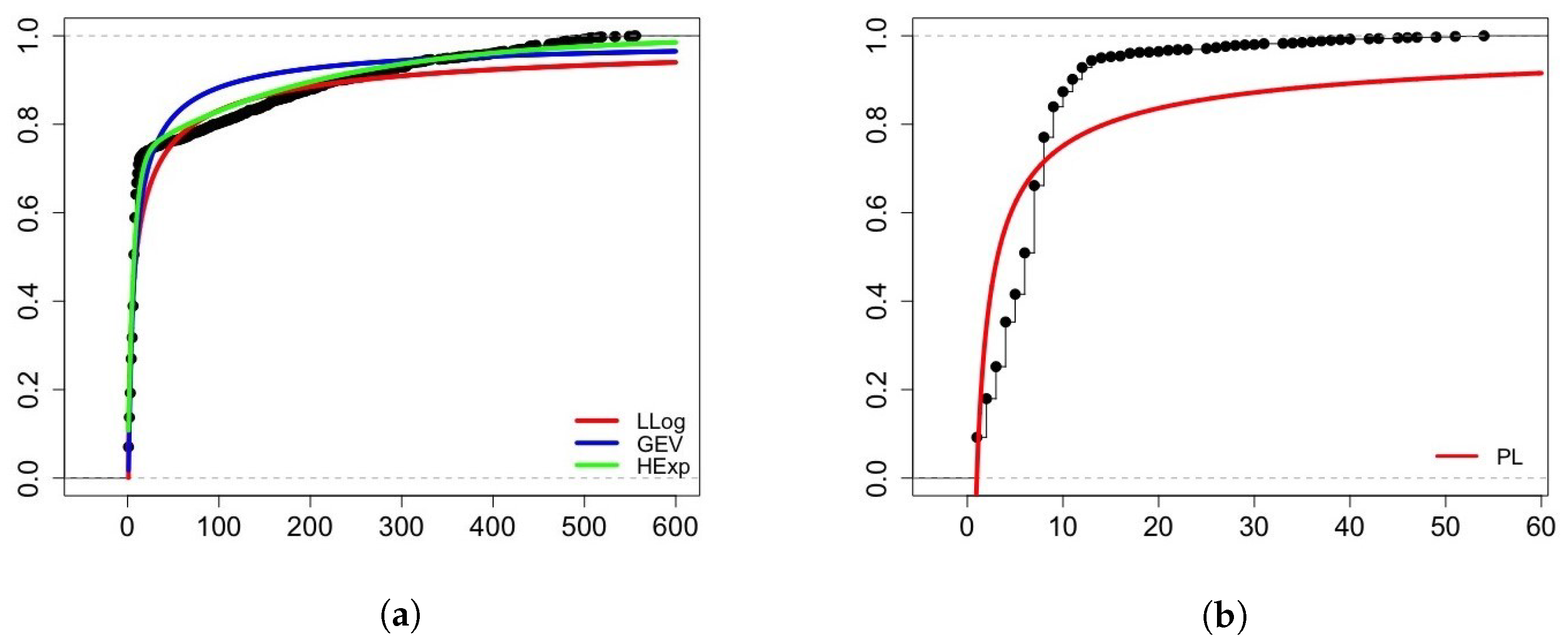
Figure 12 shows the EDF, comparing it with the investigated fits that are supported by at least one goodness-of-fit test. The power law case is shown again separately, with the lack of fit to the censored data being quite striking.

From the above results, the log-logistic and hyperexponential ($m=2$) are the two strongest candidates to model the data. If the choice were to be made solely based on AIC, the log-logistic would be selected. However, Figure 12a seems to reveal that the hyperexponential provides a more adequate fit, since it more closely follows the EDF towards the center to the right of the empirical data distribution. To better justify the choice between these two models, once again, the Vuong test can be helpful.

Comparing the log-logistic and hyperexponential ($m=2$) models, $L{R}_n=98.776$ (${\widehat{\omega }}_n=1.134$) and p-value = 0.023, and, therefore, there is some evidence in favor of the log-logistic having a better fit. Note, however, that if the decision is to be made using a significance level of 1%, the conclusion would be that there is some evidence (although weak) in favor of both models being equivalent.

6.2.2. Modeling the Data without Extreme Outliers

As mentioned earlier, the second modeling approach consists of considering a subsample of the 2022 sample without the extreme outliers (sample size $n=1553$). Statistics for this subsample are given in

Table 10. Statistics for the 2022 subsample.

Min	${\mathit{Q}}_1$	${\mathit{Q}}_2=\mathbf{Mode}$	Mean	${\mathit{Q}}_3$	Max	SD	Skewness	Kurtosis
1	4	7	11.3	9	111	18.89	3.53	12.04

, with some representations of the data being shown in Figure 13 (the bin width of the histogram is $h=7$ since all intervals have non-null frequencies).

The procedure described before to establish the power law signature was applied again to this subsample (see Figure 14). In this case, a linear signature is observed when $0<lnx<4$, or if $1<x<54.6$, with exactly the same condition obtained when working with the whole 2022 sample. Therefore, the results for the power law fit are identical in this context to those shown in Table 8, and for this reason will not be replicated here. The results for the other model fits are given in

Table 11. Parameters and goodness-of-fit results for some heavy-tailed models.

	KS	AD	CvM	AIC	BIC
Pareto
$\widehat{\alpha }=0.552\left(0.014\right)$	0.001	0.001	0.001	10,578.7	10,584.0
$\widehat{\delta }=1$	($D_n=0.297$)	($A_n^2=\infty$)	(${\omega }_n^2=1.811$)
Log-normal
$\widehat{\lambda }=1.811\left(0.025\right)$1	0.001	0.469	0.117	10,026.4	10,037.1
$\widehat{\delta }=0.997\left(0.018\right)$1	($D_n=0.141$)	($A_n^2=3.468$)	(${\omega }_n^2=0.939$)
Log-logistic
$\widehat{\alpha }=0.982\left(0.023\right)$	0.001	0.001	0.045	10,016.8	10,027.5
$\widehat{\lambda }=1$	($D_n=0.170$)	($A_n^2=9.905$)	(${\omega }_n^2=1.116$)
$\widehat{\delta }=4.510\left(0.188\right)$
General Extreme Value
$\widehat{\xi }=0.568\left(0.027\right)$	0.001	0.377	0.426	9946.2	9962.2
$\widehat{\lambda }=4.337\left(0.107\right)$	($D_n=0.{121}^{*}$)	($A_n^2=3.721$)	(${\omega }_n^2=0.676$)
$\widehat{\delta }=3.639\left(0.106\right)$
Generalized Pareto
$\widehat{\xi }=0.368\left(0.029\right)$	0.001	0.001	0.029	9353.5	9369.6
$\widehat{\lambda }=1$	($D_n=0.171$)	($A_n^2=\infty$)	(${\omega }_n^2=1.200$)
$\widehat{\delta }=6.856\left(0.258\right)$
Cauchy
$\widehat{\lambda }=6.102\left(0.100\right)$	0.001	0.091	0.509	10,297.1	10,307.8
$\widehat{\delta }=2.484\left(0.082\right)$	($D_n=0.130$)	($A_n^2=5.159$)	(${\omega }_n^2=0.633$)

¹ Estimates for the parameters of the logarithm of the random variable.

and

Table 12. Parameters and goodness-of-fit results for the hyperexponential model.

	KS	AD	CvM	AIC	BIC
$m=2$
${\tilde{\pi }}_1=0.890$; ${\tilde{\theta }}_1=0.158$	0.001	0.030	0.107	10,141.9	10,158.0
${\tilde{\pi }}_2=0.110$; ${\tilde{\theta }}_2=0.020$	($D_n=0.187$)	($A_n^2=6.243$)	(${\omega }_n^2=0.956$)
$m=3$
${\tilde{\pi }}_1=0.760$; ${\tilde{\theta }}_1=0.158$	0.001	0.030	0.107	10,145.9	10,172.7
${\tilde{\pi }}_2=0.130$; ${\tilde{\theta }}_2=0.158$	($D_n=0.187$)	($A_n^2=6.243$)	(${\omega }_n^2=0.956$)
${\tilde{\pi }}_3=0.110$; ${\tilde{\theta }}_3=0.020$

.

This modeling approach leads to some different conclusions from those when modeling with all the data. The log-normal, GEV, and Cauchy are potential model candidates, all being supported by both the AD and CvM tests. The hyperexponential is also a potential model candidate, but is only supported by the CvM test. Again there is no gain in using the hyperexponential $m=3$ model compared with the $m=2$ model. Curiously, the evidence in favor of the log-logistic model is no longer supported by any goodness-of-fit test, although the p-value of the CvM test is close to the significance level of 5%.

On the other hand, the GEV fit is the one that has the smallest AIC of all the fits, as well as the lowest value for the KS test statistic. Therefore, if the choice of a model is to be made solely on the AIC, the GEV model is clearly the winner, and the log-normal the runner up (it has the second smallest AIC). The different conclusions from the ones obtained before might be somewhat explained by the fact that the subsample used has a skewness of 3.53, as opposed to 2.29 for the whole sample, which introduces some changes in the characteristics of the data and, therefore, of the underlying data distribution.

Figure 15 displays the EDF, comparing it with the log-normal, GEV, Cauchy, and hyperexponential ($m=2$) fits. Observe that, despite the fact that the hyperexponential has the third lowest AIC of the four models, its fit again follows quite closely the EDF towards the center to the right of the empirical data distribution.

With the GEV and the log-normal models being the two strongest model candidates, it is advisable once again to use the Vuong test to support a choice. Comparing these two models, $L{R}_n=41.084$ (${\widehat{\omega }}_n=0.025$) and p-value = 0; hence, there is strong evidence in favor of GEV having a better fit here.

On the other hand, and out of curiosity, when comparing the GEV and hyperexponential ($m=2$) fits with the Vuong test, as $L{R}_n=97.879$ (${\widehat{\omega }}_n=0.120$), and the p-value $\approx 0$, when the choice is between GEV and the hyperexponential, the test’s results clearly suggest the first model. However, one must remember that the AIC (and the BIC) is an overall measure of goodness-of-fit, which may explain why a better fit is achieved with GEV.

The analysis of the number of days from publication to update of vulnerabilities using a systematic sample ($n=403$) from 2021 and a simple random sample ($n=1943$) from 2022 led to consistent results, both with respect to the basic sample statistics (Table 1, Table 2, Table 6, Table 7, and Table 10) and with respect to the choice of statistical models, with a clear indication that an extreme value (either GEV, in the classical setting of the maxima of IID random variables, or log-logistic in the context of geometrically thinned sequences of IID random variables, or a hyperexponential mixture of two exponential variables) provided the best fit.

Observe that to be on the safe side, the analysis was performed for the sets of all data and for the censored sets cleaned of extreme outliers, as indicated in the boxplot diagrams. But the adequacy of the hyperexponential fit seems to indicate that the data considered as outliers in the exploratory data analysis phase are data coming from the second component of the hyperexponential population.

There is some evidence, in view of the hyperexponential fit and of the sample statistics seen in Table 1, Table 2, Table 6, Table 7, and Table 10, that it is reasonable to split the data into two subsets at the three weeks threshold. This provides a naive indication of the weights of the first and second components of the hyperexponential fit, as shown in

Table 13. Weights for the hyperexponential fit (based on the 2022 sample).

Risk Level	Update-Publication $\le 21$	Update-Publication $>21$
Low	20 (86.96% )	3 (13.04%) $\approx \frac{1}{8}$
Medium	594 (77.55%)	172 (22.45%) $\approx \frac{1}{5}$
High	499 ( 67.43%)	241 (32.57%) $\approx \frac{1}{3}$
Critical	330 (79.71% )	84 (20.29%) $\approx \frac{1}{5}$
All	1443 (74.27%)	500 (25.73%) $\approx \frac{1}{4}$

.

A sensible conjecture is that hackers maintain interest in one-third of high-risk vulnerabilities during a longer period, while for medium-risk and critical-risk vulnerabilities (in this last case possibly because vendors prioritize patching investment and discourage hackers) only one-fifth have a long update period. With respect to low-risk vulnerabilities, the one-eighth of those taking a long update period is even smaller. Observe that there was a subsample of only 23 low-risk vulnerabilities, which seems negligible in a sample of size $n=1943$ (1.18%). The split sample statistics are indicated in

Table 14. Split sample statistics.

	Min	${\mathit{Q}}_1$	${\mathit{Q}}_2$	${\mathit{Q}}_3$	Max	Mean	SD
Medium Risk
Update-Publication ≤ 21	0	3	6	8	21	5.80	3.58
Update-Publication > 21	26	98.5	188	309	554	220.4	143.08
High Risk
Update-Publication ≤ 21	0	3	6	8	21	5.96	3.60
Update-Publication > 21	22	108	190	303	556	214.50	134.83
Critical
Update-Publication ≤ 21	0	4	6	8	19	6.27	3.39
Update-Publication > 21	27	92	180.5	331	505	217.3	144.19
All
Update-Publication ≤ 21	0	3	6	8	21	5.97	3.55
Update-Publication > 21	22	103.8	186	309	556	217.1	139.41

.

The close coincidence of values is striking. Concerning the quick update component, the median time is about one week, for the 3rd quartile, 8 days, and (although artificial) this slowly increases to the maximum time to update of 3 weeks.

With regard to the long updating vulnerabilities, around 25% of the vulnerabilities are updated up to 3 months, the median time to update is approximately 6 months, and the 3rd quartile is approximately 10 months.

This may inspire some ways of forecasting a dynamic CVSS score. Instead of the temporal metrics equation $\mathrm{TS}=\mathrm{RUp}\left(\mathrm{BS}\times \mathrm{ECM}\times \mathrm{RL}\times \mathrm{RC}\right)$ (see Appendix A and Section 2), a multiplier $R\left(t\right)$ can be used to obtain a time-dependent dynamic base score as

$$\mathrm{BS}\left(t\right)=\mathrm{RUp}\left(\mathrm{BS}\times R\left(t\right)\right),$$

where $R\left(t\right)$ is computed twice: for the fast updating component and for the slow updating component of the hyperexponential fit. This will necessarily produce two lines showing the probable evolution of the severity score of the vulnerability, assuming that the multiplier $R\left(t\right)$ appropriately reflects the behavior of hackers and vendors.

Adequate choices of the multiplier $R\left(t\right)$ depend on a fuller understanding of hackers’ behavior, and empirical evaluation must take into account its effect on the number of changes over time from medium to high, from high to critical, and vice versa, and, concomitantly, the time intervals in which these changes occur. These are informal indicators of the effectiveness of the R multipliers in boosting the CVSS.

An example, assuming that the interest of hackers in the vulnerability increases steadily until the 1st quartile and also between the 1st quartile and the median ($Q_2$), and that, in most cases, they will loose interest in the vulnerability (eventually, since the vendors invest in patching), is

$$R\left(t\right)=\left\{\begin{array}{cc}0,\hfill & t<0\hfill \\ 1+F^2\left(t\right),\hfill & 0\le t<Q_1\hfill \\ 1+0.{25}^2+\sqrt{\left[F\right(t)-0.25]F\left(t\right)},\hfill & Q_1\le t<Q_2\hfill \\ 1+0.{25}^2+\sqrt{0.25\times 0.5}+[F\left(t\right)-0.5][F\left(t\right)-0.75],\hfill & Q_2\le t<Q_3\hfill \\ 1+0.{25}^2+\sqrt{0.25\times 0.5}-(1+\sqrt{3})[F\left(t\right)-0.75],\hfill & Q_3\le t\hfill \end{array}\right..$$

Figure 16 exhibits the above multiplier function, as well as the evolution of a vulnerability with score 7.4 over time.

Although the initial aim of this research was to change the static status of the CVSS, the development of the work led to some reflections on the past and expected evolution of the measurement concept.

Just as the law of large numbers and the central limit theorem became non-physical measurement aids, and regression made it possible to measure one variable to evaluate another (for instance, an instrument to measure the glucose level on a daily basis explains in the technical description of the device that it effectively measures the angle of refraction of light in the blood deposited on the strip, and transforms this measurement into the “measurement” of glucose), the digital transition will eventually lead metrology to evolve towards encompassing other non-physical auxiliary means of measurement, such as metrics and CVSS indices and machine learning algorithms, such as those that evaluate EPSS (the theme of the 2022 World Metrology Day was ’Metrology in the Digital Era’).

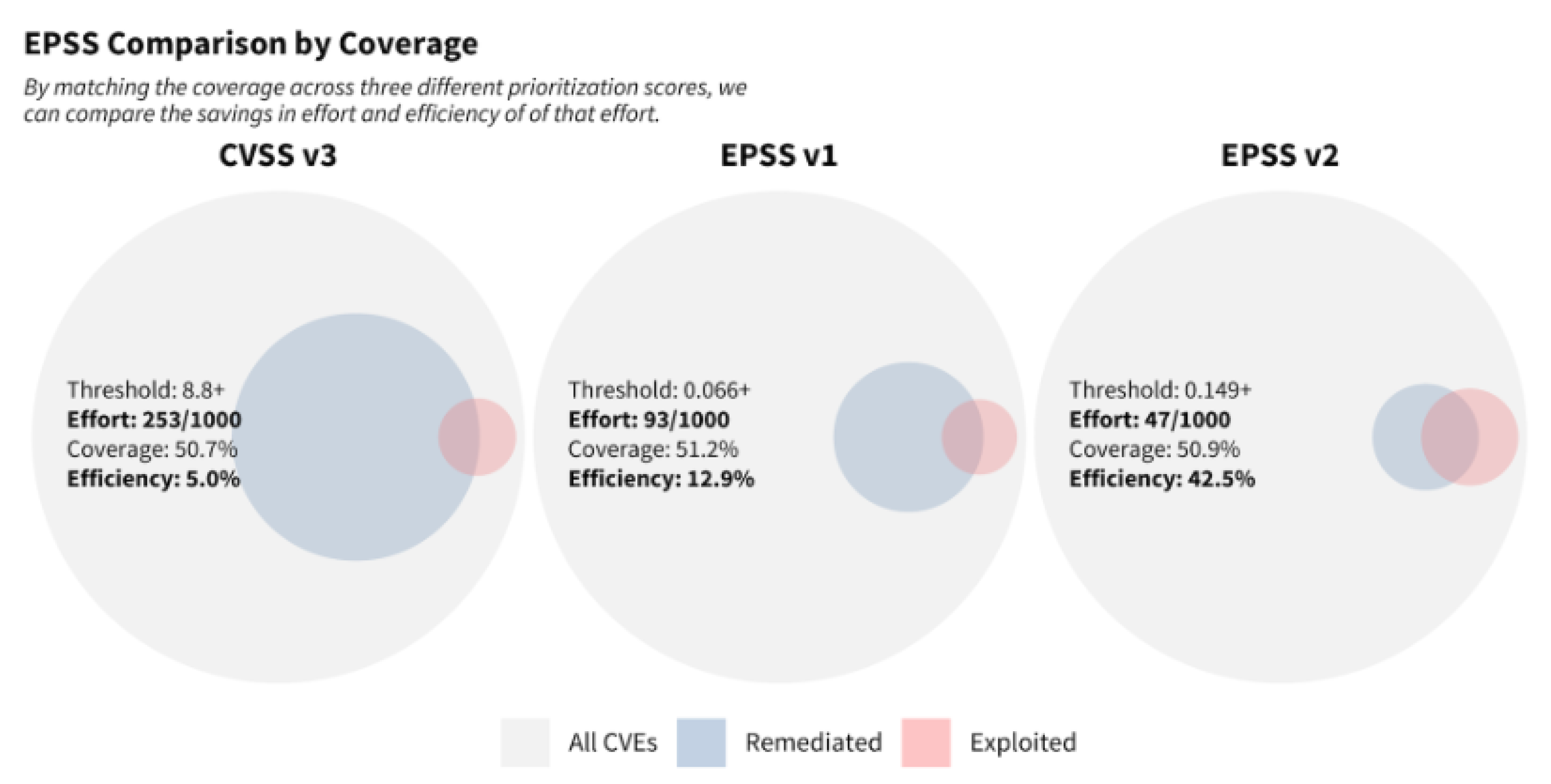
In the case of assessing the severity of vulnerabilities or the likelihood of risk of exploitation, it will imply hard work in the harmonization process and eventually a desirable evolution towards standardization. However, the situation is far from satisfactory. For example, with a file containing the vulnerabilities that in April 2021 to March 2022 were rated ’Functional’ or ’High’ with respect to the metric exploit code maturity (which is a collection of data, not a random sample), searching the CVE-ID in other databases to obtain CTI and EPSS, the unpleasant surprise was to find that the empirical correlations were $\mathrm{corr}(\mathrm{CVSS},\mathrm{CTI})=-0.12$, $\mathrm{corr}(\mathrm{CTI},\mathrm{EPSS})=-0.01$ and $\mathrm{corr}(\mathrm{CVSS},\mathrm{EPSS})=0.14$, indicating that they are uncorrelated scores. Thus, as prioritization guides in the urgency of patching vulnerabilities, while they are often concordant, they do not offer the comfortable sense of security to which such an economically sensitive area aspires.

7. Conclusions

Since the pathbreaking paper of Frei et al. [2], it has been common knowledge that accurate modeling inter-event times in the lifecycle of vulnerabilities is essential to assess the risk of exposure of a network. As Stumpf and Porter [53] highlighted, often the data available do not support the biased option of modeling using power laws. However, on the other hand, there exists sound evidence that heavy-tailed models should be used.

Therefore, the goodness-of-fit of competitive models, including Pareto, log-normal, log-logistic, general extreme value, generalized Pareto, and Cauchy, were investigated using the usual goodness-of-fit Kolmogorov–Smirnov, Anderson–Darling, and Cramér–von Mises tests, and the AIC and BIC. A refinement of statistical choice was obtained using Vuong’s test [11], with the overall conclusion that the GEV and log-logistic models provided the best adjustments. This is not surprising since the log-logistic is also an extreme value law in the context of geometrical thinning.

On the other hand, following the claim of Feldmann and Whitt [7] and Nurmi et al. [36] that hyperexponential models provide a good fit to long-tailed data, this was also investigated. The goodness-of-fit was striking, reflecting the fact that there is good reason to believe that attackers lose interest in most of the vulnerabilities quite soon, but some hackers maintain interest in some vulnerabilities for a long period. Thus the number of outliers in the samples of time from publication to the update of vulnerabilities indicates that very likely a mixture of at least two populations is present.

The number of yearly reported vulnerabilities has sharply increased since 2017, and this is the source of unavoidable limitations due to sampling. Another limitation comes from hackers’ diverse preferences for medium-, high-, and critical-risk vulnerabilities. However, the close coincidence of the sample statistics in Table 14 indicates some sort of stability.

As the thinned extreme value log-logistic law and the hyperexponential model provide such good fits to the data, the logical next step is to define a hyperlog-logistic model, combining the features of the two, and to implement the EM algorithm to compare the results.

References

1. CVSS. Common Vulnerability Scoring System, Version 3.1. Available online: https://first.org/cvss/calculator/3.1 (accessed on 7 August 2023).
2. Frei, S.; May, M.; Fiedler, U.; Plattner, B. Large-scale vulnerability analysis. In Proceedings of the 2006 SIGCOMM Workshop on Large-Scale Attack Defense, ACM, Pisa, Italy, 11–15 September 2006; pp. 131–138. [Google Scholar]
3. Holm, H. A large-scale study of the time required to compromise a computer system. IEEE Trans. Dependable Secur. Comput. 2013, 11, 2–15. [Google Scholar] [CrossRef]
4. Allodi, L. The heavy tails of vulnerability exploitation. In Engineering Secure Software and Systems, ESSoS 2015. Lecture Notes in Computer Science 8978; Piessens, F., Caballero, J., Bielova, N., Eds.; Springer: Berlin, Germany, 2015. [Google Scholar]
5. Ruohonen, J. A look at the time delays in CVSS vulnerability scoring. Appl. Comput. Inform. 2019, 15, 129–135. [Google Scholar] [CrossRef]
6. Rachev, S.T.; Resnick, S. Max-geometric infinite divisibility and stability. Stoch. Model. 1991, 7, 191–218. [Google Scholar] [CrossRef]
7. Feldmann, A.; Whitt, W. Fitting mixtures of exponentials to long-tail distributions to analyze network performance models. Perform. Eval. 1998, 31, 245–279. [Google Scholar] [CrossRef]
8. CVEdetails. Available online: https://www.cvedetails.com/ (accessed on 1 August 2023).
9. Akaike, H. Factor analysis and AIC. Psychometrika 1987, 52, 317–332. [Google Scholar] [CrossRef]
10. Schwarz, G.E. Estimating the dimension of a model. Ann. Stat. 1978, 6, 461–464. [Google Scholar] [CrossRef]
11. Vuong, Q.H. Likelihood ratio tests for model selection and non-nested hypotheses. Econometrica 1989, 57, 307–333. [Google Scholar] [CrossRef]
12. Tunggal, A.T. What is a Vulnerability? Definition + Examples, 2022. Available online: https://www.upguard.com/blog/vulnerability (accessed on 1 August 2023).
13. Eling, M.; Elvedi, M.; Falco, G. The economic impact of extreme cyber risk scenarios. N. Am. Actuar. J. 2022, 27, 429–443. [Google Scholar] [CrossRef]
14. Vulnerability Database. Available online: https://vuldb.com/ (accessed on 7 August 2023).
15. National Vulnerability Database. Available online: https://nvd.nist.gov/general/nvd-dashboard (accessed on 7 August 2023).
16. Exploit Database. Available online: https://www.exploit-db.com (accessed on 7 August 2023).
17. Anderson, R. Why information security is hard — an economic perspective. In Proceedings of the 17th Annual Computer Security Applications Conference (ACSAC), New Orleans, LA, USA, 10–14 December 2001. [Google Scholar]
18. Bollinger, J. Economies of disclosure. SIGCAS Comput. Soc. 2004, 34, 1. [Google Scholar] [CrossRef]
19. Dubendorfer, T.; Wagner, A.; Plattner, B. An economic damage model for large-scale internet attacks. In Proceedings of the 13th IEEE International Workshops on Enabling Technologies: Infrastructure for Collaborative Enterprises (WETICE’04), Modena, Italy, 14–16 June 2004; pp. 223–228. [Google Scholar]
20. Kannan, K.; Telang, R. An economic analysis of market for software vulnerabilities. In Proceedings of the Third Workshop on the Economics of Information Security, Minneapolis, MN, USA, 13–14 May 2004. [Google Scholar]
21. Qualys Research Report Laws of Vulnerabilities 2005. Available online: http://www.qualys.com/docs/Laws-Report.pdf (accessed on 7 August 2023).
22. Anderson, R.; Moore, T. The economics of information security. Science 2006, 314, 610–613. [Google Scholar] [CrossRef]
23. Frei, S. Security Econometrics — The Dynamics of (In)security. Ph.D. Thesis, ETH ZURICH, Zurich, Switzerland, 2009. [Google Scholar]
24. EPSS—Exploit Prediction Scoring System. Available online: https://www.first.org/epss/model (accessed on 7 August 2023).
25. Jacobs, J.; Romanosky, S.; Edwards, B.; Roytman, M.; Adjerid, I. Exploit Prediction Scoring System (EPSS). Digit. Threat. Res. Pract. 2021, 2, 1–17. [Google Scholar] [CrossRef]
26. CTI—Cyber Threat Intelligence. Available online: https://fidelissecurity.com/resources/edu/cyber-threat-intelligence/ (accessed on 7 August 2023).
27. CWSS—Common Weakness Scoring System. Available online: https://cwe.mitre.org/index.html (accessed on 7 August 2023).
28. SSVC—Stakeholder-Specific Vulnerability Categorization system. Available online: https://www.cisa.gov/stakeholder-specific-vulnerability-categorization-ssvc (accessed on 7 August 2023).
29. Frühwirth, C.; Männistö, T. Improving CVSS-based vulnerability prioritization and response with context information. In Proceedings of the 3rd International Symposium on Empirical Software Engineering and Measurement, Lake Buena Vista, FL, USA, 15–16 October 2009; pp. 535–544. Available online: https://ieeexplore.ieee.org/abstract/document/5314230 (accessed on 1 August 2023). [CrossRef]
30. Frei, S. Vulnerability Management. Master’s Thesis, Department of Management Technology and Economics, ETH ZURICH, Zurich, Switzerland, 2007. [Google Scholar]
31. Shahzad, M.; Shafiq, M.Z.; Liu, A.X. A large scale exploratory analysis of software vulnerability life cycles. In Proceedings of the 34th International Conference on Software Engineering, Zurich, Switzerland, 2–9 June 2012; pp. 771–781. [Google Scholar]
32. CVE—Common Vulnerabilities and Exposures. Available online: http://cve.mitre.org/cve/ (accessed on 7 August 2023).
33. Boechat, F.; Ribas, G.; Senos, L.; Bicudo, M.; Nogueira, M.; Aguiar, L.; Menasché, D. Is vulnerability report confidence redundant? Pitfalls using temporal risk scores. IEEE Secur. Priv. 2021, 19, 44–53. [Google Scholar] [CrossRef]
34. Wilk, M.B.; Gnanadesikan, R. Probability plotting methods for the analysis of data. Biometrika 1968, 55, 1–17. [Google Scholar] [CrossRef] [PubMed]
35. Burnham, K.; Anderson, D. Model Selection and Multimodel Inference: A Practical Information—Theoretic Approach; Springer: New York, NY, USA, 2002. [Google Scholar]
36. Nurmi, D.; Brevik, J.; Wolski, R. Modeling machine availability in enterprise and wide-area distributed computing environments. In Euro-Par 2005 Parallel Processing, Lecture Notes in Computer Science; Cunha, J., Medeiros, P., Eds.; Springer: Berlin, Germany, 2005; Volume 3648, pp. 432–441. [Google Scholar]
37. Symantec. Available online: https://www.symantec.com/ (accessed on 7 August 2023).
38. Aaberge, R. Gini’s nuclear family. J. Econ. Inequal. 2007, 5, 305–322. [Google Scholar] [CrossRef]
39. Clauset, A.; Shalizi, C.R.; Newman, M.E.J. Power-law distributions in empirical data. SIAM Rev. 2009, 51, 661–703. [Google Scholar] [CrossRef]
40. Schroeder, M. Fractals, Chaos, Power Laws: Minutes from an Infinite Paradise; Reedition Dover Publications: Mineola, NY, USA; Freeman: New York, NY, USA, 2009. [Google Scholar]
41. Sornette, D. Critical Phenomena in Natural Sciences: Chaos, Fractals, Self-organization and Disorder: Concepts and Tools, 2nd ed.; Springer Series in Synergetics; Springer: Heidelberg, Germany, 2006. [Google Scholar]
42. Newman, M.E.J. Power laws, Pareto distributions and Zipf’s law. Contemp. Phys. 2005, 46, 323–351. [Google Scholar] [CrossRef]
43. Belevitch, V. On the statistical laws of linguistic distributions. Ann. Soc. Sci. Bruxelles Ser. I 1959, 73, 310–326. [Google Scholar]
44. Mitzenmacher, M. A brief history of generative models for power law and lognormal distributions. Internet Math. 2004, 1, 226–251. [Google Scholar] [CrossRef]
45. Bee, M. On discriminating between lognormal and Pareto tail: An unsupervised mixture-based approach. Adv. Data Anal. Classif. 2022, 1–9. [Google Scholar] [CrossRef]
46. Karamata, J. Sur un mode de croissance régulière des fonctions. Mathematica 1930, 4, 38–53. [Google Scholar]
47. Feller, W. An Introduction to Probability Theory and its Applications, 2nd ed.; Wiley: New York, NY, USA, 1971; Volume 2. [Google Scholar]
48. Kevei, P. Regularly Varying Functions. 2019. Available online: https://www.math.u-szeged.hu/~kevei/tanitas/1819regvar/RegVar_notes.pdf (accessed on 1 August 2023).
49. Bingham, N.H.; Goldie, C.M.; Teugels, J.L. Regular Variation; Cambridge University Press: Cambridge, UK, 1989. [Google Scholar]
50. Hall, P. On some simple estimates of an exponent of regular variation. J. R. Stat. Soc. Ser. B 1982, 44, 37–42. [Google Scholar] [CrossRef]
51. Davis, R.; Resnick, S. Tail estimates motivated by extreme value theory. Ann. Stat. 1984, 12, 1467–1487. [Google Scholar] [CrossRef]
52. Fedotenkov, I. A review of more than one hundred Pareto-tail index estimators. Statistica 2020, 80, 245–299. [Google Scholar] [CrossRef]
53. Stumpf, M.P.H.; Porter, M.A. Critical truths about power laws. Science 2012, 335, 665–666. [Google Scholar] [CrossRef] [PubMed]
54. The Econophysics Blog. Tyranny of the Power Law (and Why We Should Become Eclectic). 2006. Available online: http://econophysics.blogspot.com/2006/07/tyranny-of-power-law-and-why-we-should.html (accessed on 1 August 2023).
55. Shalizi, C.R. So You Think You Have a Power Law? Well Isn’t that Special? 2007. Available online: bactra.org/weblog/491.html (accessed on 1 August 2023).
56. Box, G.E.P. Robustness in the strategy of scientific model building. In Robustness in Statistics; Launer, R.L., Wilkinson, G.N., Eds.; Academic Press: Cambridge, MA, USA, 1979; pp. 201–236. [Google Scholar]
57. Arnold, B.C. Pareto Distributions, 2nd ed.; Chapman and Hall/CRC: New York, NY, USA, 2015. [Google Scholar]
58. Embrechts, P.; Klüppelberg, C.; Mikosch, T. Modelling Extremal Events for Insurance and Finance; Springer Science & Business Media: Berlin, Germany, 1997; Volume 33. [Google Scholar]
59. Andriani, P.; McKelvey, B. Beyond Gaussian averages: Redirecting international business and management research toward extreme events and power laws. J. Int. Bus. 2007, 38, 1212–1230. [Google Scholar] [CrossRef]
60. Johnson, N.L.; Kotz, S.; Balakrishnan, N. Continuous Univariate Distributions, 2nd ed.; Wiley: New York, NY, USA, 1994; Volume 1. [Google Scholar]
61. Beirlant, J.; Teugels, J.L.; Vynckier, P. Practical Analysis of Extreme Values; Leuven University Press: Leuven, Belgium, 1996. [Google Scholar]
62. Gomes, M.I.; Guillou, A. Extreme value theory and statistics of univariate extremes: A review. Int. Stat. Rev. 2015, 83, 263–292. [Google Scholar] [CrossRef]
63. Cline, D. Convolution tails, product tails and domains of attraction. Probab. Theor. 1986, 72, 529–557. [Google Scholar] [CrossRef]
64. Malik, H.J. Estimation of the parameters of the Pareto distribution. Metrika 1970, 15, 126–132. [Google Scholar] [CrossRef]
65. Bauke, H. Parameter estimation for power-law distributions by maximum likelihood methods. Eur. Phys. J. B 2007, 58, 167–173. [Google Scholar] [CrossRef]
66. Diaz, F.J. Identifying tail behavior by means of residual quantile functions. J. Comput. Graph. Stat. 1999, 8, 493–509. [Google Scholar] [CrossRef]
67. Arnold, B.C.; Brockett, P.L. When does the βth percentile residual life function determine the distribution? Oper. Res. 1983, 31, 391–396. [Google Scholar] [CrossRef]
68. Davison, A.C.; Hinkley, D.V. Bootstrap Methods and their Application; Cambridge University Press: Cambridge, UK, 1997. [Google Scholar]
69. Glaz, J.; Sison, C.P. Simultaneous confidence intervals for multinomial proportions. J. Stat. Plan. Inference 1999, 82, 251–262. [Google Scholar] [CrossRef]
70. Dugal, D.; Rich, D. Announcing CVSSv4.0. In Proceedings of the 35th Annual FIRST Conference, Montréal, QC, Canada, 4–9 June 2023. [Google Scholar]
71. Johnson, N.L.; Kotz, S.; Kemp, A.W. Univariate Discrete Distributions, 2nd ed.; Wiley: New York, NY, USA, 1992. [Google Scholar]
72. Saichev, A.; Malevergne, Y.; Sornette, D. Theory of Zipf’s law and beyond. In Lect. Notes Econ. Math. Systems; Springer: Berlin, Germany, 2010; Volume 632. [Google Scholar]
Figure 1. Monthly registered vulnerabilities (source: https://first.org/epss/data_stats (accessed on 7 August 2023). Copyright © 2023 Forum of Incident Response and Security Teams, Inc. All Rights Reserved).
Appliedmath 04 00002 g001
Figure 2. Efficiency of CVSS and EPSS (source: https://www.first.org/epss/model (accessed on 1 September 2023) Copyright © 2023 Forum of Incident Response and Security Teams, Inc. All Rights Reserved).
Appliedmath 04 00002 g002
Figure 3. Vulnerabilitieslifecycle (source: Frei et al. [2]).
Appliedmath 04 00002 g003
Figure 4. Representations of the 2021 sample: (a) Frequency histogram. (b) Boxplot. (c) Empirical distribution function.
Appliedmath 04 00002 g004
Figure 5. Power law linear signature in a log-log plot (2021 sample).
Appliedmath 04 00002 g005
Figure 6. Representations of the 2021 censored sample: (a) Frequency histogram ( h = 7 ). (b) Boxplot. (c) Empirical distribution function.
Appliedmath 04 00002 g006
Figure 7. Empirical distribution function (black line) and fitted models: (a) Pareto (Par), log-normal (LN), log-logistic (LLog), general extreme value (GEV), generalized Pareto (GP), and hyperexponential m = 2 (HExp). (b) Power law (PL).
Appliedmath 04 00002 g007
Figure 8. Representation of the CVSS base score sample.
Appliedmath 04 00002 g008
Figure 9. Representations of the 2022 sample: (a) Frequency histogram. (b) Boxplot. (c) Empirical distribution function.
Appliedmath 04 00002 g009
Figure 10. Power law linear signature in a log-log plot (2022 sample).
Appliedmath 04 00002 g010
Figure 11. Representations of the 2022 censored sample: (a) Frequency histogram ( h = 7 ). (b) Boxplot. (c) Empirical distribution function.
Appliedmath 04 00002 g011
Figure 12. Empirical distribution function (black line) and fitted models: (a) log-logistic (LLog), general extreme value (GEV), and hyperexponential m = 2 (HExp). (b) Power law (PL).
Appliedmath 04 00002 g012
Figure 13. Representations of the 2022 subsample: (a) Frequency histogram. (b) Boxplot. (c) Empirical distribution function.
Appliedmath 04 00002 g013
Figure 14. Powerlaw linear signature for the 2022 subsample in a log-log plot.
Appliedmath 04 00002 g014
Figure 15. Empirical distribution function (black line) and fitted models: log-normal (LN), general extreme value (GEV), Cauchy (Cau), and hyperexponential m = 2 (HExp).
Appliedmath 04 00002 g015
Figure 16. (a) Multiplier R ( t ) . (b) Evolution of score 7.4 over time assuming the multiplier R ( t ) .
Appliedmath 04 00002 g016