Article

Exploring Price Patterns of Vegetables with Recurrence Quantification Analysis

by
Sofia Karakasidou
1,*,
Athanasios Fragkou
2,
Loukas Zachilas
1 and
Theodoros Karakasidis
3
1
Department of Economics, University of Thessaly, 38334 Volos, Greece
2
Department of Civil Engineering, University of Thessaly, 38334 Volos, Greece
3
Department of Physics, University of Thessaly, 35100 Lamia, Greece
*
Author to whom correspondence should be addressed.
AppliedMath 2024, 4(3), 1012-1046; https://doi.org/10.3390/appliedmath4030055
Submission received: 22 July 2024 / Revised: 15 August 2024 / Accepted: 22 August 2024 / Published: 26 August 2024

Abstract

:
This study investigates the time-series behavior of vegetable prices in the Central Market of Thessaloniki, Greece, using Recurrence Plot (RP) analysis and Recurrence Quantification Analysis (RQA), which considers non-linearities and does not necessitate stationarity of time series. The period of study was 1999–2016 for practical and research reasons. In the present work, we focus on vegetables available throughout the year, exploring the dynamics and interrelationships between their prices to avoid missing data. The study applies RP visual inspection classification, a clustering based on RQA parameters, and a classification based on the RQA analysis graphs with epochs for the first time. The aim of the paper was to investigate the grouping of products based on their price dynamical behavior. The results show that the formed groups present similarities related to their use as dishes and their way of cultivation, which apparently affect the price dynamics. The results offer insights into market behaviors, helping to inform better management strategies and policymaking and offer a possibility to predict variability of prices. This information can interest government policies in various directions, such as what products to develop for greater stability, identity for fluctuating prices, etc. In future work, a larger dataset including missing data could be included, as well as a machine-learning algorithm to classify the products based on the RQA with epochs graphs.

1. Introduction

Vegetable prices significantly impact both the economy and consumers’ daily lives. Thus, there is increasing interest in an extensive and macro-level study of vegetable price research, as can be seen from several medical and societal works [1,2], which have shown that the consumption of fruit and vegetables is low worldwide, particularly in low-income countries and conclude that policies worldwide should enhance the availability and affordability of such products. Similar results were obtained in [3] in which pricing effects on food choices have been studied. In [4], the authors investigated if price is a barrier to fruit and vegetable consumption for low-income families by comparing the average cost of a market basket of fruits and vegetables.
Many aspects have been investigated in the literature since prices are affected by a series of factors. The interest in the subject has also attracted bibliometric research in order to find interest in countries (see, e.g., [5]). In that study [5], by sorting out a large volume of documents, a visual representation of the vegetable price research literature is presented for vegetable prices hot issues, and it clearly shows the focus of the research on the fluctuation pattern of vegetable prices, analyses of the influencing factors of vegetable price fluctuation among other findings. Here, we focus on representative papers from the literature (some more recent than paper [5]) that explored several aspects of prices.
There is interest in the effect of the prices from several external factors. Researchers have analyzed vegetable prices by considering influencing factors, focusing on particular regions and vegetable varieties. Several studies have explored the effect of petroleum prices on vegetable prices [6,7,8,9] as well as the effect of coal prices [10] since energy is necessary in running the agricultural machinery as well as required to maintain given conditions for growth as is the case for greenhouses, as well as transportation of goods towards the markets, to mention a few examples.
An economic factor that several researchers have explored was exchange rates [7] since these factors affect several aspects from imported goods necessary for agriculture as well as the pricing for exported or imported vegetables since they also affect other parameters like energy or materials needed for cultivation, along with the competitiveness of the prices in an internationally open market.
The effect of weather has been investigated in some cases, for example [11]. This study took pointed pepper, loofah, Chinese chives, and tomato as examples, using weekly wholesale prices and corresponding weather factors data from one of the leading production areas in China based on the vector autoregressive (VAR) and the time-varying parameter vector autoregressive (TVP-VAR) models to explore the dynamic impacts of weather changes on vegetable price fluctuations. It was found that price fluctuations of specific vegetable varieties were affected by changes in particular weather factors. The shock intensity of weather factor changes in the same lag period on the current vegetable price fluctuations was time-varying, which could describe the historical dynamics of the impacts of weather changes on vegetable price fluctuations. Vegetable price fluctuations were primarily affected by their own lag periods, and the shock intensity of vegetable price fluctuations with equal lag periods on their own current price fluctuations was relatively stable. The dynamic impacts of vegetable price fluctuations occurring at chosen time points on its own later fluctuations were highly consistent in the variation from the beginning of the most substantial positive shock to the final dissipation.
Other researchers have employed models constructed by demand, supply, import, and export functions to decompose price variance and also performed simulations to generalize the results, for example, in the Korean vegetable market and selected cabbage, radish, dried red pepper, garlic, and onion as research objects [12]. The results indicate that the variability of domestic production is the primary factor influencing price fluctuations in the Korean vegetable market. The analysis revealed that demand, import, and export had a limited impact on price fluctuations in the Korean vegetable market, except for dried red pepper and onions.
In another paper [13], the authors analyzed the price behavior and growth trend in the area, production, and productivity of onion in several Indian markets using time-series analysis for the study of the price behavior and the compound growth rate employed to study the area, production, and productivity of the onion. The analysis indicated that seasonality influenced the price behavior of onions but was not the sole factor, although there was an increasing trend. Ref. [14] motivated the rise of the price of vegetables in India after the post-2008 global food crisis. Focusing on onions, an essential constituent of the Indian diet, this paper aimed to explore the causes of high price volatility. Their findings include that despite markets being integrated and no significant climatic shocks to production, there exists a vital element of uncertainty in market arrivals of onions, pointing toward the market power immediately downstream the production or anti-competition trade practices in major markets as a cause of high price volatility. Finally, they propose measures to manage price volatility, such as an increase in minimum export prices and bans on exports, which are also not found to have an immediate cooling effect on prices.
Several studies employ prediction methodologies to assess price estimations. Such work is the one to predict wholesale prices in the case of China for 15 years since 2000 [15]. The authors analyze agricultural price fluctuation factors and design a least square Support Vector Regression (SVR) model to predict the wholesale agricultural product price. Another study uses the STL-LSTM Method to predict values [16]. This study developed a monthly price forecasting model for Chinese cabbages and radishes. It showed the importance of input variables when forecasting vegetable prices and confirmed that meteorological and research volume index data helped improve a forecasting model’s accuracy. When the proposed methods were used in this study, the monthly price forecast accuracies were 88.74% and 92.05%, respectively, for Chinese cabbages and radishes. The proposed model is expected to be used to autonomously adjust supply and demand and to develop relevant policies to save social costs on agricultural product yields.
The common part of many studies is time-series analysis, which is vital in understanding the system’s dynamics under study and predicting its behavior. Such methods have been applied successfully in various systems (physical, economic, biological, etc.). Most methodologies assume the linearity of the dynamical system’s behavior and the presence of stochastic noise and do not consider nonlinear dynamic effects. Well-known and widespread methods such as the autocorrelation function and power spectrum have proven remarkably successful in time-series analysis. However, these methods must be revised to analyze nonlinear deterministic systems as they fail to detect nonlinear correlations. In addition, the clustering technique contributes to the formation of groups of products based on common characteristics. Other methods consider the more complex and often nonlinear behavior of the systems, such as phase space methods recurrence plots and time-series transformed complex networks, to mention a few examples. Recurrence Plots have been applied with success in various areas, such as wind power forecasting [17] in the analysis of molecular simulations [18], EEG analysis [19], financial data [20], and magnetohydrodynamic flows [21]. Hierarchical clustering allows us to divide items into categories without placing a priori restrictions on the number of groups into which our data are separated [22]. In many cases, combining the results of such analyses and performing a clustering based on them leads to a good categorization that considers several dynamic aspects of the system. An advantage also of the methodology is that the time series under study does not need to be stationary as is the case, for example, in the study of autocorrelation or other methods, and thus can directly employ the time series and is the methodology we employ in the present study for the first time.
From a general point of view, all the above kinds of studies, i.e., understanding the dynamics of prices and/or predictions, can play an essential role in managing central markets and policies concerning vegetable consumption and prices. Identifying common dynamic behavior between different vegetables, especially those of large consumption, is necessary. Understanding the dynamics of the process can help to see if there are any categories of products that form groups and could also see how one can classify products for market decisions or combined movement of prices due to their use and other parameters, such as external factors, for example, extended use of greenhouses, etc. This can be used in several ways to study individual dynamics and correlations. There is not to our knowledge a study concerning the grouping of products based on their price dynamical behavior and an investigation if the behavior is related to the use of the products as dishes as well as to their way of cultivation (in the field, in greenhouses, combined).
This work aims to study the price evolution in the time of several vegetables in a central market to identify dynamics of the price variation as well as similarities in behavior and relate them to characteristics of the products and their use without a priori assumptions. A central market is where producers’ products are concentrated or by large buyers and then resold to various shops. Thus, these prices are more closely related to the retail prices that customers must pay. For this aim, we have chosen the price of vegetables in the Thessaloniki Central Market as a case study. The Central Market of Thessaloniki (C.M.TH. S.A.) is a Société Anonyme with the sole shareholder being the Hellenic Corporation of Assets and Participations (HCAP) and is supervised by the Ministry of Development and Investment. It is the second largest central market in Greece after Athens in the case of Greece and products from this market travel quite large distances ranging from Thessaloniki, the second largest city of Greece, to many regions in northern Greece.
In the present paper, we extended the work using several methods to classify the products using a large time series of given vegetables. We focus on the study of price dynamics as they are formed not at the producer level but at the buyers for reselling or use in restaurants, etc., and reseller shops. To our knowledge, there is no such study existing. The aim is to identify if it is possible from the time-series dynamics to classify the products into categories/groups that will reveal a co-movement of process and determine the existence of characteristic times of the system based on nonlinear methods. It is the first time such an analysis with RP and RQA with epochs is performed in the literature. This classification can be employed in the future for all the products without any prior assumption and reveal groups of products that behave similarly. The results can be used to identify groups of products with similar dynamic behavior and can be employed in policies of buying and selling products from central markets, independent buyers, and the people who cultivate the products. This information can interest government policies in various directions, such as what products to develop for greater stability, identity for fluctuating prices, etc.
The structure of the paper is as follows. In Section 1, we present a literature review along with a focus on the problem studies in the present paper. In Section 2, we present the data employed in the present work along with the methodology concerning Recurrence plots, recurrence quantification analysis, and analysis with epochs. We must mention that these methods are applied for the first time in such data. In Section 3, the results are presented, and the possible relations between different types of products (vegetables) are discussed, trying to explain also based on their use. Finally, the conclusions are presented in Section 4.

2. Methodology

2.1. Recurrence Plots

Recurrence Plot is a graphical tool introduced by Eckman et al. [23] to extract qualitative information on a dynamical system through the study of its time series. One of its advantages is that it can be applied to non-stationary data. The first step in constructing a recurrence plot is to reconstruct phase space from the time series. The phase space is a representation of the dynamical system with all the states that can be “visited” by the system depending on its number of state variables (system dimensionality). It also has the advantage that the time is not explicitly presented. In general, we do not know the exact phase space of the system, but there is a methodology of delay for the reconstruction of the system state from the time series of the system [24,25]. The state vectors x i are constructed using in the following way x i = [ x ( t i m 1 τ d ) ,   x t i m 2 τ d ) , , x t i   ( τ d is the estimated time lag, the distance between time-series points that are employed in the procedure and m is the so-called embedding dimension of the system).
For the phase space reconstruction, we first estimate the time lag for the embedding. Fraser and Swinney [26] suggested the Average Mutual Information Equation (1) to choose the appropriate time lag, with the main advantage being compared with the autocorrelation function, which takes into account nonlinear correlations.
I = i j N p i j t l n p i j t p i t p j t    
where p i ( t ) is the probability of the i-interval as a value of the time series, and p i j ( t ) is the joint probability of the i-th interval as an observation, then in the j-th interval is an observation in later time τ. Fraser and Swinney report that if, at a point in time τd, the average mutual information falls at its first minimum value, then this time lag is a reasonable choice of the proper time delay for estimating the embedding dimension. Taking this lag into account, False Nearest Neighbors is a method by which one can estimate the optimal embedding dimension m by observing for false neighbors in the phase space [27].
In the next step, we embed the time series, forming a sequence of vectors x i = [ x ( t i m 1 τ d ) ,   x t i m 2 τ d ) , , x t i ( τ d is the estimated time lag), and then we calculate distances d i , j = x i x j between points i , j in the m-dimensional reconstructed phase space. A matrix of distances called a recurrence matrix is constructed then according to Equation (2)
R i , j = Θ ε ι x i x j , x i R m , i , j = 1,2 , . , N
where R i , j is the recurrence matrix, m is the embedding dimension, ε the cutoff distance for the points considered to be recurrent, and Θ is the Heaviside function. The Heaviside function takes a value equal to 1 when the points are located at smaller distances than the cutoff distance ε; otherwise, Θ = 0 (points are located at bigger distances than the cutoff distance ε). On the texture of a Recurrence plot, a black dot is placed at coordinates ( i , j ) if R i , j = 1 and a white dot if R i , j = 0 . Recurrence Plots are symmetric with respect to the main diagonal ( R i , i = 1 ). When computing an RP, a norm must be chosen. In the present study, the Euclidean norm was used. Each point in the phase space represents a state of the corresponding dynamical system, and the embedding parameters indicate the number of parameters/variables that affect the system (dimensionality m).
Recurrence Plot structure mainly contains lines parallel to the main diagonal (a sign of deterministic processes), white regions (abrupt changes in the dynamics of the system), and isolated points (strong fluctuations). Recurrence plots of deterministic processes may contain big diagonal lines, in contrast to Recurrence Plots of strongly fluctuating processes containing single isolated points. Diagonal lines indicate that successive states (i, j), (i + 1, j + 1), …, (i + l, j + l) (l = the length of the diagonal line) are recurrent, indicating the existence of a deterministic low behind such an evolution. A stochastic system forms only scattered points or very small lines and does not present any specific structure of the plot.
If, during the evolution of the system, there are states that are trapped in time, which means that they stay around a given state, then we observe then vertical and horizontal lines appear on the RP’s texture, forming black regions since states (i, j), (i, j + 1), …, (i, j + TT) or states (i, j), (i + 1, j), …, (i + TT, j) are located around a given state for TT time.
On the other hand, if we observe parallel diagonal lines (deterministic behavior), the distance between these lines corresponds to a characteristic system period. We can observe more than one frequency in several systems, such as annual periodicity, semester periodicity, etc.
We must mention here that an advantage that the RP analysis presents is that there is no need for the time series examined to be stationary compared to other methods like autocorrelation, Fourier transforms, etc., and that takes into account possible non-linearities existing in the system dynamics that are not taken into account by linear methods.

2.2. Recurrence Quantification Analysis

To quantify the visual information of the RPs, Zbilut and Webber [28] introduced several quantities, giving rise to the so-called Recurrence Quantification Analysis (RQA). These quantifiers count the black dots on the recurrence Plot and quantify the lines forming those dots (diagonal and vertical). We briefly present some of the RQA indices that have been proposed and use them for the present work:
  • %Recurrence or RR: the ratio of the number of recurrence points to the total number of points in the plot
R R = 1 N 2 i , j = 1 N R i , j     R i , j = 1 ,   i , j   r e c u r r e n t     0 ,   o t h e r w i s e
  • %Determinism or DET: The percentage of recurrence points which form diagonal lines:
D E T = l = l m i n N l P ( l ) l = 1 N l P ( l )
P(l) is the histogram of the lengths l of the diagonal lines.
The threshold is employed in order to exclude the diagonal lines formed by the tangential motion of the phase space trajectory [29], and this choice can also be such that one excludes short temporal scale correlations that can be ignored.
  • Average Diagonal Line Length, L: The average length of the diagonal line segments in the plot, excluding the main diagonal.
L = l = l m i n N l P ( l ) l = l m i n N P ( l )
  • Laminarity LAM: The percentage of recurrence points which form vertical lines:
L A M = v = v m i n N v P ( v ) v = 1 N v P ( v )
P(v) is the histogram of the lengths v of the vertical lines. Increased laminarity means that the system stays close to given states quite often. The trapping time quantifies the time the system stays close to a given state on average. A stochastic system represents very low laminarity.
  • Trapping Time, TT: It shows the average length of the vertical lines. Trapping Time represents the average time that the system has been trapped in the same state.
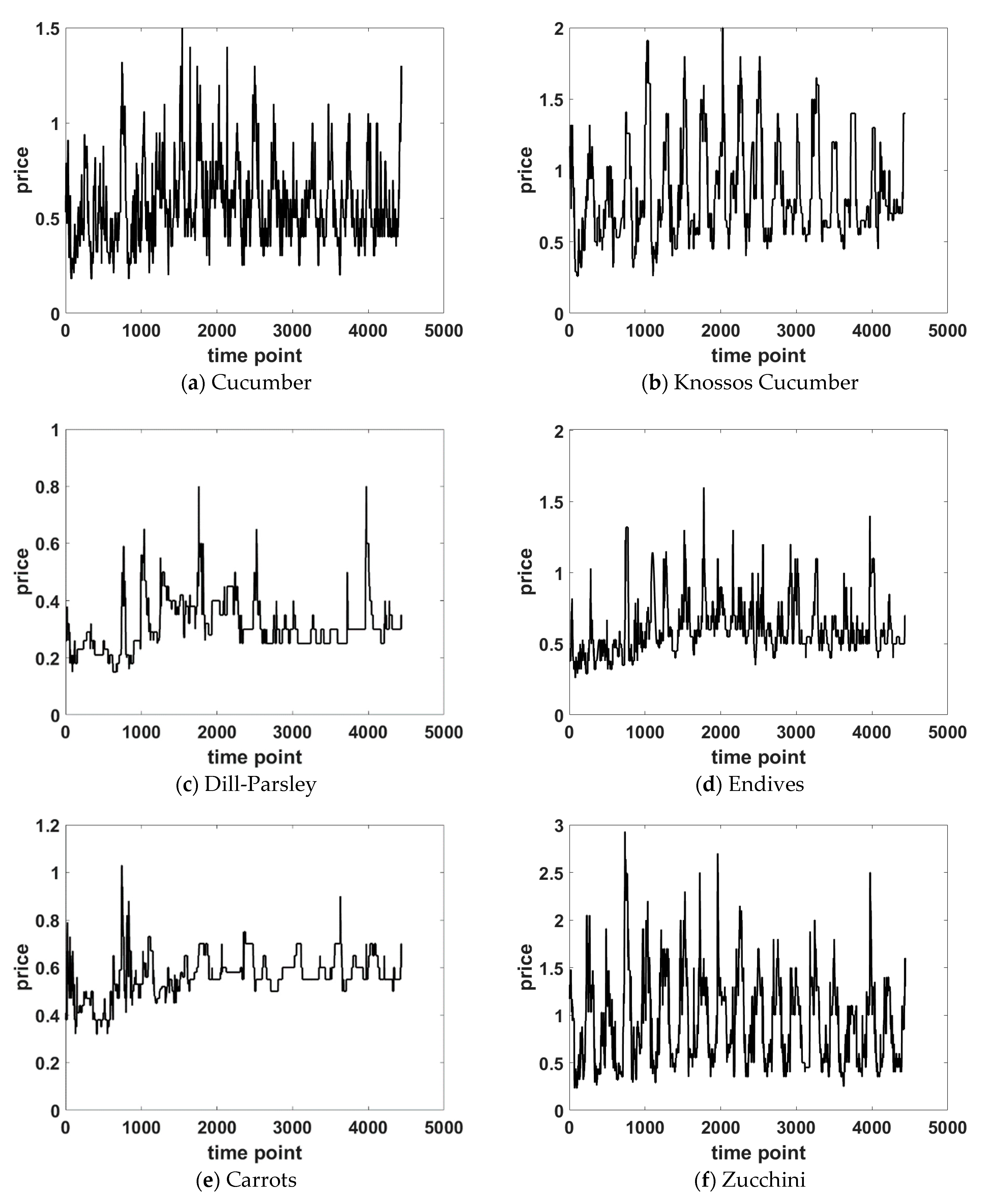
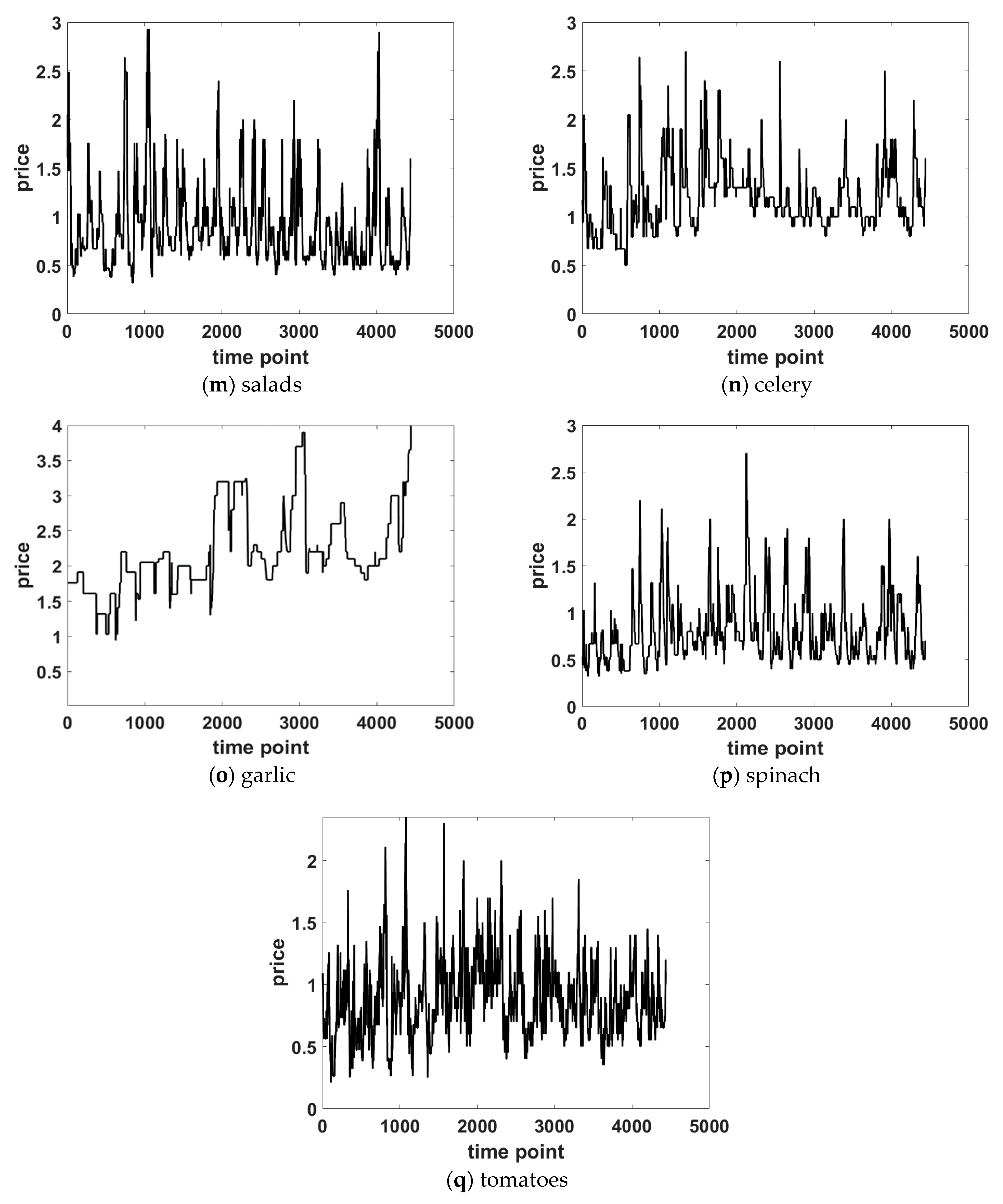
T T = υ = υ m i n N υ P ε ( υ ) υ = υ m i n N P ε ( υ )
It is evident from its definition that it is related to laminarity. Larger TT means that the system stays longer close to a given state. A stochastic system represents a very low TT compared to a deterministic one.
Moreover, we can observe large white regions, which correspond to abrupt changes in the dynamics of the system. White regions correspond to non-recurrent points. In many cases, diagonal lines are separated by white bands, which indicate perturbation (smaller or larger duration) due to an effect on the dynamical system.
For the calculation of the RPs and the RQA, we used the tool ‘Command line Recurrence plots’ [29] downloaded at [30] and CRP toolbox ver. 5.12, Release 25 (Marwan 2008) (for Recurrence Plots, RQA) [29] downloaded at [30]. For estimating time lag τ and embedding dimension m, we used the toolbox “Time-Series Analysis” (TI.SE.AN.) [31] downloaded at [32].
For further understanding, we applied the Recurrence Quantification Analysis with epochs to locate the time periods in which those changes took place. Epochs are equidistant time periods calculated along the main diagonal of the Recurrence plot, helping us to locate possible phase transitions during the evolution of the system. In fact, one performs the same analysis but over given sliding time windows to locate more subtle changes in the dynamics as a function of time. According to the method, transitions of the system are located by the visualization of the Recurrence Plots structure and delimiting regions with different textures (diagonal lines, white areas, or isolated points). Dissimilarities in structure between the located regions, along with the Recurrence Quantification Analysis, is a good indication of transitions between states of the system under study.

2.3. Data

The data originate from the Thessaloniki Central Market for the period 1999–2016. They were kept in handwritten form up until 2010, so they had to be entered manually and checked again. The remaining data existed in electronic format but were stored separately in files, requiring re-entry into the database and integrity checks. The entire dataset was checked for inconsistencies and errors. The values concern only working days.
The lower time limit (1999) is because we could not have access to the handwritten data before 1999. As far as the upper limit is concerned, we would like to avoid taking into account increased climate change effects [33,34] on one side and COVID-19 effects after December 2019 at the present state of the research. This will be investigated in future research.
Several series presented many periods of missing values, either due to seasonal but not systematic bookkeeping or weather effects like very low temperatures that have destroyed the production. Therefore, we decided to focus our study on time series that exhibited continuous data without any missing values. We specifically chose vegetables that demonstrated continuous values without any missing periods. The whole dataset concerns 17 products, as presented in Table 1.
In Figure 1, we present the time series of the selected products. We can see that several products exhibit periodic variation over time, such as Knossos Cucumber, Zucchini and Peppers. In some cases, this periodicity is quite clear, while in others, this variability is slightly modified or less evident. For example, this is the case with cucumber, spring onions, garlic, and tomatoes. We believe that this is because these products are primarily grown in greenhouses, which affects their price variability.
In the study, it was found that peppers have the highest price variation among all the products analyzed. Tomatoes display a somewhat periodic pattern in prices, but with more fluctuations, possibly because they are mainly used in salads and popular tourist dishes like “Greek salad”. They are also grown in large quantities in greenhouses, especially in Crete. Additionally, tomatoes are a popular salad ingredient, particularly before Easter, when people traditionally consume less meat.
Other products present more complex behavior such as beetroots and garlic. Salads (here correspond to red leaf lettuce and romaine lettuce) have smaller periodicities since their production has been enhanced with healthier food and increased cultivation. However, extreme weather conditions can significantly affect their production, raising prices.

3. Results

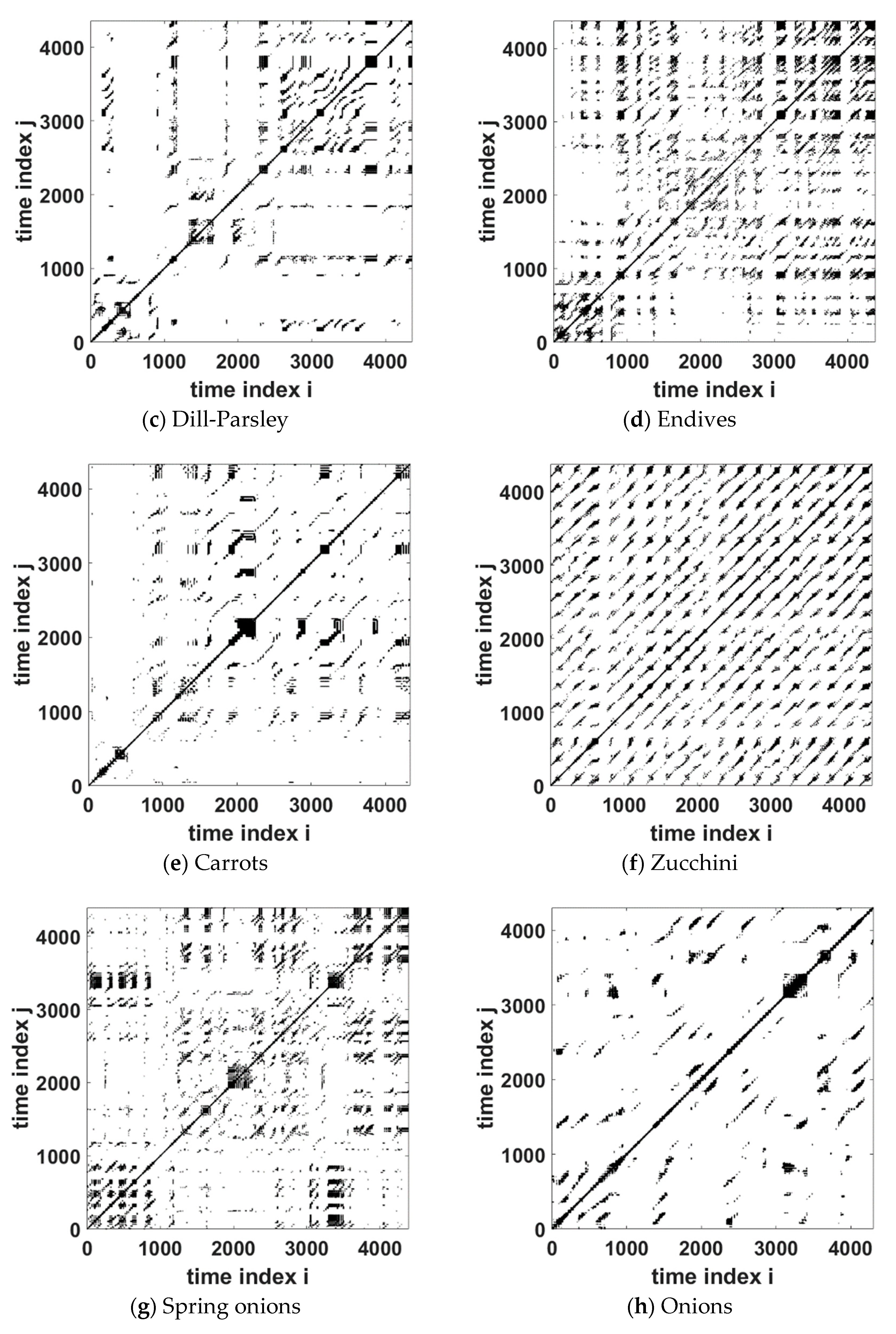
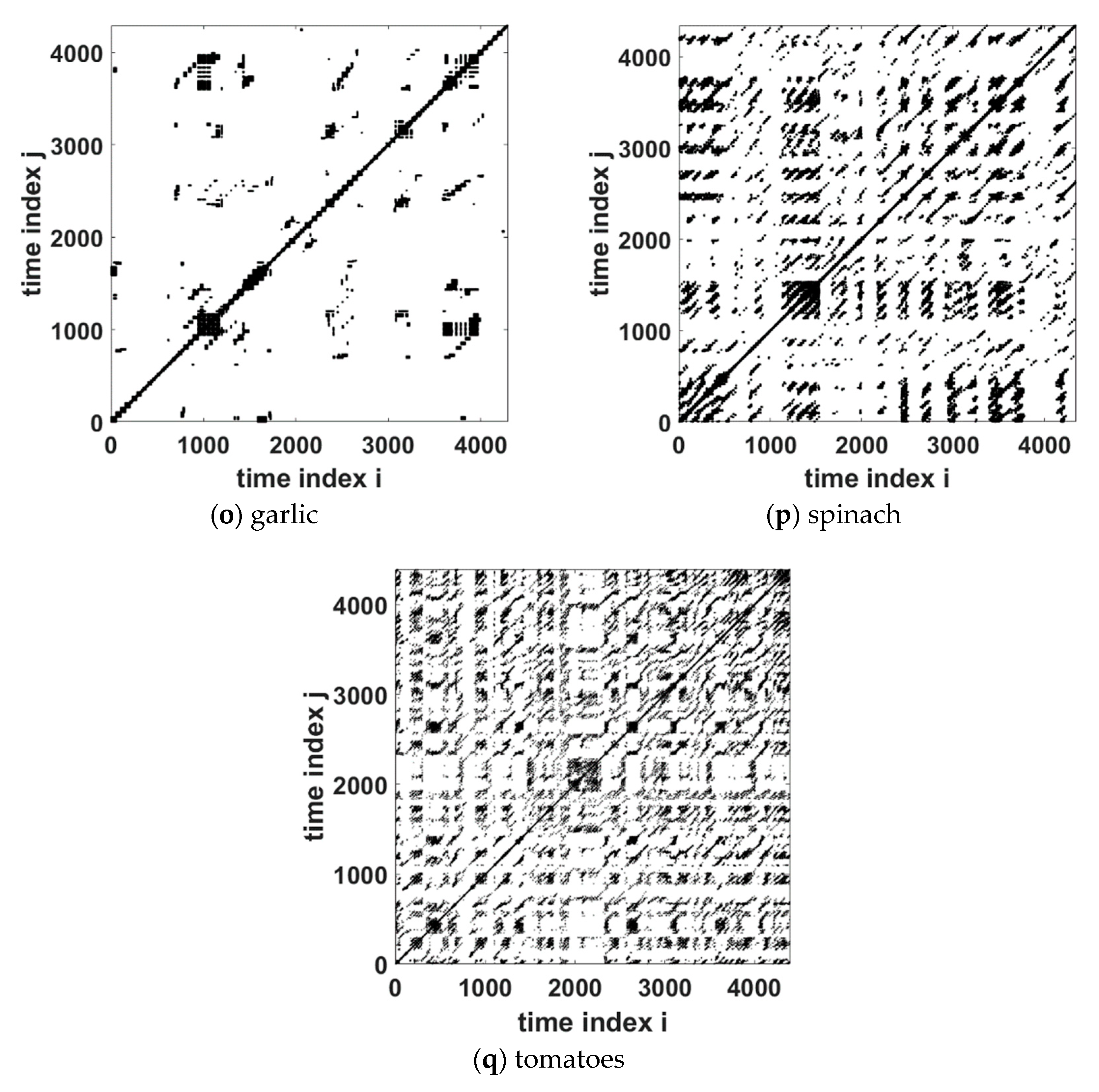
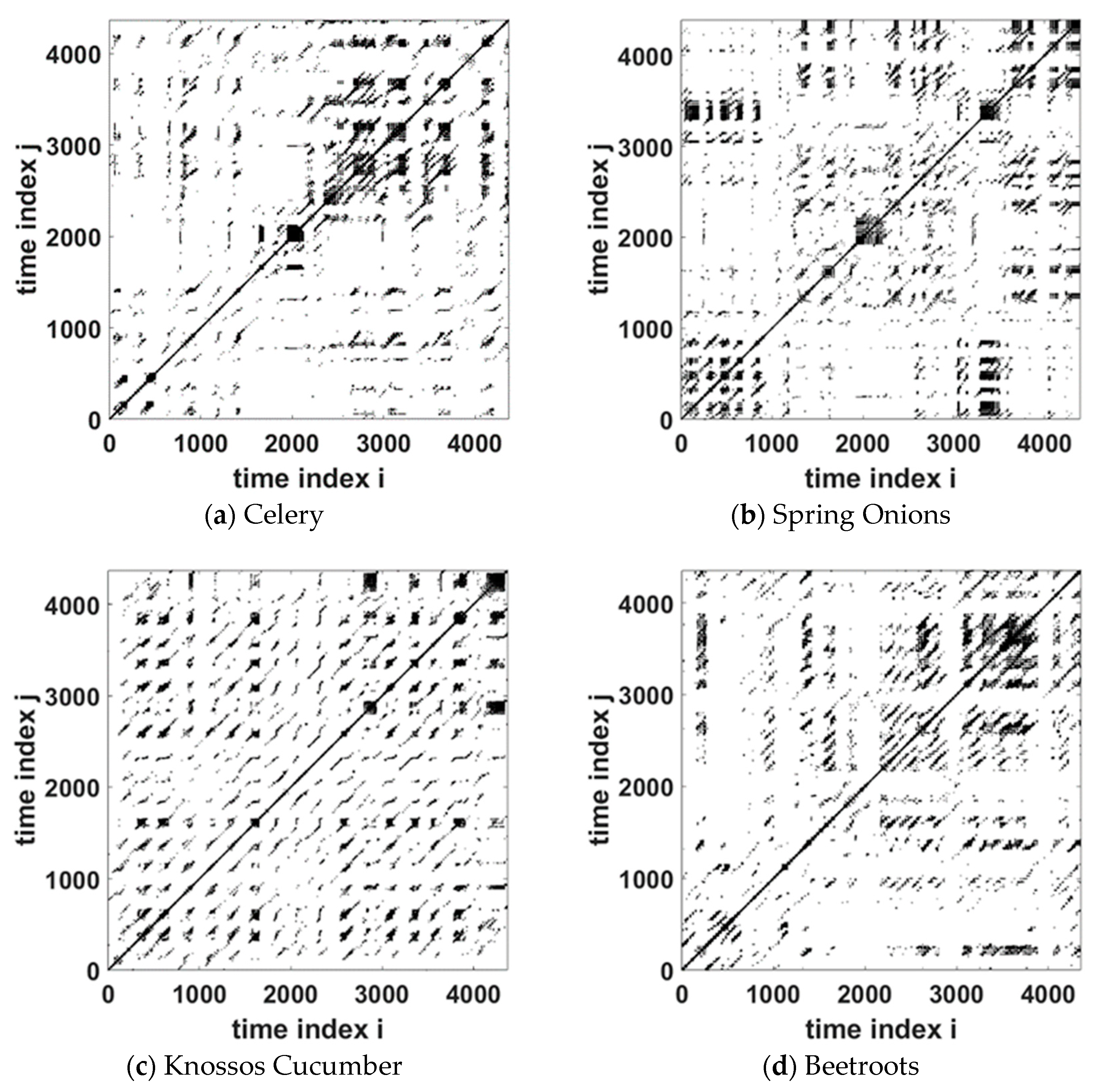
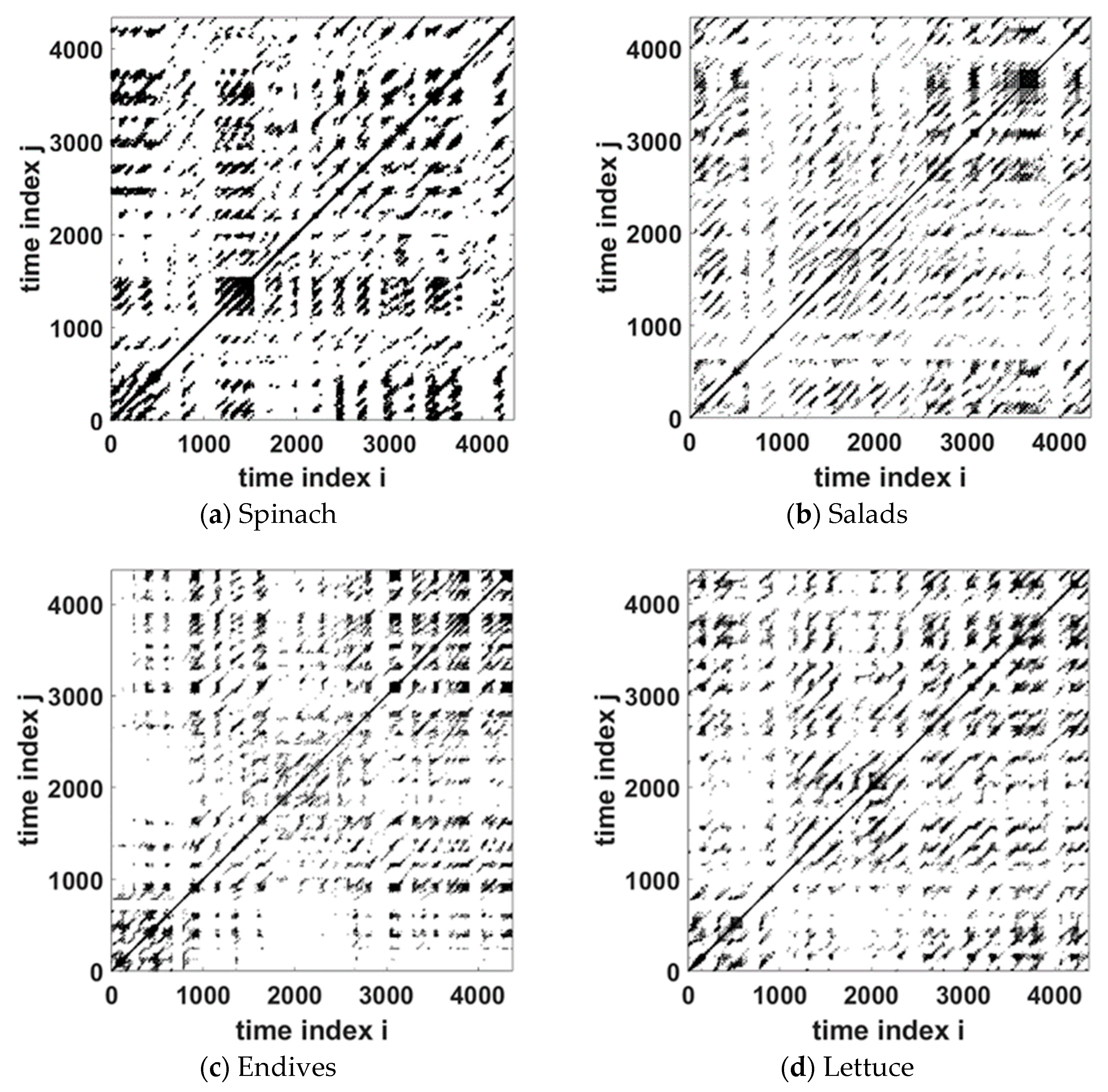
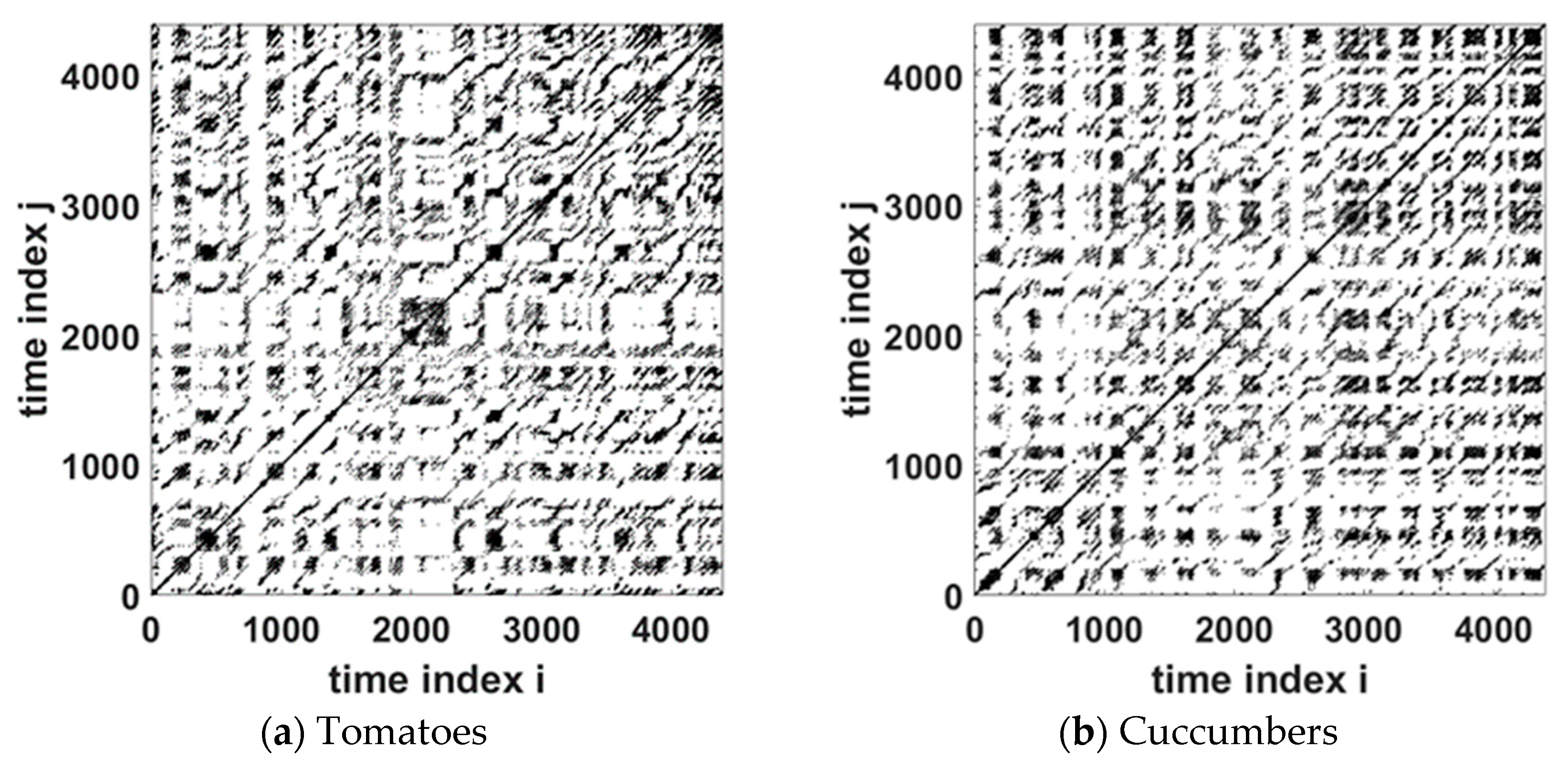
3.1. Recurrence Plots

For the calculation of Recurrence Plots, the embedding parameters of Table 2 were employed. Please note that the threshold ε was estimated with a Recurrence Rate of 0.02. As we can see, the embedding dimension for all the vegetables studied here is between 4 and 5, which also makes the comparison of RPs more direct. The resulting RPs are presented in Figure 2. We can observe that several products present relatively large delays, such as garlic, onion, and carrots. There is a range of many products that present delays in the range of 21–29 days (nearly a month) and a few products that present delays around 15 days (cucumber pair and tomatoes).
A global visual inspection of the RPs in Figure 2 leads to the following observations about patterns present in the graphs:
  • Diagonal lines parallel to the main diagonal, which vary in length and quantity depending on the case.
  • White regions, which in some cases constitute a significant part of the plot.
  • Small dark regions with a large density of diagonal and horizontal lines.
A more specific presentation of the areas of these Recurrence Plots and in which type of vegetable it is found below.
Using a visual inspection of the RPs we have performed a visual classification of the products into groups according to the visual observation of Recurrence plots and their morphology. We characterize the groups with an index vis, which stands for visual.
  • G1(vis): {Garlic, Onions, Carrots, Dill—Parsley}
We observe for this group (Figure 3) the presence of large white areas and small areas with high spot density and quite long lines. In such cases, overall price disturbances (white regions) occur over time while there are periods of time corresponding to diagonal lines formed, indicating more deterministic behavior during that time as well isolated points along lines indicating short perturbations.
  • G2(vis) {Celery, Spring onions, Knossos cucumbers, Beetroots}
In this case (Figure 4), we observe the presence of smaller parts of the RPs corresponding to white areas and small areas with a high density of spots, along with the presence of small diagonal lines. This behavior indicates states that are strongly correlated for a short time and are also disassociated for a short time. They do not last long in time, and this is also reflected in the trapping time, as we will discuss later (see Table 2), which is smaller than that of products of Group G1(vis).
The prices of vegetables in group G2(vis) for some short periods of time remain at stable levels without any particular fluctuations, unlike other periods of time, where they present larger fluctuations, as can be verified by the corresponding time-series plots in Figure 1. We can also see that we have distance between lines parallel to the diagonal ranging from around 250 (a year) and smaller, as can be seen in the corresponding time series of the products in Figure 1.
  • G3(vis) {Coarse peppers. Long-fruited peppers. Zucchini}.
The morphology of Recurrence Plots in this group (Figure 5) presents relatively large diagonal lines parallel to the main diagonal, which is evidence of determinism. The fact that we have lines parallel to the diagonal with a distance between them of about 250 points corresponding to a year (only working days), which is a sign of periodic behavior that can also be verified quite easily on the plots of the time series, with some perturbation that occur and as a result, the lines do not continue as it can be seen in Figure 5.
  • G4(vis) = {Spinach, Salads, Endives, Lettuce}
This group consists of RPs (Figure 6) with diagonal lines parallel to the main diagonal not very long, in addition to some white areas of not a large area and small dark areas are observed, which differentiates them from Figure 5 (G3(vis)) discussed previously.
There are varied dynamics in this group, with situations “trying” to be preserved in time and become deterministic. However, changes in dynamics prevail very often, and this can be seen also in the corresponding time series. The very low number of isolated points indicates the rapid recurrence of prior situations without significant disruption of pre-existing dynamics. These perturbations are the cause for the resulting small trapping times and lower determinism than the previous groups, as can be seen in Table 3.
  • G5(vis): {Tomatoes. cucumbers}
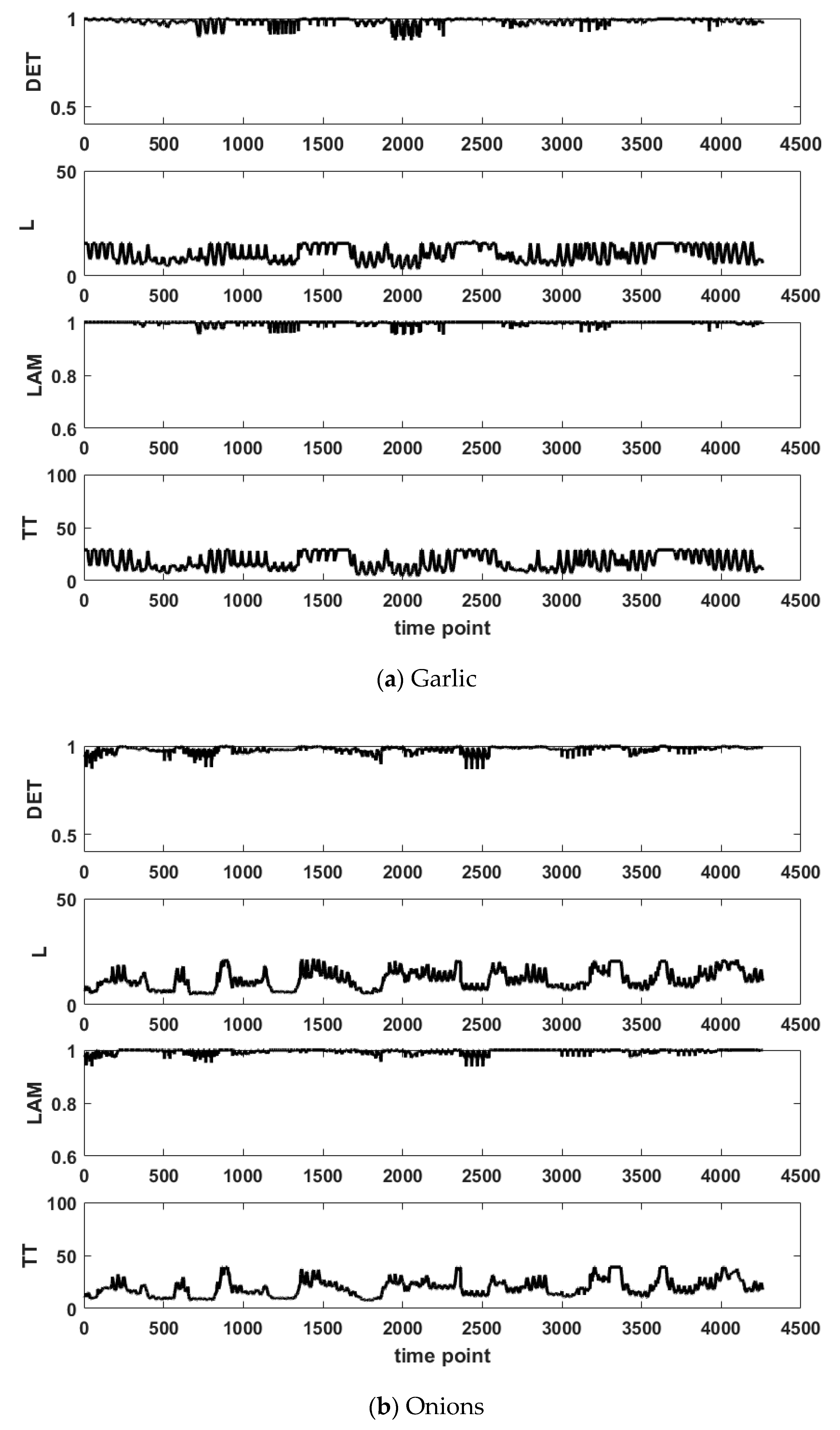
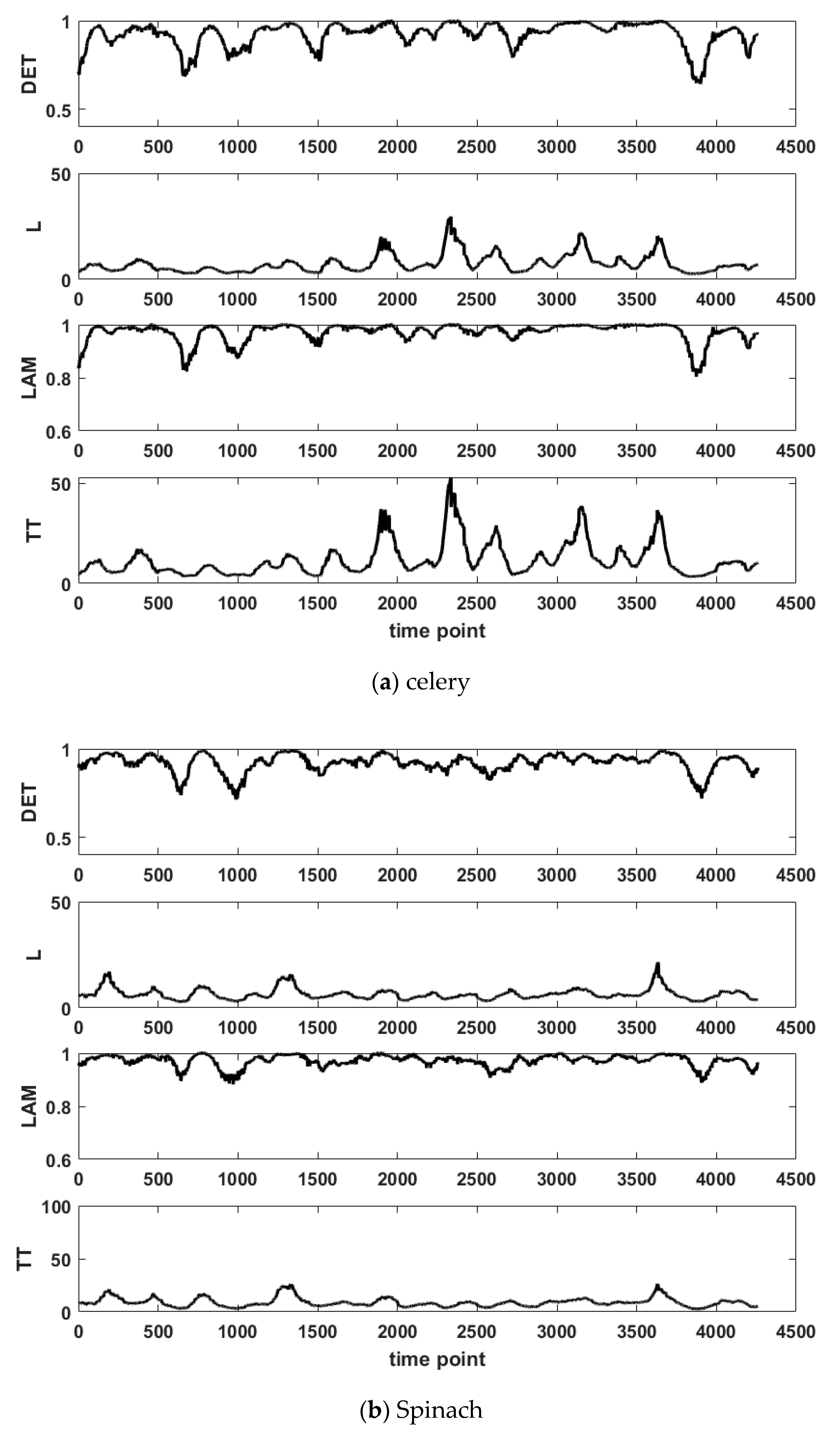
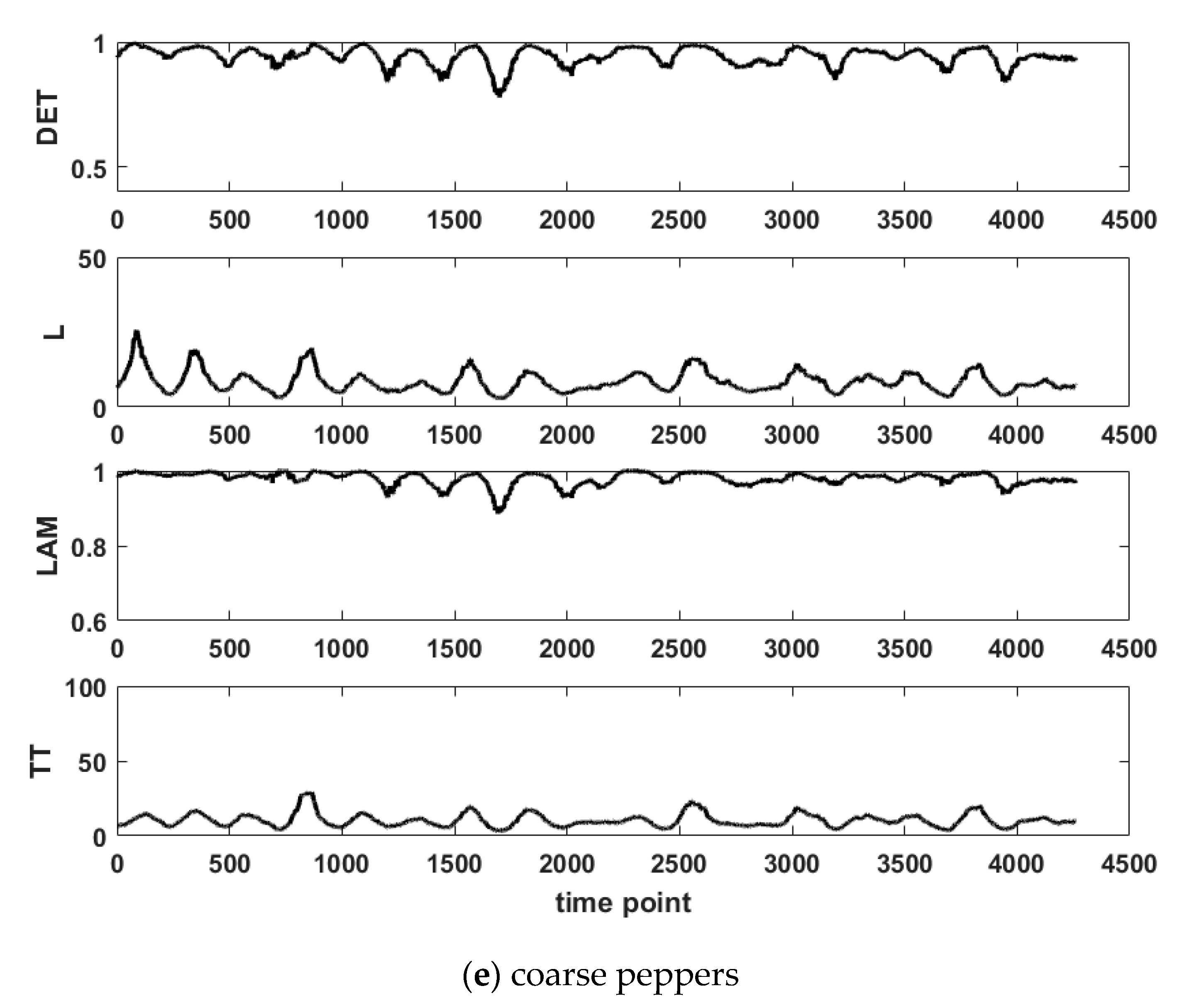
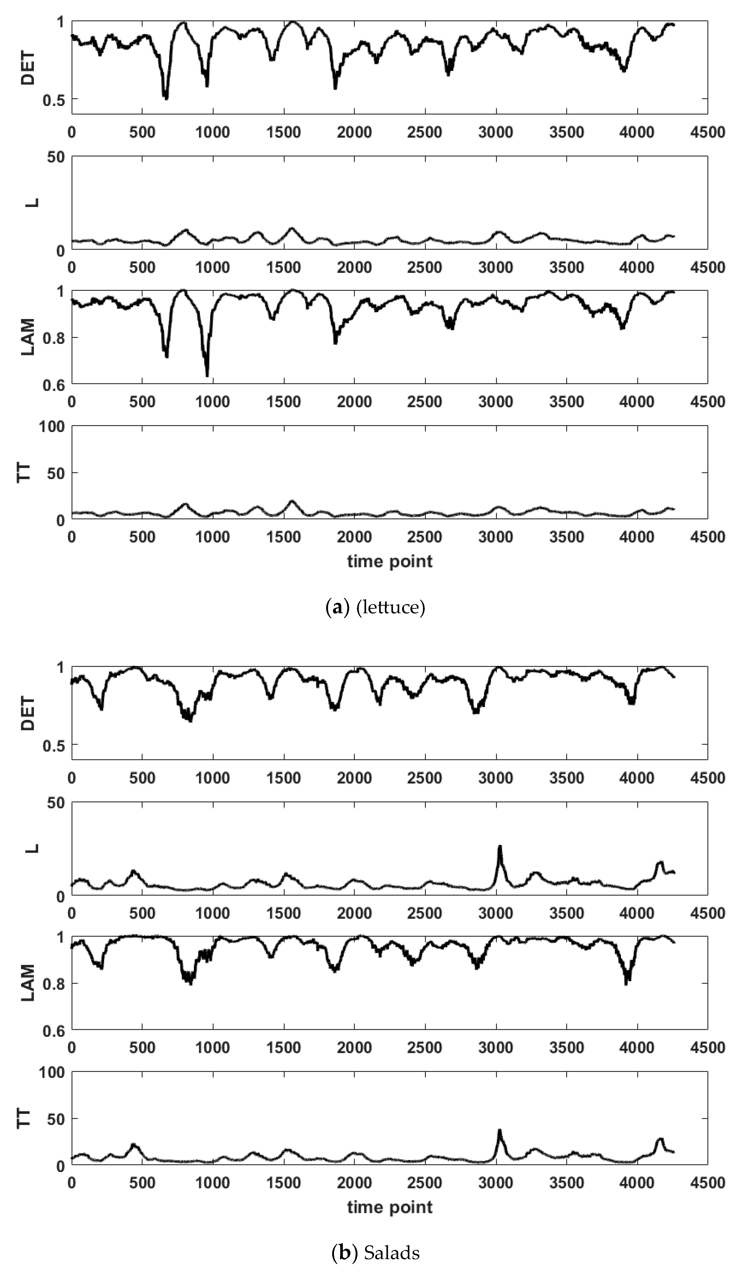
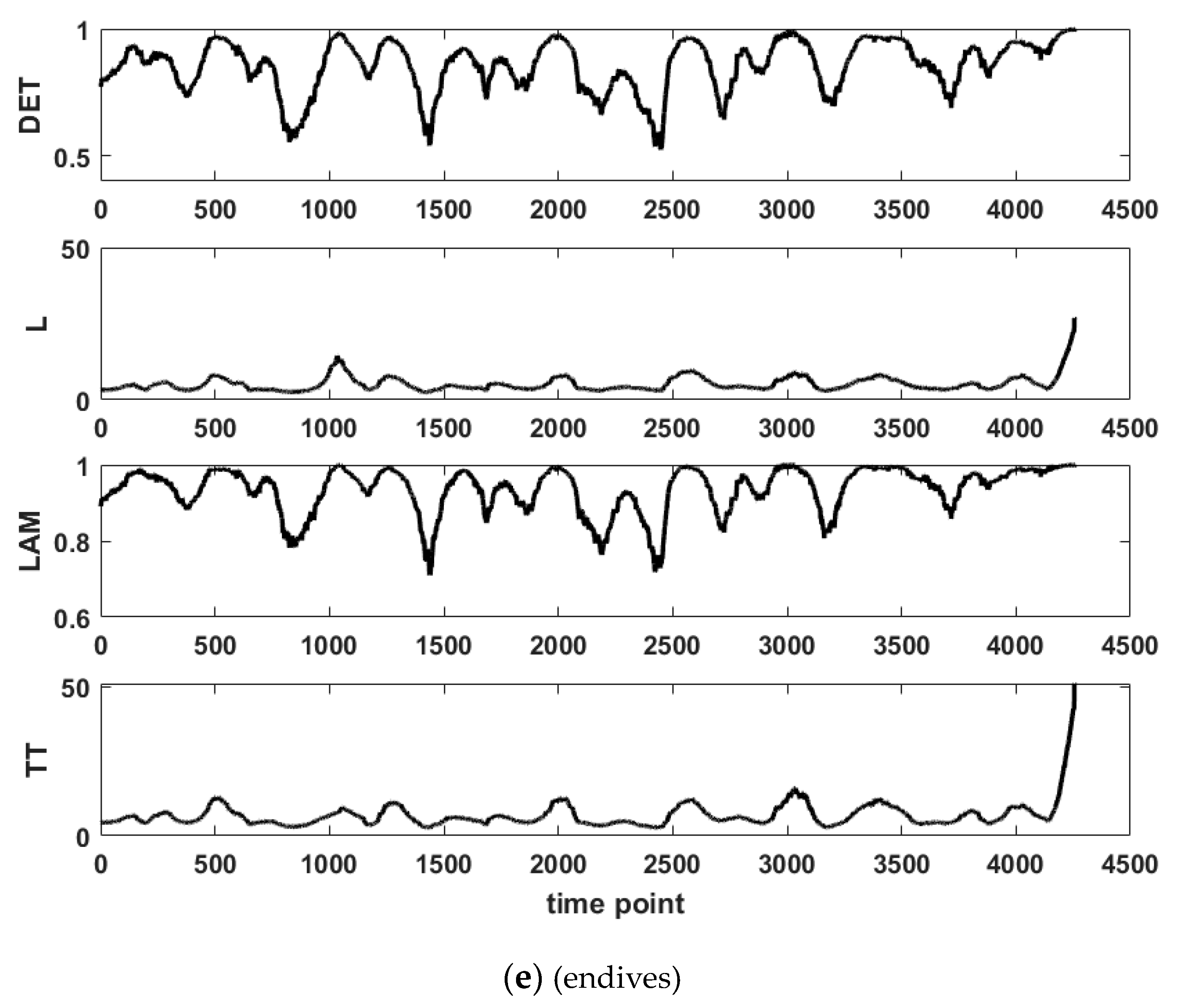
In this case, we can see in the RPs (Figure 7) that there are small regions of diagonal and vertical lines nearly all along the RPs, with small interruptions indicating frequent perturbations. This is reflected in the lowest values of determinism and trapping time that these products present (see Table 3).

3.2. RQA Results

The results of the global RQA analysis are summarized in Table 2. We can observe the important variation of TT for the products from as large as 26.723 for garlic (nearly a month) to 4.167 for cucumbers.
As we have already discussed during the presentation, based on the visual inspection of RPs the RQA quantities reflect the dynamics present on the plot. However, in order to have a more objective classification, we employed a hierarchical clustering based on all metrics of RQA analysis, and the clusterogram is presented in Figure 8a. On the vertical axis, we have the groups formed by the products, and on the horizontal axis, the groups formed by the RQA properties. It is clear that properties TT and L form one group while DET and LAM form another group. In Figure 8b, we see the groups formed (already in Figure 8a) for clarity reasons. Following the knee algorithm, a distance of 2 was chosen, resulting in the following five groups for the vegetables that we discuss below.
We can see that there are the following groups based on the clustering procedure. We use the (clust) index to refer to them.
  • G1(clust) = {Garlic-id1}
  • G2(clust) = {Onion-id2, Carrots-id3, Dill-Parsley-id4}
  • G3(clust) = {Celery-id5, Knossos cucumbers-id6, beetroots-id7, spring onions-id8, coarse peppers-id9}
  • G4(clust) = {long-fruited peppers-id10, spinach-id12, zucchini-id11, salads-id12, endives-id14}
  • G5(clust) = {tomatoes-id16, cucumbers-id17, lettuce-id15}
The groups present similarities with the ones obtained through visual inspection but also some variations. This is because clustering takes into account more details than the simple visual inspection, which, however, seems to provide a good first idea.
It is of interest to examine if the groups seem to be related to the cultivating/preservation period and the use of the products.
  • G1(clust)
Garlic is a special product used for giving taste to many dishes and is available all year round since it can be stored for a long period, thus resulting in constant availability and relative price stability, which is reflected in the largest TT among all products and the same holds for DET too.
  • G2(clust)
Onions are employed in many dishes and salads and are available all year round, too, along in some periods with the production of fresh onions leading to large DET and TT.
Carrots are employed in salad and dishes, too, and are available all year round, corresponding, too, to large DET and TT.
Dill-parsley are employed also in many dishes and salads and are available all year round.
We must remind here that the products of Groups G1(clust) and G2(clust) constituted the G1(vis) based on the visual inspection of RPs.
  • G3(clust)
Celery is a more special vegetable employed in some dishes and in salads but less than the previous products of G1(clust) and G2(clust).
Knossos cucumbers are produced in the greenhouse and are available all year round; however, in some periods, there is increased demand and, thus, price variability.
Beetroots employed in salads are used fresh, but also, in more recent times, they are employed by companies that prepare ready-to-use as well as conserved products, so there is a nearly continuous production, and the price is affected by the presence of the other forms of the same product available in the market.
Spring onions there is an increased production all year with increased use in dishes and salads during spring and summer and less during winter.
Coarse peppers are used in dishes and salads. They are very much employed in a popular dish of stuffed peppers, which is also a touristic dish, especially in the touristic period from late spring to early fall, resulting in an “average” TT compared to all products studied here.
It is of interest that celery, spring onions, Knossos cucumbers and beetroots were classified on group G2(vis) based on the visual inspection (coarse peppers were classified on group G3(vis)).
  • G4(clust)
Long-fruited peppers are mostly employed in salads and the same conserved products.
Spinach is also used as food (in dishes, pies) and salads. It is not produced all year round, but it is commonly stored in frozen form and used all around the year. This availability plays a role in the price of fresh spinach.
Zucchini is a different product employed in special dishes and as appetizers, especially in summer. We observe a difference in Period A.
Salads are like lettuce but, in general, are slightly more expensive and are used in salad plates very much.
Summarizing this group contains mainly dish-oriented products along with salad dishes. Some of the products were classified in G4(vis){spinach, salads, endives} while some in G3(vis) {zucchini, long-fruited peppers}
  • G5(clust)
We have tomatoes from greenhouses and in the field all year; however, the combined production creates perturbance to the price. While tomatoes are used in salads and dishes, many salads are extensively used during religious fasting. The same holds for cucumbers and lettuce.
Summarizing, this last group has mainly vegetables employed in salads.
It is of interest that tomatoes and cucumbers were classified from visual inspection on G5(vis).
This analysis shows that visual inspection can help mostly distinguish the difference in price behavior, but the RQA analysis provides a more detailed analysis, which, along with a clustering procedure, can help classify products. The interesting point is that the clustering reveals the dynamics related to the different uses of products and their type of cultivation, yearlong or not.

3.3. Recurrence Analysis with Epochs

However, the RQA of the whole RP presents a global behavior not presenting details in variation. In the next section, we present the epoch analysis, and we group them. The sliding window consists of a period of 180 points, i.e., one semester. Below, we present the Groups formed based on visual inspection of the time evolution of RQA quantities.
  • G1 (epochs) = {onions, garlic}
In Figure 9a, we see the results for garlic and in Figure 9b for onions. We observe that parameters present very large values, but there are some very frequent local fluctuations. We see that these products present a similar behavior. Moreover, in Table 4, we present the range of variation of the RQA parameters. We observe very high levels of determinism (most frequent DET values are from 0.986 to 1). The lowest DET value is 0.869. Some abrupt fluctuations are present along with high values of laminarity (most frequent LAM values are from 0.996 to 1), including relatively long-lasting and high-valued trapping time. It keeps the maximum value of 39 for almost 70 days. Some fluctuations are present around these values, with the most frequent trapping time values from 28 to 30. This long-lasting behavior may appear since both onions and garlic can be stored and thus can be available and consumed throughout the year compared to the other vegetables studied here, which cannot be preserved for so long periods.
  • G2(epochs) = {Carrots, Dill-Parsley)
In this case, the graphs are presented in Figure 10, and the range of values is in Table 5. We can see that we have large values with some short periods where a reduction of determinism and laminarity occurs, while in some others, an increase of trapping time to large values is observed.
For some time periods, large and sharp decreases in values are observed, reaching the value of the DET parameter at 0.408 and the value of the LAM parameter at 0.556. Possible economic events abruptly influence the dynamic behavior of the prices of these two vegetables.
Trapping Time values are in the “average” levels of 20, except for some periods when they are maximized at high values up to 98, a fact that helps to highlight a large temporal stabilization in the dynamic behavior of the prices of the vegetables under study. The most frequent trapping time values are from 7.6 to 15.2.
  • G3(epochs) = {celery, spinach, beetroots, Long-fruited peppers, Coarse-grained peppers}
In Figure 11, we present the corresponding RQA epoch graphs, and in Table 6, the range of values of RQA quantities. The values of the DET and LAM parameters show some fluctuations but do not decrease sharply. No major value drops are observed. The maximum values are kept high near 1. The minima do not fall below 0.642 for the DET parameter and 0.804 for the LAM parameter.
Trapping Time takes a value up to 53.114, not for a continuous period of time (it is a local maximum). Some “averaged” values around 25 are maintained for long periods of time. Yet, the most frequent trapping time values are from 3 to 10, which is low enough.
Again, we can see the characteristics of the various products already discussed in the case of clustering.
  • G4(epochs) = {Lettuce, Salads, Spring onions, Knossos Cucumber, Endives}
In Figure 12, we present the corresponding epoch graphs, and in Table 7, the range of RQA parameters is presented. The values of the DET and LAM parameters remain high but are slightly lower than the previous groups. In addition, continuous fluctuations occur at relatively regular intervals. Indicatively, for the DET and LAM parameters of lettuce, value variations are observed at the points from 530 to 720, 830 to 990, 1380 to 1480, 1800 to 2000, and 2600 to 2730.
In addition, large drops in the values can be seen at some points. This group contains the lowest value of DET and LAM parameters, 0.307 and 0.515, respectively. Trapping Time values varies from 2 to 62, with the most frequent values from 4.8 to 9.8.
  • G5(epochs) = {Tomatoes, Cucumber, zucchini}
In Figure 13, we have the epoch analysis graphs, and in Table 8 the range of RQA values observed. The parameters DET and LAM show values less than 1, with most of them being around 0.85. The minimum values range from 0.471 to 0.603. In general, the behavior of these parameters is oscillatory with large fluctuations. The trapping time parameter does not exceed 17.175 and is maintained at low levels, with most observations around 5, an indication of the non-sustainability of states in time.
Summarizing the grouping of products for the three different ways of grouping them in the form of a table, we obtain Table 9. It is of interest that several products constantly belong to the same group, such as tomatoes and cucumbers always being in G5, Garlic always being in G1, Carrots, and Dill-Parsley always being in either G1 or G2, and Salads Endives always being in G4 and all others in neighboring groups.
First, we can see that the visual analysis of Recurrence plots gives quite a very good separation. However, the clustering based on the RQA quantities gives a more precise and objective way for the groups formed, which are based on dynamical behavior indicators, and it seems that TT and L are the most important parameters for the separation in classes.
It seems that RQA with epoch visual classification is closer to the clustering of RQA global values but catches some slight differences; for example, in the zucchini case, which presents lower TT than the other products in the class obtained by clustering or visual inspection of RPs as well as in lettuce. We believe that this is because RQA is a quantitative and epoch analysis. Although visual, it takes into account the variability of RQA quantities, which quantify the dynamics of the system of prices through the phase space reconstruction. It would be of interest in future work to employ machine learning for the classification of the graphs as images.
Furthermore, what is of interest is that the products for the different classes are related to the use of the vegetables in the preparation of dishes, the way of cultivation during the year (in a greenhouse, in the field, or combined production), and the way they can be conserved. This can be employed as a tool for classifying products based on their use to predict the type of dynamics of a product in a given market.
The RQA quantities could be useful for prediction reasons since the trapping time provides an idea of the average remaining time around a given state. The DET parameter and the trapping time indicate the system’s time stability and deterministic behavior.

4. Conclusions

Based on the above results, the quantitative analysis of the Recurrence Plots gives a more detailed picture of the evolution of the dynamics of the system under study. The RPs can be employed as the first empirical classification tool. However, the quantitative results from RQA analysis (DET, LAM, L, TT) quantify their global behavior more objectively and can better cluster the products into groups. The trapping time, along with the maximum line, could be critical for belonging to a group.
The RQA with epochs visual analysis can provide a slightly better separation, although it is perhaps less objective at the moment since it is more visual. The main advantage of the RQA method with epochs is, on the one hand, the detection of periods during which we can understand the dynamic evolution of a phenomenon and, on the other hand, the identification of specific moments of dynamic variation, which becomes essential in detecting possible events that contributed to the change in prices at that time.
The groups of products resulting from our analysis based on the RPs seem to relate to their characteristics of use as dishes as well as to the ways of cultivation, which is the first time such a result has been obtained. Future work would be interesting to examine whether we have information for products presenting similar characteristics with given ones and whether they would fall into the same group once a clustering is performed.
Estimating trapping time can give an idea of the price stability of the products. It can be employed in policies of buying and selling products from central markets, independent buyers, and the people who cultivate the products. The dynamics of the products, i.e., price stability, could also be interesting information for government policies in various directions, for example, what products to cultivate for more excellent stability, identify for fluctuating prices, etc. It can also be an indicator for the horizon of safe prediction of prices with various models, and this could also be part of future work.
Furthermore, in the frame of future works, since it seems that RQA with epochs provides more subtle results of the dynamics, an extension of the work would be a machine-learning algorithm combining RQA measurements along with the similarity of epoch graphs, an idea similar to that of [35,36].
The above procedure for clustering products can also be extended in the future for products that are not available throughout the year by finding periods of coexistence since RPs cannot treat missing values.

Author Contributions

Conceptualization, L.Z.; Methodology, S.K. and T.K.; Software, A.F.; Formal analysis, S.K.; Data curation, S.K.; Writing—original draft, S.K.; Writing—review and editing, L.Z.; Visualization, A.F. and S.K.; Supervision, L.Z.; Project administration, L.Z. All authors have read and agreed to the published version of the manuscript.

Funding

This research received no external funding.

Informed Consent Statement

Not applicable.

Data Availability Statement

Data are available on request from the corresponding author.

Acknowledgments

The authors would like to thank the administration of the Thessaloniki Central Market for providing access to the handwritten data used in the research.

Conflicts of Interest

The authors declare no conflicts of interest.

References

  1. Claro, R.M.; Carmo, H.C.E.d.; Machado, F.M.S.; Monteiro, C.A. Income, Food Prices, and Participation of Fruit and Vegetables in the Diet. Rev. Saúde Pública 2007, 41, 557–564. [Google Scholar] [CrossRef] [PubMed]
  2. Miller, V.; Yusuf, S.; Chow, C.K.; Dehghan, M.; Corsi, D.J.; Lock, K.; Popkin, B.; Rangarajan, S.; Khatib, R.; Lear, S.A.; et al. Availability, Affordability, and Consumption of Fruits and Vegetables in 18 Countries across Income Levels: Findings from the Prospective Urban Rural Epidemiology (PURE) Study. Lancet Glob. Health 2016, 4, e695–e703. [Google Scholar] [CrossRef]
  3. French, S.A. Pricing Effects on Food Choices. J. Nutr. 2003, 133, 841S–843S. [Google Scholar] [CrossRef]
  4. Cassady, D.; Jetter, K.M.; Culp, J. Is Price a Barrier to Eating More Fruits and Vegetables for Low-Income Families? J. Am. Diet. Assoc. 2007, 107, 1909–1915. [Google Scholar] [CrossRef]
  5. Li, Y.; Liu, J.; Yang, H.; Chen, J.; Xiong, J. A Bibliometric Analysis of Literature on Vegetable Prices at Domestic and International Markets—A Knowledge Graph Approach. Agriculture 2021, 11, 951. [Google Scholar] [CrossRef]
  6. Hameed, A.A.A. The Impact of Petroleum Prices on Vegetable Oils Prices: Evidence from Cointegration Tests. In Proceedings of the 3rd International Borneo Business Conference (IBBC), Kota Kinabalu, Malaysia, 15–17 December 2008. [Google Scholar]
  7. Bozma, G.; İmamoğlu, İ.K. The Effects of Gasoline Price, Real Exchange Rate and Food Price on Vegetable and Fruit Export. Uluslar. İktisadi Ve İdari İncelemeler Derg. 2023, 182–198. [Google Scholar] [CrossRef]
  8. Pal, D.; Mitra, S.K. Interdependence between Crude Oil and World Food Prices: A Detrended Cross Correlation Analysis. Phys. Stat. Mech. Its Appl. 2018, 492, 1032–1044. [Google Scholar] [CrossRef]
  9. Moradi, M.; Salehi, M.; Keivanfar, M. A Study of the Effect of Oil Price Fluctuation on Industrial and Agricultural Products in Iran. Asian J. Qual. 2010, 11, 303–316. [Google Scholar] [CrossRef]
  10. Du, W.; Wu, Y.; Zhang, Y.; Gao, Y. The Impact Effect of Coal Price Fluctuations on China’s Agricultural Product Price. Sustainability 2022, 14, 8971. [Google Scholar] [CrossRef]
  11. Yang, H.; Cao, Y.; Shi, Y.; Wu, Y.; Guo, W.; Fu, H.; Li, Y. The Dynamic Impacts of Weather Changes on Vegetable Price Fluctuations in Shandong Province, China: An Analysis Based on VAR and TVP-VAR Models. Agronomy 2022, 12, 2680. [Google Scholar] [CrossRef]
  12. Qiao, Y.; Kang, M.; Ahn, B. Analysis of Factors Affecting Vegetable Price Fluctuation: A Case Study of South Korea. Agriculture 2023, 13, 577. [Google Scholar] [CrossRef]
  13. Beniwal, A.; Poolsingh, D.; Shastry, S.S. Trends and Price Behaviour Analysis of Onion in India. Indian J. Agric. Econ. 2022, 77, 632–642. [Google Scholar] [CrossRef]
  14. Birthal, P.; Negi, A.; Joshi, P.K. Understanding Causes of Volatility in Onion Prices in India. J. Agribus. Dev. Emerg. Econ. 2019, 9, 255–275. [Google Scholar] [CrossRef]
  15. Shengwei, W.; Yanni, L.; Jiayu, Z.; Jiajia, L. Agricultural Price Fluctuation Model Based on SVR. In Proceedings of the 2017 9th International Conference on Modelling, Identification and Control (ICMIC), Kunming, China, 10–12 July 2017; pp. 545–550. [Google Scholar]
  16. Jin, D.; Yin, H.; Gu, Y.; Yoo, S.J. Forecasting of Vegetable Prices Using STL-LSTM Method. In Proceedings of the 2019 6th International Conference on Systems and Informatics (ICSAI), Shanghai, China, 2–4 November 2019; pp. 866–871. [Google Scholar]
  17. Charakopoulos, A.; Karakasidis, T.; Sarris, L. Pattern Identification for Wind Power Forecasting via Complex Network and Recurrence Plot Time Series Analysis. Energy Policy 2019, 133, 110934. [Google Scholar] [CrossRef]
  18. Sankararaman, S. Recurrence Network and Recurrence Plot: A Novel Data Analytic Approach to Molecular Dynamics in Thermal Lensing. J. Mol. Liq. 2022, 366, 120353. [Google Scholar] [CrossRef]
  19. Pitsik, E.; Frolov, N.; Hauke Kraemer, K.; Grubov, V.; Maksimenko, V.; Kurths, J.; Hramov, A. Motor Execution Reduces EEG Signals Complexity: Recurrence Quantification Analysis Study. Chaos Interdiscip. J. Nonlinear Sci. 2020, 30, 023111. [Google Scholar] [CrossRef] [PubMed]
  20. Andreadis, I.; Fragkou, A.D.; Karakasidis, T.E.; Serletis, A. Nonlinear Dynamics in Divisia Monetary Aggregates: An Application of Recurrence Quantification Analysis. Financ. Innov. 2023, 9, 16. [Google Scholar] [CrossRef]
  21. Fragkou, A.D.; Karakasidis, T.E.; Sarris, I.E. Recurrence Quantification Analysis of MHD Turbulent Channel Flow. Phys. Stat. Mech. Its Appl. 2019, 531, 121741. [Google Scholar] [CrossRef]
  22. Charakopoulos, A.Κ.; Karakasidis, T.E.; Papanicolaou, P.N.; Liakopoulos, A. The Application of Complex Network Time Series Analysis in Turbulent Heated Jets. Chaos Interdiscip. J. Nonlinear Sci. 2014, 24, 024408. [Google Scholar] [CrossRef]
  23. Eckmann, J.-P.; Kamphorst, S.O.; Ruelle, D. Recurrence Plots of Dynamical Systems. Europhys. Lett. 1987, 4, 973. [Google Scholar] [CrossRef]
  24. Takens, F. Detecting Strange Attractors in Turbulence. In Dynamical Systems and Turbulence, Warwick 1980: Proceedings of the Symposium Held at the University of Warwick 1979/80; Rand, D., Young, L.-S., Eds.; Springer: Berlin/Heidelberg, Germany, 1981; pp. 366–381. [Google Scholar]
  25. Packard, N.H.; Crutchfield, J.P.; Farmer, J.D.; Shaw, R.S. Geometry from a Time Series. Phys. Rev. Lett. 1980, 45, 712–716. [Google Scholar] [CrossRef]
  26. Fraser, A.M.; Swinney, H.L. Independent Coordinates for Strange Attractors from Mutual Information. Phys. Rev. A 1986, 33, 1134–1140. [Google Scholar] [CrossRef] [PubMed]
  27. Abarbanel, H.D.I.; Kennel, M.B. Local False Nearest Neighbors and Dynamical Dimensions from Observed Chaotic Data. Phys. Rev. E 1993, 47, 3057–3068. [Google Scholar] [CrossRef]
  28. Zbilut, J.P.; Webber, C.L. Embeddings and Delays as Derived from Quantification of Recurrence Plots. Phys. Lett. A 1992, 171, 199–203. [Google Scholar] [CrossRef]
  29. Marwan, N.; Carmen Romano, M.; Thiel, M.; Kurths, J. Recurrence Plots for the Analysis of Complex Systems. Phys. Rep. 2007, 438, 237–329. [Google Scholar] [CrossRef]
  30. Marwan, N. TOCSY Toolbox. Available online: https://tocsy.pik-potsdam.de/ (accessed on 13 August 2024).
  31. Hegger, R.; Kantz, H.; Schreiber, T. Practical Implementation of Nonlinear Time Series Methods: The TISEAN Package. Chaos Interdiscip. J. Nonlinear Sci. 1999, 9, 413–435. [Google Scholar] [CrossRef]
  32. TISEAN: Nonlinear Time Series Analysis. Available online: https://www.pks.mpg.de/tisean/ (accessed on 13 August 2024).
  33. Sarantopoulos, A.; Korovesis, S. Effects of Climate Change in Agricultural Areas of Greece, Vulnerability Assessment, Economic-Technical Analysis, and Adaptation Strategies. Environ. Sci. Proc. 2023, 26, 173. [Google Scholar] [CrossRef]
  34. Georgopoulou, E.; Mirasgedis, S.; Sarafidis, Y.; Vitaliotou, M.; Lalas, D.P.; Theloudis, I.; Giannoulaki, K.-D.; Dimopoulos, D.; Zavras, V. Climate Change Impacts and Adaptation Options for the Greek Agriculture in 2021–2050: A Monetary Assessment. Clim. Risk Manag. 2017, 16, 164–182. [Google Scholar] [CrossRef]
  35. Barros, L.R.; Soares, G.G.P.; Correia, S.; Duarte, G.; Costa, S.C. Classification of Recurrence Plots of Voice Signals Using Convolutional Neural Networks. In Proceedings of the XXXVIII Simpósio Brasileiro de Telecomunicações e Processamento de SINAIS—SBrT 2020, Florianópolis, Brazil, 22–25 November 2020. [Google Scholar]
  36. Lansford, J.L.; Vlachos, D.G. Infrared Spectroscopy Data- and Physics-Driven Machine Learning for Characterizing Surface Microstructure of Complex Materials. Nat. Commun. 2020, 11, 1513. [Google Scholar] [CrossRef]
Figure 1. Time series for the vegetables studied in the present paper.
Appliedmath 04 00055 g001aAppliedmath 04 00055 g001bAppliedmath 04 00055 g001c
Figure 2. Recurrence Plots of vegetables studied in the paper.
Appliedmath 04 00055 g002aAppliedmath 04 00055 g002bAppliedmath 04 00055 g002cAppliedmath 04 00055 g002d
Figure 3. G1(vis) Recurrence Plots.
Appliedmath 04 00055 g003
Figure 4. G2(vis) Recurrence Plots.
Appliedmath 04 00055 g004
Figure 5. Group G3(vis) Recurrence Plots.
Appliedmath 04 00055 g005
Figure 6. Group D(vis) Recurrence Plots.
Appliedmath 04 00055 g006
Figure 7. Group Ε(vis) Recurrence Plots.
Appliedmath 04 00055 g007
Figure 8. (a) Clusterogram of the RQA quantities appearing in Table 2. (b) the clustering of the products in closer detail.
Appliedmath 04 00055 g008
Figure 9. Recurrence Quantification Analysis of G1(epochs).
Appliedmath 04 00055 g009
Figure 10. Recurrence Quantification Analysis of G2 (epochs).
Appliedmath 04 00055 g010aAppliedmath 04 00055 g010b
Figure 11. Recurrence Quantification Analysis with epochs for G3(epochs).
Appliedmath 04 00055 g011aAppliedmath 04 00055 g011bAppliedmath 04 00055 g011c
Figure 12. Recurrence Quantification Analysis with epochs for the G4(epochs) group.
Appliedmath 04 00055 g012aAppliedmath 04 00055 g012bAppliedmath 04 00055 g012c
Figure 13. Recurrence Quantification Analysis with epochs for G5(epochs).
Appliedmath 04 00055 g013aAppliedmath 04 00055 g013b
Table 1. Vegetables for which time-series analysis was performed.
Description
Cucumbers
Knossos Cucumbers
Dill, Parsley bales
Endives
Carrots
Zucchini
Spring onions, fresh bale
Onions
Lettuce
Beetroot
Long-fruited peppers
Coarse peppers
Salads
Celery
Garlic
Spinach
Tomatoes
Table 2. The embedding parameters of Recurrence Plots for each product.
ProductDelayEmbeddingThreshold
Cucumber1540.147
Knossos cucumbers2340.176
Dill—Parsley2740.0435
Endives2240.105
Carrots3540.046
Zucchini2140.25
Spring onions2530.029
Onions3550.075
Lettuce2540.185
Beetroot2940.105
Long-fruited peppers2540.33
Coarse peppers2740.41
Salads2650.34
Celery2540.18
Garlic5040.2235
Spinach2550.28
Tomatoes1640.2291
Table 3. RQA results for the RPs; all time series.
IDVegetableDETLAMLTT
1Garlic0.9910.99714.88626.723
2Onions0.9650.9879.23415.267
3Carrots0.9590.9848.86715.315
4Dill-Parsley0.9580.9838.10413.960
5Celery0.9320.9756.31810.295
6Knossos Cucumbers0.9320.9755.9779.322
7Beetroots0.9280.9755.6129.003
8Spring onions0.8970.9575.6249.203
9Coarse Peppers0.9150.9626.0368.494
10Long-fruited peppers0.8930.9545.0157.118
11Zucchini0.8360.9204.3516.057
12Spinach0.8840.9504.7967.059
13Salads0.8570.9334.4716.286
14Endives0.8510.9394.3056.466
15Lettuce0.8000.9063.8385.405
16Tomatoes0.7160.8503.2094.194
17Cucumbers0.7130.8583.1304.167
Table 4. Values per RQA quantity for G1(epochs) members. For each measure, the range of values is presented.
RQA MeasuresOnionsGarlic
DET0.869–10.876–1
L4.701–21.7273.365–17.050
LAM0.937–10.952–1
TT7.180–394.507–29
Table 5. Values for RQA measures for G2(epochs) members. For each measure, the range of values is presented.
RQA MeasuresDill-ParsleyCarrots
DET0.408–0.9990.418–0.999
L2.080–502.214–38
LAM0.556–10.627–1
TT2.229–982.485–74
Table 6. Minimum and maximum values per RQA quantity for G3(epochs).
RQA Measures CelerySpinachBeetroots Long-Fruited PeppersCoarse Peppers
DET0.642–0.9980.714–0.9920.669–0.9970.784–0.9960.777–0.998
L2.666–29.5762.775–21.4802.685–21.8783.796–26.0832.940–25.652
LAM0.804–10.882–10.815–10.918–10.885–1
TT3.341–53.1142.870–26.4402.794–37.1544.606–29.5433.510–29.085
Table 7. Values per RQA quantity for G4(epochs) members. For each measure, the range of values is presented.
RQA MeasureLettuceSaladsSpring OnionsKnossos
Cucumber
Endives
DET0.491–0.9920.640–0.9950.307–0.9970.735–0.9990.523–0.998
L2.214–11.5852.666–26.8752.181–24.3332.95–34.9232.371–26.895
LAM0.629–10.788–10.515–10.862–10.710–1
TT2.342–19.8702.745–38.4592.264–403.551–62.7452.718–51
Table 8. Values per RQA quantity for G5(epochs) members. For each measure, the range of values is presented.
RQA MeasureTomatoesCucumber PairZucchini
DET0.567–0.9620.603–0.958 0.471–0.986
L2.626–8.6272.566–6.5232.757–12.363
LAM0.716–0.9840.794–0.9860.673–0.999
TT2.735–10.6682.759–8.0412.870–17.175
Table 9. Vegetables, RQA quantities the various belonging to clusters (vis: from RPs inspection, clust, from RQA quantities clustering, epoch: from RQA epoch visual inspection.)
VegetablesDETLAMLTTG1
(Vis)
G2
(Vis)
G3
(Vis)
G4
(Vis)
G5
(Vis)
G1
(Clust)
G2
(Clust)
G3
(Clust)
G4
(Clust)
G5
(Clust)
G1
(Epoch)
G2
(Epoch)
G3
(Epoch)
G4
(Epoch)
G5
(Epoch)
Garlic0.9910.99714.88626.723
Onions0.9650.9879.23415.267
Carrots0.9590.9848.86715.315
Dill-Parsley0.9580.9838.10413.960
Celery0.9320.9756.31810.295
Knossos Cucumbers0.9320.9755.9779.322
Beetroots0.9280.9755.6129.003
Spring Onions0.8970.9575.6249.203
Coarse Peppers0.9150.9626.0368.494
Long-fruited Peppers0.8930.9545.0157.118
Zucchini0.8360.9204.3516.057
Spinach0.8840.9504.7967.059
Salads0.8570.9334.4716.286
Endives0.8510.9394.3056.466
Lettuce0.8000.9063.8385.405
Tomatoes0.7160.8503.2094.194
Cucumbers0.7130.8583.1304.167
Disclaimer/Publisher’s Note: The statements, opinions and data contained in all publications are solely those of the individual author(s) and contributor(s) and not of MDPI and/or the editor(s). MDPI and/or the editor(s) disclaim responsibility for any injury to people or property resulting from any ideas, methods, instructions or products referred to in the content.

