Abstract
Cancer, a complex disease characterized by uncontrolled cell growth and metastasis, remains a formidable challenge to global health. Mathematical modeling has emerged as a critical tool to elucidate the underlying biological mechanisms driving tumor initiation, progression, and treatment responses. By integrating principles from biology, physics, and mathematics, mathematical oncology provides a quantitative framework for understanding tumor growth dynamics, microenvironmental interactions, and the evolution of cancer cells. This study explores the key applications of mathematical modeling in oncology, encompassing tumor growth kinetics, intra-tumor heterogeneity, personalized medicine, clinical trial optimization, and cancer immunology. Through the development and application of computational models, researchers aim to gain deeper insights into cancer biology, identify novel therapeutic targets, and optimize treatment strategies. Ultimately, mathematical oncology holds the promise of transforming cancer care by enabling more precise, personalized, and effective therapies.
1. Introduction
Cancer, a multifaceted disease characterized by uncontrolled cell proliferation and metastasis, poses a significant challenge to global health. Its heterogeneity, encompassing a vast array of types and stages, necessitates innovative approaches to understand and combat its complexities. Traditional biological and clinical research, while invaluable, often falls short in capturing the intricate dynamics and interactions within the tumor microenvironment. This is where mathematical modeling emerges as a powerful and complementary tool. By translating biological processes into quantitative frameworks, mathematical oncology offers a unique perspective on tumor behavior, enabling researchers to simulate, predict, and analyze cancer progression with unprecedented precision [1,2,3]. This interdisciplinary field, merging insights from biology, physics, and mathematics, provides a comprehensive approach to unraveling the intricate mechanisms underlying cancer development, growth, and metastasis [4,5,6]. Through the construction and analysis of mathematical models, researchers can explore the complex interplay among cancer cells, immune cells, and the surrounding microenvironment, shedding light on the factors that drive tumor initiation, growth, invasion, and treatment resistance. By quantifying these interactions, mathematical oncology offers a foundation for developing targeted and effective therapeutic strategies.
Central to mathematical oncology is the modeling of tumor growth patterns and their response to therapeutic interventions. Population dynamic models, such as the logistic growth model and its extensions, have been instrumental in capturing the growth kinetics of tumors and their interactions with the surrounding microenvironment [1,2,7]. These models incorporate parameters that account for factors like cell proliferation, death, and resource availability, enabling researchers to simulate tumor growth under various conditions. Spatial heterogeneity, a hallmark of tumor progression, is another critical aspect addressed by mathematical models. Incorporating spatial factors, such as diffusion and reaction kinetics, allows for a more realistic representation of tumor growth and its interaction with the microenvironment [3,7]. This spatial perspective is essential for understanding processes like angiogenesis, invasion, and metastasis, where the physical distribution of cells and extracellular matrix components plays a crucial role. The tumor microenvironment, a complex ecosystem comprising cancer cells, immune cells, stromal cells, and extracellular matrix, significantly influences tumor behavior. Mathematical models have been employed to investigate how interactions within this microenvironment contribute to tumor growth, invasion, and treatment resistance [3]. By capturing the dynamic interplay between these cellular and molecular components, these models offer insights into the mechanisms underlying tumor progression and treatment responses. Furthermore, mathematical models have been used to explore the impact of physical forces, such as fluid shear stress and mechanical strain, on tumor growth and metastasis. These studies have highlighted the importance of integrating biophysical factors into cancer modeling to gain a more comprehensive understanding of tumor behavior.
Cancer is not a monolithic entity but a complex ecosystem characterized by remarkable heterogeneity. Tumor cells exhibit diverse genetic, phenotypic, and metabolic characteristics, contributing to the challenges of diagnosis, treatment, and prognosis [8,9]. Mathematical models have proven invaluable in unraveling the intricacies of this heterogeneity and its implications for cancer progression. By incorporating evolutionary principles, mathematical models can simulate the process of clonal expansion, diversification, and selection within tumors. These models help to elucidate how genetic and phenotypic variations arise, leading to the emergence of drug-resistant subclones and the potential for metastasis [8]. Understanding the mechanisms driving intra-tumor heterogeneity is crucial for developing effective therapeutic strategies that can target and eliminate diverse tumor cell populations. Furthermore, mathematical models can be employed to investigate the role of cellular plasticity in cancer progression. The ability of cancer cells to undergo phenotypic changes in response to environmental cues, such as therapeutic pressure, contributes to tumor heterogeneity and treatment resistance. By modeling these dynamic processes, researchers can gain insights into the mechanisms underlying cellular plasticity and develop strategies to target this adaptive capacity.
The advent of personalized medicine has ushered in an era of tailored cancer treatment, emphasizing the importance of individual patient characteristics in guiding therapeutic decisions. Mathematical models have emerged as indispensable tools for realizing the potential of this paradigm shift [10,11]. The immune system serves as a crucial line of defense against cancer, with immune cells capable of recognizing and eliminating tumor cells. However, cancer cells often develop strategies to evade immune surveillance, leading to immune escape and treatment resistance. Mathematical models have been instrumental in unraveling the complex interplay between cancer cells and immune cells, providing valuable insights into the mechanisms underlying these processes [12,13]. By quantifying the interactions between different immune cell types, such as T cells, B cells, natural killer cells, and myeloid-derived suppressor cells, with cancer cells, mathematical models can elucidate the dynamics of the immune response to tumors. These models can capture the complex feedback loops and signaling pathways that regulate immune activation, proliferation, and effector functions, as well as tumor-induced immune suppression [12]. Furthermore, mathematical models have been employed to investigate the mechanisms of immune escape, including the development of immune checkpoints, antigen loss, and the creation of immunosuppressive tumor microenvironments. By understanding these escape mechanisms, researchers can develop strategies to overcome immune evasion and enhance the efficacy of immunotherapy [13]. In addition to informing our understanding of the immune response to cancer, mathematical models have been used to optimize immunotherapy strategies. By simulating the effects of different immunotherapy approaches, such as checkpoint inhibitors, adoptive cell therapy, and cancer vaccines, researchers can identify optimal treatment combinations and predict patient outcomes [14,15].
By integrating patient-specific data, such as genomic profiles, imaging biomarkers, and clinical history, into computational models, researchers can simulate tumor growth and the response to various treatment options, enabling the selection of optimal therapeutic strategies for individual patients. This precision medicine approach holds the promise of maximizing treatment efficacy while minimizing adverse effects [16,17]. Moreover, mathematical modeling plays a pivotal role in optimizing clinical trial design and execution. By simulating the effects of different treatment regimens under varying patient populations, researchers can identify optimal trial endpoints, patient selection criteria, and sample sizes [14,15]. This data-driven approach accelerates the drug development process, reduces costs, and increases the probability of successful clinical trials. Ultimately, the integration of mathematical modeling into clinical practice has the potential to revolutionize cancer care by enabling more effective and personalized treatment strategies.
This study elaborates on the key applications of mathematical modeling in oncology, encompassing tumor growth kinetics, microenvironmental interactions, evolutionary dynamics, personalized medicine, clinical trial optimization, and cancer immunology. Through the integration of experimental data and computational modeling, mathematical oncology holds the potential to revolutionize cancer research and improve patient outcomes.
2. Mathematical Modeling of the Tumor Microenvironment
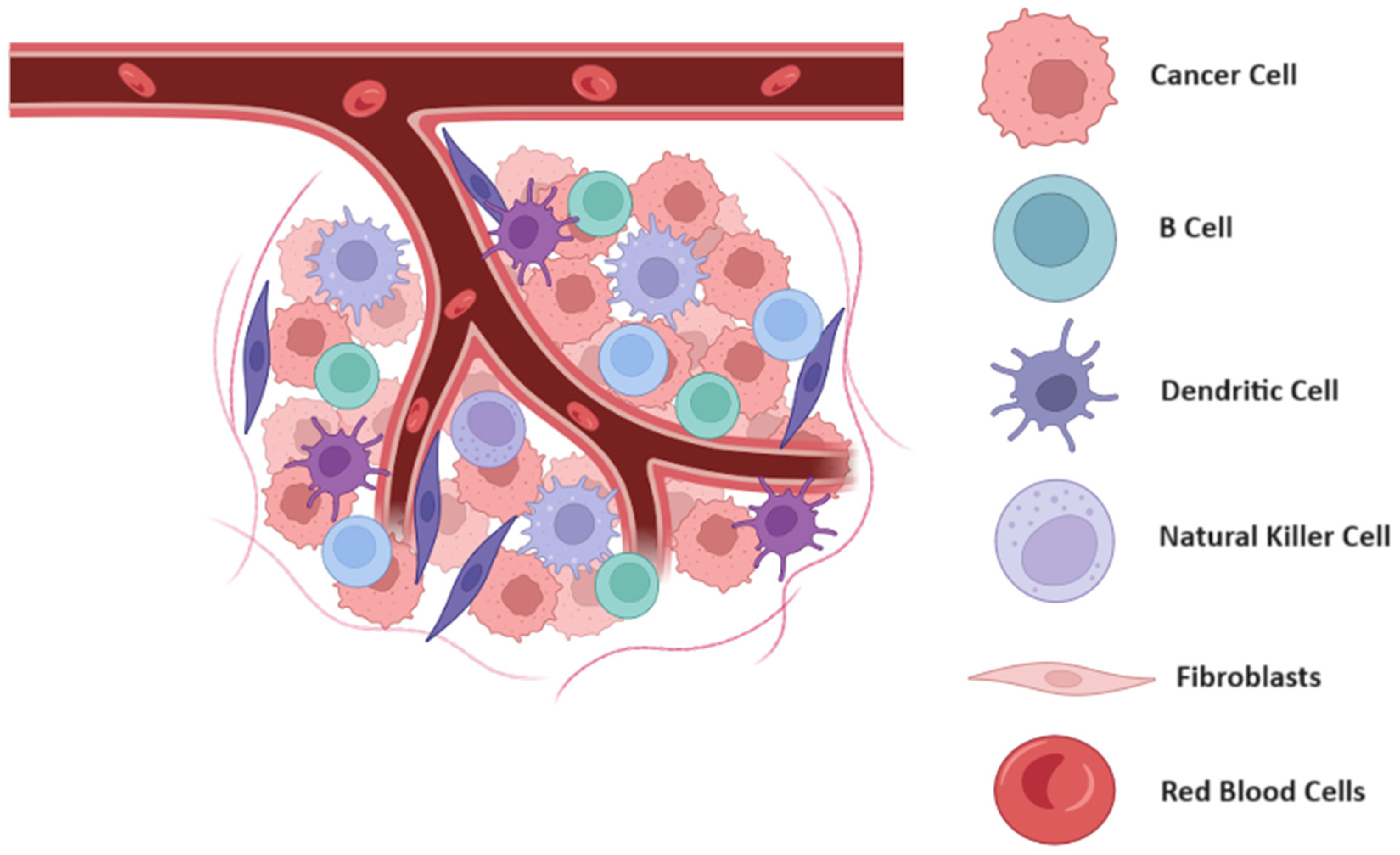
Recent advancements in mathematical modeling have significantly enhanced our understanding of the tumor microenvironment (TME) (see Figure 1), emphasizing its complexity and heterogeneity. These models integrate various biological, physical, and chemical processes to simulate the interactions between cancer cells and their surrounding stromal and immune components. For instance, sophisticated models have been developed to capture the dynamics of tumor angiogenesis, the immune response, and the influence of the extracellular matrix on cancer progression [18,19,20,21,22]. Such models are crucial for predicting tumor behavior under different therapeutic scenarios, enabling personalized treatment strategies and optimizing clinical outcomes. By providing a detailed representation of the TME, mathematical models are pivotal in identifying potential therapeutic targets and understanding the mechanisms of resistance, thereby paving the way for more effective cancer treatments.

Figure 1.
Schematic representation of tumor microenvironment and its dynamic interactions. This schematic illustrates the complex interactions within the tumor microenvironment (TME), highlighting the key components and their roles in tumor progression. The TME comprises cancer cells, stromal cells, immune cells, and extracellular matrix, all interacting through various signaling pathways. These interactions influence tumor growth, metastasis, and the response to therapy. The diagram emphasizes the spatial and functional heterogeneity of the TME, showcasing how different cellular and molecular components contribute to the adaptive and often resistant nature of tumors. Figure created using Biorender.
Reaction–diffusion–advection (RDA) models are mathematical models used to simulate the spatiotemporal dynamics of biochemical substances, such as nutrients, growth factors, and signaling molecules, within the tumor microenvironment (see Algorithm 1). These models incorporate processes of diffusion, advection, and chemical reactions to study how molecular species propagate and interact within the tissue.
| Algorithm 1. Reaction–Diffusion Simulation |
| Initialize chemo_grid with initial_chemo_concentration |
| Initialize immune_grid with zeros |
| For each iteration in 1 to num_iterations: |
| Create chemo_next as a copy of chemo_grid |
| For each cell (i, j) in the grid excluding boundaries: |
| Compute laplacian using neighboring cells |
| Update chemo_next(i, j) using diffusion, decay, and production rates |
| Update chemo_grid with chemo_next |
| For each cell (i, j) in the grid: |
| Compute recruitment_prob based on chemo_grid(i, j) |
| If random() < recruitment_prob: |
| diffusion_coefficient = 0.1; % Diffusion coefficient for chemoattractant |
| tumor_production_rate = 0.5; % Rate of chemoattractant production by tumor cells |
| immune_production_rate = 0.2; % Rate of immune cell production |
| decay_rate = 0.1; % Rate of decay for chemoattractant |
The general form of the reaction–diffusion–advection equation can be expressed as follows:
where C represents the concentration of a molecular species (e.g., oxygen, nutrients, growth factors) as a function of spatial coordinates (x, y, z) and time (t). D is the diffusion coefficient, representing the rate at which the molecule diffuses through the tissue. v is the advection velocity vector, indicating the bulk flow or convective transport of the molecule due to fluid flow within the tissue. R(C) represents the reaction term, describing the biochemical reactions or processes involving the molecular species, which can include production, consumption, decay, or binding reactions.
The diffusion term accounts for the spreading of the molecular species due to random thermal motion, leading to net movement from regions of higher concentrations to regions of lower concentrations.
- The diffusion coefficient (D) determines the rate of diffusion, with higher values indicating faster spreading of the molecule through the tissue.
- The Laplacian operator () represents the spatial gradient of concentration, capturing how the concentration changes across space.
The advection term accounts for the bulk movement or transport of the molecular species due to fluid flow within the tissue, such as blood flow or interstitial fluid flow.
- The advection velocity vector (v) represents the direction and magnitude of the flow, influencing the transport of the molecule along with the fluid stream.
- The dot product (⋅) between the velocity vector and the spatial gradient of concentration captures how the flow affects the distribution of the molecule.
The reaction term R(C) describes the biochemical processes involving the molecular species, including synthesis, degradation, binding, or transformation reactions.
The reaction term can be nonlinear and may depend on the local concentration of the molecule and other biochemical factors.
Mathematical functions or kinetic equations are used to model the specific reactions and their kinetics, incorporating parameters, such as reaction rates, equilibrium constants, and enzyme kinetics.
Reaction–diffusion–advection models provide a mathematical framework for studying the transport and interactions of molecular species within the tumor microenvironment. By integrating diffusion, advection, and chemical reactions, these models enable researchers to investigate how spatial gradients, fluid flow, and biochemical processes influence the distribution and dynamics of key molecules in cancer progression and treatment.
Consider a different approach to modeling the tumor microenvironment by simulating the interaction between tumor cells and the extracellular matrix (ECM) using an agent-based model. In this example, we will simulate the migration of tumor cells through a matrix environment (see Figure 2).
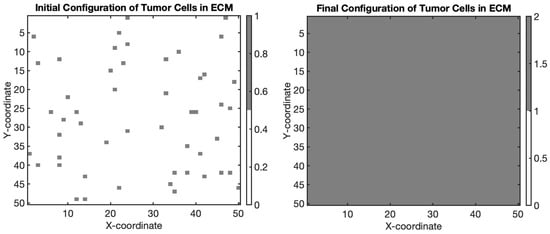
Figure 2.
Simulation of tumor cell migration and proliferation within the extracellular matrix (ECM) using an agent-based model. The gray regions represent tumor cells embedded within the ECM, illustrating their dynamic behavior as they migrate and proliferate within the tissue environment.
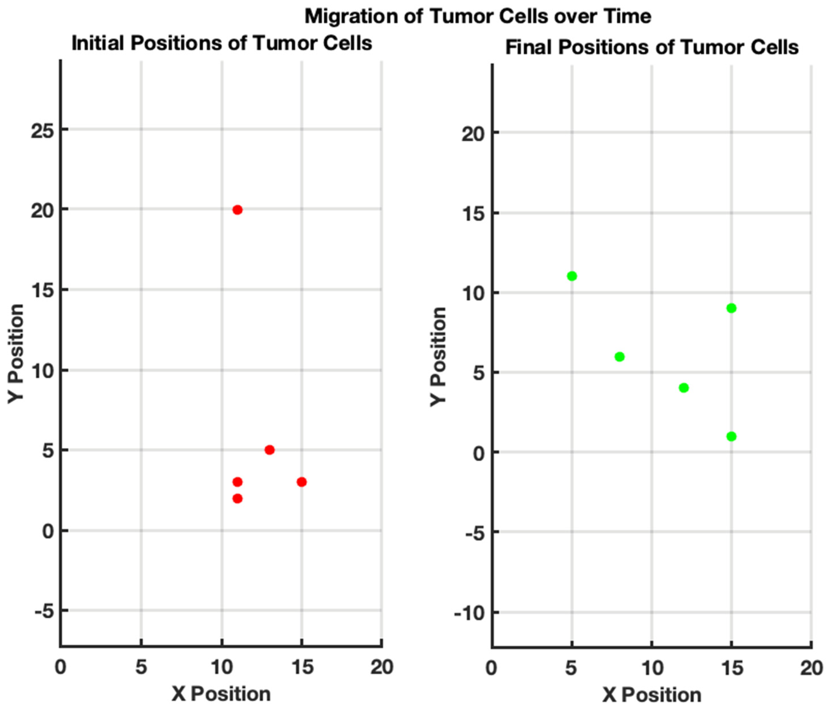
In Figure 3, we have demonstrated the tumor cell migration to simulate the movement of tumor cells within a bounded 20 × 20 grid over a specified number of steps, allowing for a basic representation of random cellular migration. The algorithm begins by initializing parameters, such as the number of tumor cells (5), the total steps for migration (50), and the grid size. Each tumor cell is randomly assigned an initial position within the grid. During each of the 50 steps, the algorithm computes a random direction for each cell to move, introducing variability where cells can either shift one unit in any direction or remain stationary. To ensure that the cells do not migrate outside the designated grid bounds, boundary checks are implemented that readjust any out-of-bound positions back to the nearest edge of the grid. This simple yet effective model captures the essential dynamics of tumor cell behavior, reflecting the randomness typically observed in biological systems while allowing for the visualization of initial and final positions, thereby providing a foundational framework for more complex simulations of tumor growth and migration behaviors in various research contexts.
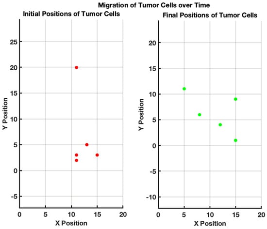
Figure 3.
Migration of tumor cells over time. (Left): initial positions of tumor cells. The scatter plot illustrates the random initial distribution of five tumor cells on a 20 × 20 grid. Each red point represents the starting location of a tumor cell before migration. (Right): final positions of tumor cells after 50 steps of random migration. The scatter plot shows the new positions of the same tumor cells after undergoing 50 steps of random movement within the grid. Each green point indicates the location of a tumor cell following the migration process.
The initial and final configurations of tumor cells within the ECM are visualized in the figures. In the initial configuration, tumor cells are randomly distributed within the matrix environment. Over successive iterations of the agent-based model simulation, tumor cells exhibit dynamic behavior characterized by migration and proliferation.
During each iteration, tumor cells have a probability of migrating to neighboring grid locations, simulating their movement through the ECM. Additionally, tumor cells may proliferate, giving rise to new cells within close proximity. These processes contribute to the spatial evolution of the tumor microenvironment, ultimately impacting tumor growth and invasion dynamics.
In summary, this simulation represents the migration of tumor cells within a defined grid, starting from randomly initialized positions, which represent their initial locations on the grid. Over a series of steps, the tumor cells randomly move in different directions—up, down, left, or right—mimicking the unpredictable nature of cell migration. After completing the designated number of migration steps, the new positions of the tumor cells are visually represented alongside their original locations. This highlights how, despite their initial positions, the cells have migrated to new locations within the grid, illustrating the process of tumor cell movement within a tissue environment. The initial positions are marked in red, while the final positions after the migration are depicted in green, effectively demonstrating the overall shift in location due to migration dynamics. By observing the final configuration of tumor cells, researchers can gain insights into the spatial distribution and density of tumor cells within the ECM, providing valuable information for understanding tumor progression and informing therapeutic interventions targeting the tumor microenvironment.
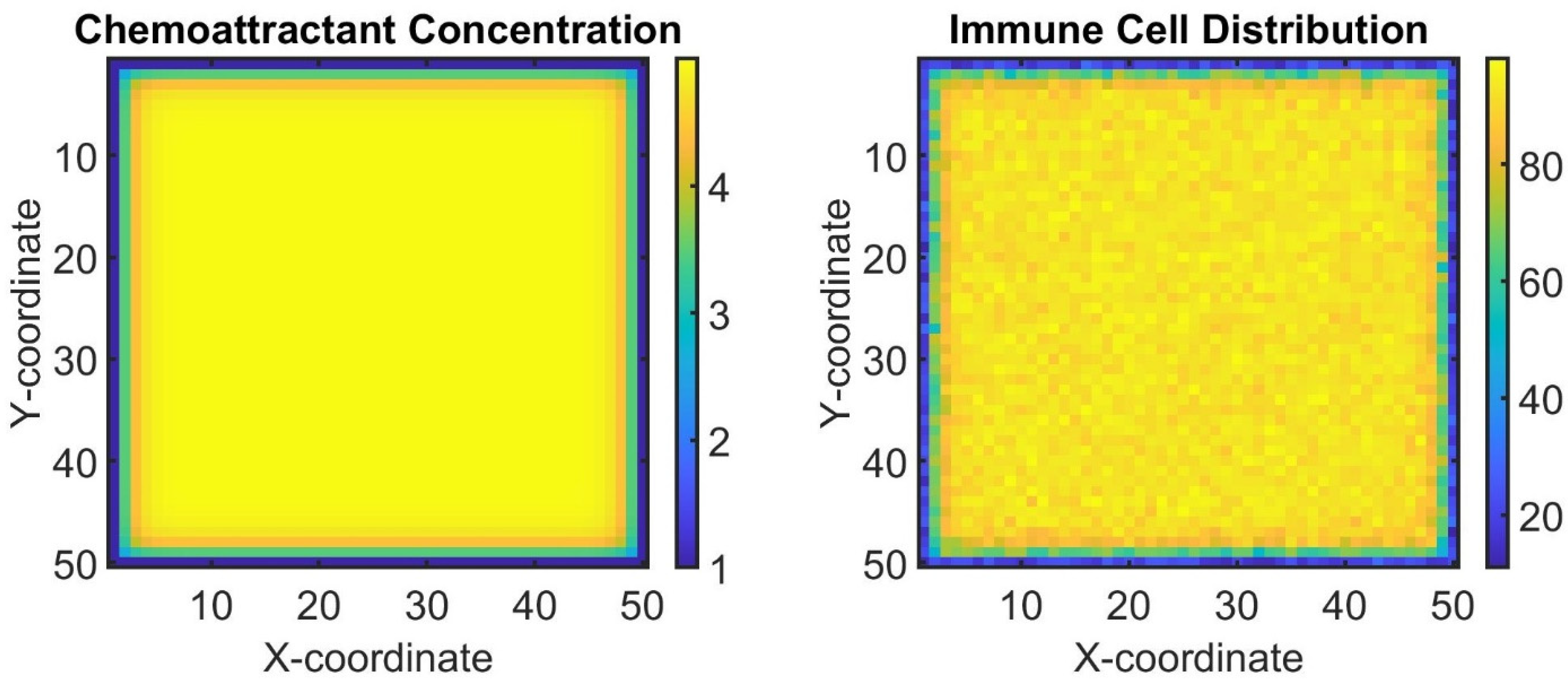
Now we demonstrate another aspect of the tumor microenvironment by modeling the interaction between tumor cells and immune cells. We will simulate a simplified version using a reaction–diffusion model, where tumor cells produce a chemoattractant that recruits immune cells to the tumor site (see Figure 4).
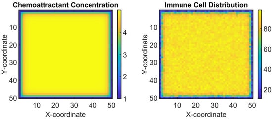
Figure 4.
Simulation of the tumor microenvironment interaction between tumor cells and immune cells using a reaction–diffusion model. (Left): chemoattractant concentration map produced by tumor cells. (Right): distribution of immune cells recruited to the tumor site based on the chemoattractant gradient. The color bar chemo grid plot indicates the concentration of the chemoattractant at different points in the grid. Different color shades represent various levels of concentration, with certain colors indicating higher or lower concentrations. The colors in the immune grid plot reflect the number of immune cells present at each grid point. Different colors represent varying quantities of immune cells, allowing viewers to quickly discern areas of high and low immune cell presence.
Where the biological parameters are defined as follows:
| Diffusion Coefficient | This parameter represents the rate at which chemoattractant molecules diffuse through the tissue. In biological systems, diffusion is driven by the random movement of molecules and is influenced by factors, such as tissue density and viscosity. A higher diffusion coefficient indicates that the chemoattractant spreads more quickly and widely, potentially attracting immune cells from a larger area. In contrast, a lower diffusion coefficient suggests limited spread, focusing the immune response closer to the source of chemoattractant production. |
| Tumor Production Rate | This rate refers to the production of chemoattractant by tumor cells. Tumor cells often secrete various signaling molecules to manipulate the surrounding environment, including attracting immune cells or promoting angiogenesis (the formation of new blood vessels). A higher tumor production rate simulates a more aggressive tumor that releases large amounts of chemoattractant, potentially leading to a stronger and more localized immune response. Conversely, a lower rate represents a less aggressive tumor with weaker signaling. |
| Immune Production Rate | This parameter models the recruitment rate of immune cells in response to the concentration of the chemoattractant. Immune cells are attracted to higher concentrations of chemoattractants, which signal the presence of pathogens or abnormal cells, such as tumor cells. A higher immune production rate means that immune cells are more responsive to the chemoattractant, leading to a rapid accumulation of immune cells in areas with a high chemoattractant concentration. A lower rate indicates a weaker immune response. |
| Decay Rate | This represents the natural degradation or clearance of the chemoattractant over time. In biological systems, molecules can degrade due to enzymatic activity, dilution, or other processes. A higher decay rate means the chemoattractant concentration decreases quickly, reducing its effectiveness over time. This can limit the duration and extent of the immune response. A lower decay rate indicates more persistent chemoattractant signaling. |
These parameters collectively model the complex interactions between tumor cells and the immune system. By adjusting these parameters, researchers can simulate different tumor behaviors and immune responses, providing insights into how tumors evade the immune system or how immune cells can effectively target tumor cells, with the following example:
| Aggressive Tumors | High tumor production rates and low decay rates can simulate aggressive tumors that create a strong and persistent chemoattractant signal, leading to a robust but possibly localized immune response. |
| Weak Immune Responses | Low immune production rates can model scenarios where the immune system is unable to effectively respond to the tumor, which might occur in immunocompromised individuals. |
| Therapeutic Interventions | By manipulating these parameters, researchers can explore potential therapeutic strategies, such as increasing the immune production rate (e.g., through immunotherapy) or reducing the decay rate (e.g., by stabilizing chemoattractants) to enhance the immune response against tumors. |
This figure illustrates the dynamic interaction between tumor cells and immune cells within the tumor microenvironment. In the left subplot, the color map represents the spatial distribution of the chemoattractant produced by tumor cells, which forms a gradient attracting immune cells towards the tumor site. In the right subplot, the distribution of immune cells recruited to the tumor site based on the chemoattractant gradient is depicted. Immune cells are recruited to regions with higher chemoattractant concentrations, reflecting their response to tumor-derived signals within the microenvironment. Overall, this simulation represents a simplified model of the biological interaction between tumor cells and the immune system, highlighting key processes, such as the production and diffusion of signaling molecules and the recruitment of immune cells in response to those signals. It provides a computational framework to examine how local concentrations of chemoattractants can influence the immune environment in the context of cancer biology.
3. Mathematical Oncology of Metastatic Cancer
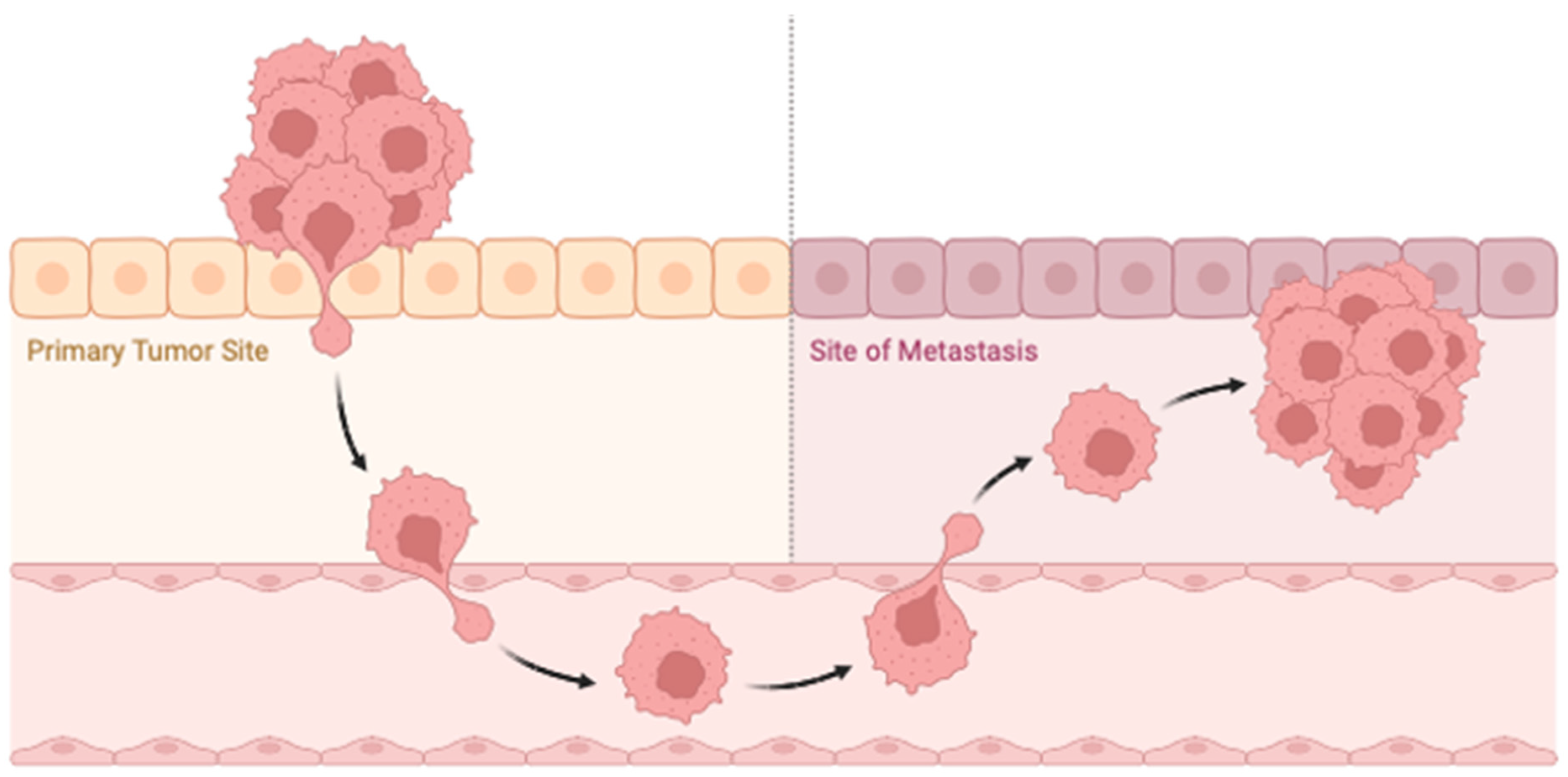
Recent advancements in mathematical oncology have profoundly influenced the study of metastatic cancer, providing critical insights into the mechanisms driving metastasis and the progression of cancer to distant sites (see Figure 5). Contemporary models focus on the dynamics of tumor cell migration, invasion, and colonization in secondary organs, capturing the complex interplay between cancer cells and the microenvironments of both primary and metastatic sites [23,24,25]. These models employ a range of mathematical techniques, including differential equations, agent-based models, and stochastic processes, to simulate the metastatic cascade and predict patient-specific disease progression and treatment outcomes [26,27]. By integrating clinical data, mathematical models are also used to optimize therapeutic strategies, aiming to mitigate metastasis and improve survival rates. These advancements underscore the potential of mathematical oncology to revolutionize our understanding and management of metastatic cancer, paving the way for more effective, personalized interventions [28,29,30,31,32].
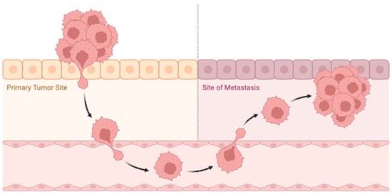
Figure 5.
Schematic representation of metastatic cancer. This schematic illustrates the multi-step process of cancer metastasis, highlighting key stages, including local invasion, intravasation into the bloodstream, circulation through the vascular system, extravasation into distant tissues, and colonization to form secondary tumors. The diagram also depicts the interaction between cancer cells and the tumor microenvironment, including stromal cells, immune cells, and the extracellular matrix, which influence the metastatic process. The figure underscores the complexity of metastatic spread and the critical role of various microenvironmental factors in facilitating cancer progression to distant sites. Figure created using Biorender.
Mathematical modeling equations to describe the impact of interventions on metastatic cancer outcomes involve integrating the effects of treatments on various aspects of tumor growth and progression (see the Algorithm 2). Here is a simplified set of equations to illustrate this. Tumor growth inhibition:
This equation describes the rate of change in tumor volume (V) over time (t). The term represents the logistic growth of the tumor, with r as the tumor growth rate and K as the carrying capacity. The term δ V accounts for the natural death rate of tumor cells, and represents the impact of treatment (VT) on the tumor volume, with α as the treatment efficacy parameter. Metastatic spread inhibition:
Here, M represents the number of metastatic lesions, and the equation describes the rate of change in metastatic lesions over time. The term γ V represents the rate of metastatic spread from the primary tumor, with γ as the metastatic seeding rate.
The term β M accounts for the natural death rate of metastatic lesions, and represents the impact of treatment (MT) on metastatic lesions, with θ as the treatment efficacy parameter. Overall survival:
This equation describes the rate of change in overall survival (S) over time. The term μ S represents the natural death rate of the patient population, and represents the impact of treatment () on overall survival, with σ as the treatment efficacy parameter.
These equations provide a simplified framework for modeling the impact of interventions on metastatic cancer outcomes, including effects on tumor growth, metastatic spread, and overall patient survival. More complex models may incorporate additional factors, such as drug pharmacokinetics, immune system interactions, and tumor heterogeneity to better capture the dynamics of metastatic cancer and the effects of treatments.
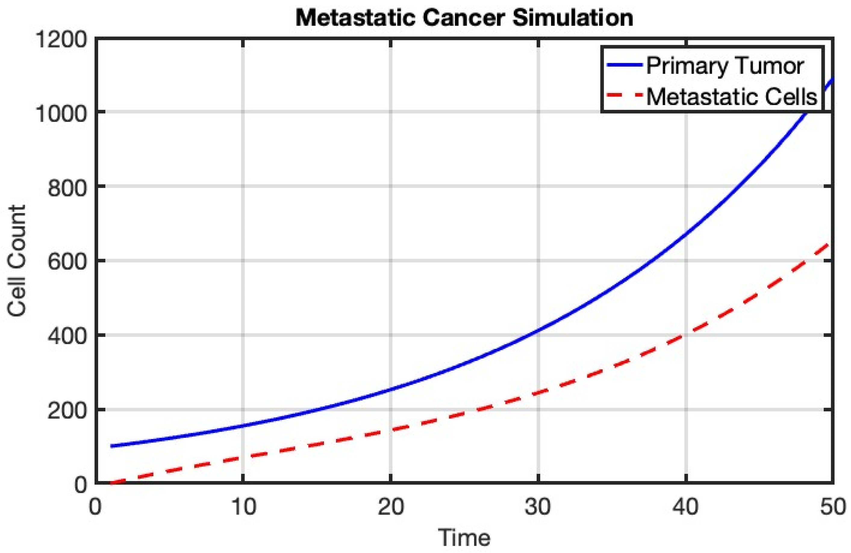
To simulate metastatic cancer, we consider a basic model where we simulate the growth of a primary tumor and the spread of metastatic cells to a secondary site. We will use a simple mathematical model where we simulate tumor growth at the primary site and the dissemination of metastatic cells to the secondary site (see Figure 6).
| Algorithm 2. Tumor Growth and Metastasis |
| Initialize primary_tumor_size with initial_primary_tumor_size |
| Initialize metastatic_cells with initial_metastatic_cells |
| primary_tumor_size(t) = primary_tumor_size(t − 1) + growth_rate_primary_tumor × primary_tumor_size(t − 1) |
| Update metastatic_cells(t): |
| metastatic_cells(t) = metastatic_cells(t − 1) + migration_rate × primary_tumor_size(t − 1) |
| metastatic_cells(t) = survival_rate_metastatic_cells × metastatic_cells(t) |
| initial_primary_tumor_size = 100; % Initial size of the primary tumor |
| initial_metastatic_cells = 0; % Initial number of metastatic cells |
| growth_rate_primary_tumor = 0.05; % Growth rate of the primary tumor |
| migration_rate = 0.1; % Rate of migration of metastatic cells to secondary site |
| survival_rate_metastatic_cells = 0.9; % Survival rate of metastatic cells |
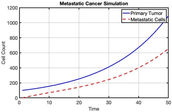
Figure 6.
Simulation of metastatic cancer using a mathematical model. The blue line represents the growth of the primary tumor, while the red dashed line indicates the count of metastatic cells at the secondary site. The model illustrates the progression of cancer from the primary site to distant organs.
Where the biological parameters are listed below:
| Initial Primary Tumor Size | This parameter represents the initial number of cancer cells forming the primary tumor at the start of the simulation. It provides the baseline size from which the tumor will grow. A larger initial primary tumor size indicates a more advanced stage of cancer at the start of the simulation. This can impact the speed at which the tumor reaches clinically significant sizes and begins metastasis. In contrast, a smaller initial size represents an early-stage tumor, possibly still localized and not yet detectable through clinical imaging. |
| Initial Metastatic Cells | This represents the initial number of cancer cells that have already migrated from the primary tumor to a secondary site at the start of the simulation. Typically, this might be zero if the tumor has not yet metastasized. Starting with a nonzero number of metastatic cells can model a scenario where metastasis has already begun, allowing the study of metastatic growth dynamics and the impact of treatments on established metastatic sites. |
| Growth Rate of Primary Tumor | This rate indicates how quickly the primary tumor grows over time. Tumor growth is influenced by factors, such as the rate of cell division, availability of nutrients, and the tumor microenvironment. A higher growth rate represents a more aggressive and rapidly expanding tumor, leading to quicker progression to advanced stages. A lower growth rate indicates a slower-growing tumor, which may remain localized for a longer period. |
| Migration Rate | This parameter models the rate at which cancer cells detach from the primary tumor and migrate to secondary sites (metastasis). Migration can occur through blood vessels (hematogenous spread) or lymphatic vessels (lymphatic spread). A higher migration rate indicates that cancer cells are more likely to spread to other parts of the body, leading to metastasis. This parameter is critical in understanding how quickly a primary tumor can lead to secondary tumor sites, influencing treatment strategies aimed at preventing or slowing metastasis. |
| Survival Rate of Metastatic Cells | This rate represents the likelihood of metastatic cells surviving and establishing a secondary tumor at a new site. The survival of metastatic cells depends on their ability to adapt to the new microenvironment, evade the immune response, and establish a blood supply. A higher survival rate suggests that metastatic cells are more likely to thrive and grow into secondary tumors, contributing to the spread of cancer. Lower survival rates indicate a reduced likelihood of successful metastasis, which can be targeted by therapies that make secondary sites less hospitable for migrating cancer cells. |
These parameters collectively model the critical aspects of cancer progression, from the initial growth of the primary tumor to the spread and establishment of metastatic sites. By adjusting these parameters, researchers can simulate different cancer behaviors and responses to treatment:
| Aggressive Tumors | High growth rates for the primary tumor and high migration and survival rates for metastatic cells can simulate highly aggressive cancers, leading to rapid progression and widespread metastasis. Such simulations can help in understanding the behavior of fast-growing cancers and the urgency required in treatment. |
| Slow-Growing Tumors | Lower growth rates and migration rates can model indolent cancers that grow slowly and are less likely to metastasize. These simulations can be used to study cancers that may be managed with watchful waiting or less aggressive treatments. |
| Therapeutic Interventions | By manipulating parameters, such as the growth rate (e.g., through chemotherapy) or the migration and survival rates of metastatic cells (e.g., through targeted therapies or immunotherapy), researchers can explore the potential impact of different treatment strategies. This can help in designing effective treatment plans that slow down tumor growth, prevent metastasis, or reduce the survival of metastatic cells. |
This figure illustrates the dynamics of metastatic cancer, simulated using a mathematical model. The blue line represents the growth of the primary tumor at the primary site, following a growth rate defined by the model parameters. The red dashed line indicates the count of metastatic cells at a secondary site, which increases over time due to migration from the primary tumor and is subject to a survival rate. This simulation provides insights into the progression of cancer and the spread of metastatic cells to distant organs, highlighting the importance of understanding and targeting metastasis in cancer treatment.
4. Discussion
Cancer, a multifaceted disease characterized by uncontrolled cell growth and metastasis, presents a formidable challenge due to its inherent complexity and heterogeneity. Traditional research approaches often struggle to capture the intricate interplay between various biological processes within the tumor microenvironment. Mathematical modeling emerges as a powerful tool in this domain, offering a quantitative framework to analyze and predict tumor behavior. One key application of mathematical modeling lies in understanding tumor growth and angiogenesis. By incorporating factors like cell proliferation, death, and nutrient availability, population dynamics models can simulate tumor growth kinetics and predict potential responses to therapeutic interventions. Additionally, spatial models can further account for diffusion and reaction kinetics, providing insights into how physical factors, like nutrient and oxygen gradients, influence tumor development and metastasis.
Mathematical oncology goes beyond tumor growth, delving deeper into the complex ecosystem of the tumor microenvironment. This microenvironment, composed of cancer cells, immune cells, stromal cells, and extracellular matrix, significantly influences tumor behavior. Mathematical models can be employed to investigate how interactions within this microenvironment contribute to tumor growth, invasion, and treatment resistance. By capturing the dynamic interplay between these cellular and molecular components, these models offer insights into the mechanisms underlying cancer progression and pave the way for the development of targeted therapies. The power of mathematical modeling extends to understanding the evolution of cancer cells. By incorporating evolutionary principles, models can simulate the process of clonal expansion, diversification, and selection within tumors. This exploration helps to elucidate how genetic and phenotypic variations arise, leading to the emergence of drug-resistant subclones and the potential for metastasis. Understanding these evolutionary dynamics is crucial for developing effective therapeutic strategies that can target and eliminate diverse tumor cell populations. Furthermore, mathematical modeling plays a pivotal role in personalized medicine. By integrating patient-derived data, such as genomic profiles and imaging information, with computational models, clinicians can develop individualized treatment plans that maximize efficacy and minimize adverse effects. This approach holds the promise of revolutionizing cancer care by tailoring therapies to the unique genetic and clinical profile of each patient.
Challenges and Opportunities in Mathematical Oncology:
While mathematical modeling holds immense promise for advancing our understanding of cancer, several key challenges must be addressed to fully realize its potential. The inherent complexity of biological systems, coupled with the heterogeneity of tumors, necessitates the development of sophisticated models capable of capturing the intricate interplay of various factors influencing cancer progression.
Data availability and quality pose significant challenges in model development. Comprehensive and accurate data, including clinical, genomic, and imaging information, are essential for building robust models. However, obtaining high-quality data that are representative of the patient population can be difficult. Additionally, integrating data from multiple sources and ensuring data consistency is a complex task.
Model validation and uncertainty quantification are critical steps in ensuring the reliability of mathematical models. Validating models against experimental data and clinical outcomes is essential to establish their credibility. However, the complexity of biological systems often makes it challenging to definitively validate models. Incorporating uncertainty quantification into model predictions can help to assess the robustness of model outputs and inform decision-making.
Translating mathematical models into clinical practice requires overcoming several hurdles. Developing user-friendly software tools and establishing standardized protocols for model implementation are essential for widespread adoption. Furthermore, educating clinicians about the potential benefits and limitations of mathematical modeling is crucial for building trust and facilitating its integration into clinical workflows. Despite these challenges, the future of mathematical oncology is bright. Advancements in computational power, data science, and artificial intelligence offer new opportunities to address these limitations. By developing more sophisticated algorithms, incorporating larger and more diverse datasets, and fostering interdisciplinary collaborations, researchers can create increasingly accurate and predictive models. Ultimately, the goal of mathematical oncology is to improve patient outcomes through the development of personalized and effective cancer therapies. By addressing the challenges and capitalizing on emerging opportunities, this field has the potential to transform cancer care.
5. Conclusions
Mathematical oncology has emerged as a critical discipline in the complex landscape of cancer research. By providing a quantitative framework to analyze and predict tumor behavior, this field has significantly advanced our understanding of cancer initiation, progression, and treatment responses. Through the integration of biological, physical, and mathematical principles, mathematical oncology offers a holistic perspective on cancer, enabling researchers to unravel the intricate mechanisms underlying this multifaceted disease. From simulating tumor growth patterns to exploring the dynamics of the tumor microenvironment, mathematical models have become indispensable tools for elucidating cancer biology. These models have not only enhanced our understanding of fundamental cancer processes but have also informed the development of novel therapeutic strategies. The ability to predict treatment responses, optimize clinical trial designs, and personalize cancer care underscores the transformative potential of mathematical oncology. The synergy between experimental and computational approaches is essential for advancing the field. By combining large-scale data generation with sophisticated modeling techniques, researchers can uncover hidden patterns, identify novel therapeutic targets, and accelerate the drug discovery process. As computational power and data availability continue to expand, mathematical oncology is poised to play an even more critical role in reshaping cancer care. Ultimately, the integration of mathematical modeling into cancer research holds the promise of improving patient outcomes and saving lives. By fostering interdisciplinary collaborations and investing in computational infrastructure, we can harness the full potential of mathematical oncology to address this global health challenge.
Funding
This research received no external funding.
Data Availability Statement
No new data were created or analyzed in this study.
Conflicts of Interest
The author declares no conflict of interest.
References
- Anderson, A.R.; Weaver, A.M.; Cummings, P.T.; Quaranta, V. Tumor morphology and phenotypic evolution driven by selective pressure from the microenvironment. Cell 2006, 127, 905–915. [Google Scholar] [CrossRef] [PubMed]
- Murray, J. An Introduction; Springer: New York, NY, USA, 2002. [Google Scholar]
- Chaplain, M.A.J.; Anderson, A.R.A. Mathematical modeling of tumor-induced angiogenesis. Annu. Rev. Biomed. Eng. 2011, 3, 219–241. [Google Scholar]
- Azizi, T. Intersections of Neurobiology and Oncology: Foundations and Frontiers in Cancer Neuroscience; BP International: Hong Kong, China, 2024. [Google Scholar]
- Azizi, T. Mathematical Modeling with Applications in Biological Systems, Physiology, and Neuroscience. Ph.D. Thesis, Kansas State University, Manhattan, KS, USA, 2021. [Google Scholar]
- Azizi, T.; Mugabi, R. Global sensitivity analysis in physiological systems. Appl. Math. Sci. Res. Publ. 2020, 11, 119–136. [Google Scholar] [CrossRef]
- Byrne, H.M. Dissecting cancer through mathematics: From the cell to the animal model. Nat. Rev. Cancer 2010, 10, 221–230. [Google Scholar] [CrossRef]
- Gatenby, R.A.; Silva, A.S.; Gillies, R.J.; Frieden, B.R. Adaptive therapy. Cancer Res. 2009, 69, 4894–4903. [Google Scholar] [CrossRef]
- Foo, J.; Michor, F. Evolution of resistance to targeted anti-cancer therapies during continuous and pulsed administration strategies. PLoS Comput Biol. 2009, 5, e1000557. [Google Scholar] [CrossRef]
- Araujo, R.P.; McElwain, D.L.S. A history of the study of solid tumour growth: The contribution of mathematical modelling. Bull. Math. Biol. 2004, 66, 1039–1091. [Google Scholar] [CrossRef] [PubMed]
- Swanson, K.R.; Rockne, R.C.; Claridge, J.; Chaplain, M.A.J.; Alvord, E.C.; Anderson, A.R.A. Quantifying the role of angiogenesis in malignant progression of gliomas: In silico modeling integrates imaging and histology. Cancer Res. 2011, 71, 7366–7737. [Google Scholar] [CrossRef]
- De Pillis, L.G.; Radunskaya, A.E. A mathematical tumor model with immune resistance and drug therapy: An optimal control approach. Comput. Math. Methods Med. 2001, 3, 79–100. [Google Scholar] [CrossRef]
- Kirschner, D.; Panetta, J.C. Modeling immunotherapy of the tumor–immune interaction. J. Math. Biol. 1998, 37, 235–252. [Google Scholar] [CrossRef]
- Galluzzi, L.; Vacchelli, E.; Bravo-San Pedro, J.M.; Buqué, A.; Senovilla, L.; Baracco, E.E.; Bloy, N.; Castoldi, F.; Abastado, J.-P.; Agostinis, P.; et al. Classification of current anticancer immunotherapies. Oncotarget 2014, 5, 12472. [Google Scholar] [CrossRef]
- Restifo, N.P.; Dudley, M.E.; Rosenberg, S.A. Adoptive immunotherapy for cancer: Harnessing the T cell response. Nat. Rev. Immunol. 2012, 12, 269–281. [Google Scholar] [CrossRef] [PubMed]
- Norton, L. A Gompertzian model of human breast cancer growth. Cancer Res. 1988, 48, 7067–7071. [Google Scholar] [PubMed]
- Panetta, J.C. A mathematical model of breast and ovarian cancer treated with paclitaxel. Math. Biosci. 1997, 146, 89–113. [Google Scholar] [CrossRef]
- Foo, J.; Leder, K.; Michor, F. Stochastic dynamics of cancer initiation. Phys. Biol. 2011, 8, 015002. [Google Scholar] [CrossRef] [PubMed]
- Schättler, H.; Ledzewicz, U. Optimal Control for Mathematical Models of Cancer Therapies. An Application of Geometric Methods; Springer: Berlin/Heidelberg, Germany, 2015. [Google Scholar]
- Enderling, H.; Hlatky, L.; Hahnfeldt, P. Cancer stem cells: A minor cancer subpopulation that redefines global cancer features. Front. Oncol. 2013, 3, 76. [Google Scholar] [CrossRef]
- Gatenby, R.A.; Gawlinski, E.T.; Gmitro, A.F.; Kaylor, B.; Gillies, R.J. Acid-mediated tumor invasion: A multidisciplinary study. Cancer Res. 2006, 66, 5216–5223. [Google Scholar] [CrossRef]
- Anderson, A.R.A.; Quaranta, V. Integrative mathematical oncology. Nat. Rev. Cancer 2008, 8, 227–234. [Google Scholar] [CrossRef]
- Masuda, N.; Petter, H. Predicting and controlling infectious disease epidemics using temporal networks. F1000Prime Rep. 2013, 5, 6. [Google Scholar] [CrossRef]
- Mahlbacher, G.E.; Reihmer, K.C.; Frieboes, H.B. Frieboes. Mathematical modeling of tumor-immune cell interactions. J. Theor. Biol. 2019, 469, 47–60. [Google Scholar] [CrossRef]
- Chen, H.; Cai, Y.; Chen, Q.; Li, Z. Multiscale modeling of solid stress and tumor cell invasion in response to dynamic mechanical microenvironment. Biomech. Model. Mechanobiol. 2020, 19, 577–590. [Google Scholar] [CrossRef]
- Valentinuzzi, D.; Jeraj, R. Computational modelling of modern cancer immunotherapy. Phys. Med. Biol. 2020, 65, 24TR01. [Google Scholar] [CrossRef]
- Huang, J.; Zhang, L.; Wan, D.; Zhou, L.; Zheng, S.; Lin, S.; Qiao, Y. Extracellular matrix and its therapeutic potential for cancer treatment. Signal Transduct. Target. Ther. 2021, 6, 153. [Google Scholar] [CrossRef]
- Yankeelov, T.E.; An, G.; Saut, O.; Luebeck, E.G.; Popel, A.S.; Ribba, B.; Vicini, P.; Zhou, X.; Weis, J.A.; Ye, K.; et al. Multi-scale modeling in clinical oncology: Opportunities and barriers to success. Ann. Biomed. Eng. 2016, 44, 2626–2641. [Google Scholar] [CrossRef]
- Surendran, A.; Jenner, A.L.; Karimi, E.; Fiset, B.; Quail, D.F.; Walsh, L.A.; Craig, M. Agent-based modelling reveals the role of the tumor microenvironment on the short-term success of combination temozolomide/immune checkpoint blockade to treat glioblastoma. J. Pharmacol. Exp. Ther. 2023, 387, 66–77. [Google Scholar] [CrossRef]
- Franssen, L.C.; Lorenzi, T.; Burgess, A.E.; Chaplain, M.A. A mathematical framework for modelling the metastatic spread of cancer. Bull. Math. Biol. 2019, 81, 1965–2010. [Google Scholar] [CrossRef]
- Szczurek, E.; Krüger, T.; Klink, B.; Beerenwinkel, N. A mathematical model of the metastatic bottleneck predicts patient outcome and response to cancer treatment. PLoS Comput. Biol. 2020, 16, e1008056. [Google Scholar] [CrossRef]
- Anvari, S.; Nambiar, S.; Pang, J.; Maftoon, N. Computational models and simulations of cancer metastasis. Arch. Comput. Methods Eng. 2021, 28, 4837–4859. [Google Scholar] [CrossRef]

Disclaimer/Publisher’s Note: The statements, opinions and data contained in all publications are solely those of the individual author(s) and contributor(s) and not of MDPI and/or the editor(s). MDPI and/or the editor(s) disclaim responsibility for any injury to people or property resulting from any ideas, methods, instructions or products referred to in the content. |
© 2024 by the author. Licensee MDPI, Basel, Switzerland. This article is an open access article distributed under the terms and conditions of the Creative Commons Attribution (CC BY) license (https://creativecommons.org/licenses/by/4.0/).