
Train Neural Networks with a Hybrid Method That Incorporates a Novel Simulated Annealing Procedure


Abstract
1. Introduction
2. The Proposed Method
2.1. The New Simulated Annealing Variant
| Algorithm 1 The used variant of the Simulated Annealing algorithm. |
procedure siman
|
2.2. The Overall Algorithm
- Initialization Step
- (a)
- Define as the number of chromosomes and as the maximum number of generations.
- (b)
- Define the selection rate and the mutation rate with and .
- (c)
- Set as the number of generations passed before the modified Simulated Algorithm will be applied.
- (d)
- Set as the number of chromosomes that will be altered by the modified Simulated Annealing algorithm.
- (e)
- Perform a random initialization of the chromosomes. Each chromosome represents a different set of randomly initialized weights for the neural network.
- (f)
- Set .
- For each chromosome
- (a)
- Formulate a neural network
- (b)
- Calculate the fitness of chromosome and for the given dataset.
- Genetic operations step
- (a)
- Selection procedure. The chromosomes are sorted with respect to the associated fitness values. The first chromosomes having the lowest fitness values are copied to the next generation. The rest of the chromosomes are replaced by offspings produced in the crossover procedure.
- (b)
- Crossover procedure: In the crossover procedure, pairs of chromosomes are selected from the population using tournament selection. For each pair of selected parents two new chromosomes and are formulated using the following schemewhere . The randomly selected values are chosen in the range [72].
- (c)
- Mutation procedure:
- For each chromosome , conduct the following steps:
- For every element of , a random number is produced. The corresponding element is altered randomly if .
- EndFor
- Local method step
- (a)
- If then
- For do
- Select a random chromosome
- Apply the siman algorithm: of Section 2.1.
- EndFor
- (b)
- Endif
- Termination Check Step
- (a)
- Set
- (b)
- If then goto Termination Step, else goto 2b.
- Termination step
- (a)
- Denote as the chromosome with the lowest fitness value.
- (b)
- Formulate the neural network
- (c)
- Apply a local search procedure to . The local search method used in the current work is a BFGS variant of Powell [73].
- (d)
- Apply the neural network on the test of the objective problem and report the result.
3. Results
- The UCI dataset repository, https://archive.ics.uci.edu/ml/index.php (accessed on 18 June 2024) [74].
- The Keel repository, https://sci2s.ugr.es/keel/datasets.php (accessed on 18 June 2024) [75].
- The Statlib URL http://lib.stat.cmu.edu/datasets/ (accessed on 18 June 2024).
3.1. Classification Datasets
- Appendictis a medical dataset, suggested in [76].
- Australian dataset [77], used in credit card transactions.
- Bands dataset, used to detect printing problems.
- Balance dataset [78], which is related to some psychological experiments.
- Circular dataset, which is an artificial dataset.
- Dermatology dataset [81], which is a dataset related to dermatological deceases.
- Ecoli dataset, a dataset about protein localization sites of proteins [82].
- Fert dataset. Fertility dataset related to relation of sperm concentration and demographic data.
- Heart dataset [83], a medical dataset used to detect heart diseases.
- HeartAttack dataset, used to predict heart attacks.
- HouseVotes dataset [84], related to votes in the U.S. House of Representatives.
- Liverdisorder dataset [85], used to detect liver disorders.
- Parkinsons dataset, used to detect the Parkinson’s disease (PD) [86].
- Pima dataset [87], a medical dataset used to detect the presence of diabetes.
- Popfailures dataset [88], a dataset related to climate measurements.
- Regions2 dataset, related to hepatitis C [89].
- Saheart dataset [90], used to detect heart diseases.
- Segment dataset [91], used in image processing tasks.
- Sonar dataset [92], used to discriminate sonar signals.
- Spiral dataset, an artificial dataset.
- Wdbc dataset [93], a medical dataset used to detect cancer..
- Eeg datasets, a dataset related to EEG measurements [96] and the following cases were used: Z_F_S, ZO_NF_S and ZONF_S.
- Zoo dataset [97], used to classify animals in seven predefined categories.
3.2. Regression Datasets
- Airfoil dataset, a dataset provided by NASA [98].
- BK dataset [99], used for points prediction in a basketball game.
- BL dataset, it contains measurements from an experiment related to electricity.
- Baseball dataset, used to calculate the income of baseball players.
- Dee dataset, used to calculate the price of electricity.
- EU, downloaded from the STALIB repository.
- FY, This dataset measures the longevity of fruit flies.
- HO dataset, downloaded from the STALIB repository.
- Housing dataset, mentioned in [100].
- LW dataset, related to risk factors associated with low weight babies.
- MORTGAGE dataset, related to economic data from USA.
- MUNDIAL, provided from the STALIB repository.
- PL dataset, provided from the STALIB repository.
- QUAKE dataset, that is used to measure the strength of a earthquake.
- REALESTATE, provided from the STALIB repository.
- SN dataset. It contains measurements from an experiment related to trellising and pruning.
- Treasury dataset, related to economic data from USA.
- VE dataset, provided from the STALIB repository.
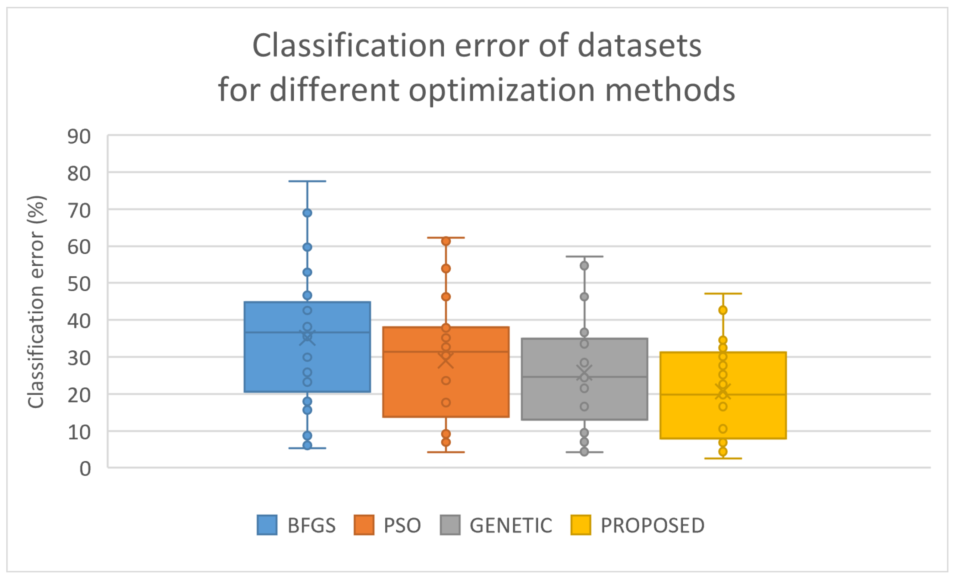
3.3. Experimental Results
- The column DATASET denotes the name of the used dataset.
- The column BFGS denotes the application of the BFGS optimization method to train a neural network with H processing nodes. The method used here is the BFGS variant of Powell [73].
- The column PSO denotes the application of a Particle Swarm Optimizer with particles to train a neural network with H processing nodes. In the current work the improved PSO method, as suggested by Charilogis and Tsoulos, is used [101].
- The column PROPOSED denotes the application of the proposed method, with the parameters of Table 1 on a neural network with H hidden nodes.
- The row AVERAGE denotes the average classification or regression error for all datasets.
4. Conclusions
- Periodic application of an intelligent stochastic technique based on Simulated Annealing. This technique improves the training error of randomly selected chromosomes.
- By using parameters, the changes that this stochastic method can cause in the chromosomes are controlled.
- This stochastic technique can be used without modification in both classification and data fitting problems.
Author Contributions
Funding
Institutional Review Board Statement
Informed Consent Statement
Data Availability Statement
Acknowledgments
Conflicts of Interest
References
- Bishop, C. Neural Networks for Pattern Recognition; Oxford University Press: Oxford, UK, 1995. [Google Scholar]
- Cybenko, G. Approximation by superpositions of a sigmoidal function. Math. Control Signals Syst. 1989, 2, 303–314. [Google Scholar] [CrossRef]
- Baldi, P.; Cranmer, K.; Faucett, T.; Sadowski, P.; Whiteson, D. Parameterized neural networks for high-energy physics. Eur. Phys. J. C 2016, 76, 235. [Google Scholar] [CrossRef]
- Valdas, J.J.; Bonham-Carter, G. Time dependent neural network models for detecting changes of state in complex processes: Applications in earth sciences and astronomy. Neural Netw. 2006, 19, 196–207. [Google Scholar] [CrossRef]
- Carleo, G.; Troyer, M. Solving the quantum many-body problem with artificial neural networks. Science 2017, 355, 602–606. [Google Scholar] [CrossRef]
- Shen, L.; Wu, J.; Yang, W. Multiscale Quantum Mechanics/Molecular Mechanics Simulations with Neural Networks. J. Chem. Theory Comput. 2016, 12, 4934–4946. [Google Scholar] [CrossRef] [PubMed]
- Manzhos, S.; Dawes, R.; Carrington, T. Neural network-based approaches for building high dimensional and quantum dynamics-friendly potential energy surfaces. Int. J. Quantum Chem. 2015, 115, 1012–1020. [Google Scholar] [CrossRef]
- Wei, J.N.; Duvenaud, D.; Aspuru-Guzik, A. Neural Networks for the Prediction of Organic Chemistry Reactions. ACS Cent. Sci. 2016, 2, 725–732. [Google Scholar] [CrossRef] [PubMed]
- Falat, L.; Pancikova, L. Quantitative Modelling in Economics with Advanced Artificial Neural Networks. Procedia Econ. Financ. 2015, 34, 194–201. [Google Scholar] [CrossRef]
- Namazi, M.; Shokrolahi, A.; Sadeghzadeh Maharluie, M. Detecting and ranking cash flow risk factors via artificial neural networks technique. J. Bus. Res. 2016, 69, 1801–1806. [Google Scholar] [CrossRef]
- Tkacz, G. Neural network forecasting of Canadian GDP growth. Int. J. Forecast. 2001, 17, 57–69. [Google Scholar] [CrossRef]
- Baskin, I.I.; Winkler, D.; Tetko, I.V. A renaissance of neural networks in drug discovery. Expert Opin. Drug Discov. 2016, 11, 785–795. [Google Scholar] [CrossRef]
- Bartzatt, R. Prediction of Novel Anti-Ebola Virus Compounds Utilizing Artificial Neural Network (ANN). Chem. Fac. 2018, 49, 16–34. [Google Scholar]
- Kia, M.B.; Pirasteh, S.; Pradhan, B.; Mahmud, A.R. An artificial neural network model for flood simulation using GIS: Johor River Basin, Malaysia. Environ. Earth Sci. 2012, 67, 251–264. [Google Scholar] [CrossRef]
- Yadav, A.K.; Chandel, S.S. Solar radiation prediction using Artificial Neural Network techniques: A review. Renew. Sustain. Energy Rev. 2014, 33, 772–781. [Google Scholar] [CrossRef]
- Getahun, M.A.; Shitote, S.M.; Zachary, C. Artificial neural network based modelling approach for strength prediction of concrete incorporating agricultural and construction wastes. Constr. Build. Mater. 2018, 190, 517–525. [Google Scholar] [CrossRef]
- Chen, M.; Challita, U.; Saad, W.; Yin, C.; Debbah, M. Artificial Neural Networks-Based Machine Learning for Wireless Networks: A Tutorial. IEEE Commun. Surv. Tutor. 2019, 21, 3039–3071. [Google Scholar] [CrossRef]
- Peta, K.; Żurek, J. Prediction of air leakage in heat exchangers for automotive applications using artificial neural networks. In Proceedings of the 2018 9th IEEE Annual Ubiquitous Computing, Electronics & Mobile Communication Conference (UEMCON), New York, NY, USA, 8–10 November 2018; pp. 721–725. [Google Scholar]
- Tsoulos, I.G.; Gavrilis, D.; Glavas, E. Neural network construction and training using grammatical evolution. Neurocomputing 2008, 72, 269–277. [Google Scholar] [CrossRef]
- Guarnieri, S.; Piazza, F.; Uncini, A. Multilayer feedforward networks with adaptive spline activation function. IEEE Trans. Neural Netw. 1999, 10, 672–683. [Google Scholar] [CrossRef]
- Ertuğrul, Ö.F. A novel type of activation function in artificial neural networks: Trained activation function. Neural Netw. 2018, 99, 148–157. [Google Scholar] [CrossRef]
- Rasamoelina, A.D.; Adjailia, F.; Sinčák, P. A Review of Activation Function for Artificial Neural Network. In Proceedings of the 2020 IEEE 18th World Symposium on Applied Machine Intelligence and Informatics (SAMI), Herlany, Slovakia, 23–25 January 2010; pp. 281–286. [Google Scholar]
- Rumelhart, D.E.; Hinton, G.E.; Williams, R.J. Learning representations by back-propagating errors. Nature 1986, 323, 533–536. [Google Scholar] [CrossRef]
- Chen, T.; Zhong, S. Privacy-Preserving Backpropagation Neural Network Learning. IEEE Trans. Neural Netw. 2009, 20, 1554–1564. [Google Scholar] [CrossRef] [PubMed]
- Wilamowski, B.M.; Iplikci, S.; Kaynak, O.; Efe, M.O. An algorithm for fast convergence in training neural network. In Proceedings of the IJCNN’01. International Joint Conference on Neural Networks. Proceedings (Cat. No.01CH37222), Washington, DC, USA, 15–19 July 2001; Volume 3, pp. 1778–1782. [Google Scholar] [CrossRef]
- Riedmiller, M.; Braun, H. A Direct Adaptive Method for Faster Backpropagation Learning: The RPROP algorithm. In Proceedings of the the IEEE International Conference on Neural Networks, San Francisco, CA, USA, 28 March–1 April 1993; pp. 586–591. [Google Scholar]
- Pajchrowski, T.; Zawirski, K.; Nowopolski, K. Neural Speed Controller Trained Online by Means of Modified RPROP Algorithm. IEEE Trans. Ind. Inform. 2015, 11, 560–568. [Google Scholar] [CrossRef]
- Hermanto, R.P.S.; Suharjito; Diana; Nugroho, A. Waiting-Time Estimation in Bank Customer Queues using RPROP Neural Networks. Procedia Comput. Sci. 2018, 135, 35–42. [Google Scholar] [CrossRef]
- Robitaille, B.; Marcos, B.; Veillette, M.; Payre, G. Modified quasi-Newton methods for training neural networks. Comput. Chem. Eng. 1996, 20, 1133–1140. [Google Scholar] [CrossRef]
- Liu, Q.; Liu, J.; Sang, R.; Li, J.; Zhang, T.; Zhang, Q. Fast Neural Network Training on FPGA Using Quasi-Newton Optimization Method. IEEE Trans. Very Large Scale Integr. (Vlsi) Syst. 2018, 26, 1575–1579. [Google Scholar] [CrossRef]
- Zhang, C.; Shao, H.; Li, Y. Particle swarm optimisation for evolving artificial neural network. In Proceedings of the IEEE International Conference on Systems, Man, and Cybernetics, Nashville, TN, USA, 8–11 October 200; pp. 2487–2490.
- Yu, J.; Wang, S.; Xi, L. Evolving artificial neural networks using an improved PSO and DPSO. Neurocomputing 2008, 71, 1054–1060. [Google Scholar] [CrossRef]
- Ilonen, J.; Kamarainen, J.K.; Lampinen, J. Differential Evolution Training Algorithm for Feed-Forward Neural Networks. Neural Process. Lett. 2003, 17, 93–105. [Google Scholar] [CrossRef]
- Zhang, L.; Suganthan, P.N. A survey of randomized algorithms for training neural networks. Inf. Sci. 2016, 364–365, 146–155. [Google Scholar] [CrossRef]
- Yaghini, M.; Khoshraftar, M.M.; Fallahi, M. A hybrid algorithm for artificial neural network training. Eng. Appl. Artif. Intell. 2013, 26, 293–301. [Google Scholar] [CrossRef]
- Chen, J.F.; Do, Q.H.; Hsieh, H.N. Training Artificial Neural Networks by a Hybrid PSO-CS Algorithm. Algorithms 2015, 8, 292–308. [Google Scholar] [CrossRef]
- Yang, X.S.; Deb, S. Engineering Optimisation by Cuckoo Search. Int. J. Math. Model. Numer. Optim. 2010, 1, 330–343. [Google Scholar] [CrossRef]
- Ivanova, I.; Kubat, M. Initialization of neural networks by means of decision trees. Knowl.-Based Syst. 1995, 8, 333–344. [Google Scholar] [CrossRef]
- Yam, J.Y.F.; Chow, T.W.S. A weight initialization method for improving training speed in feedforward neural network. Neurocomputing 2000, 30, 219–232. [Google Scholar] [CrossRef]
- Chumachenko, K.; Iosifidis, A.; Gabbouj, M. Feedforward neural networks initialization based on discriminant learning. Neural Netw. 2022, 146, 220–229. [Google Scholar] [CrossRef] [PubMed]
- Narkhede, M.V.; Bartakke, P.P.; Sutaone, M.S. A review on weight initialization strategies for neural networks. Artif. Intell. Rev. 2022, 55, 291–322. [Google Scholar] [CrossRef]
- Oh, K.-S.; Jung, K. GPU implementation of neural networks. Pattern Recognit. 2004, 37, 1311–1314. [Google Scholar] [CrossRef]
- Huqqani, A.A.; Schikuta, E.; Ye, S.; Chen, P. Multicore and GPU Parallelization of Neural Networks for Face Recognition. Procedia Comput. Sci. 2013, 18, 349–358. [Google Scholar] [CrossRef]
- Zhang, M.; Hibi, K.; Inoue, J. GPU-accelerated artificial neural network potential for molecular dynamics simulation. Comput. Commun. 2023, 285, 108655. [Google Scholar] [CrossRef]
- Pallipuram, V.K.; Bhuiyan, M.; Smith, M.C. A comparative study of GPU programming models and architectures using neural networks. J. Supercomput. 2012, 61, 673–718. [Google Scholar] [CrossRef]
- Holland, J.H. Genetic algorithms. Sci. Am. 1992, 267, 66–73. [Google Scholar] [CrossRef]
- Stender, J. Parallel Genetic Algorithms: Theory & Applications; IOS Press: Amsterdam, The Netherlands, 1993. [Google Scholar]
- Goldberg, D. Genetic Algorithms in Search, Optimization and Machine Learning; Addison-Wesley Publishing Company: Reading, MA, USA, 1989. [Google Scholar]
- Michaelewicz, Z. Genetic Algorithms + Data Structures = Evolution Programs; Springer: Berlin/Heidelberg, Germany, 1996. [Google Scholar]
- Santana, Y.H.; Alonso, R.M.; Nieto, G.G.; Martens, L.; Joseph, W.; Plets, D. Indoor genetic algorithm-based 5G network planning using a machine learning model for path loss estimation. Appl. Sci. 2022, 12, 3923. [Google Scholar] [CrossRef]
- Liu, X.; Jiang, D.; Tao, B.; Jiang, G.; Sun, Y.; Kong, J.; Chen, B. Genetic algorithm-based trajectory optimization for digital twin robots. Front. Bioeng. Biotechnol. 2022, 9, 793782. [Google Scholar] [CrossRef] [PubMed]
- Nonoyama, K.; Liu, Z.; Fujiwara, T.; Alam, M.M.; Nishi, T. Energy-efficient robot configuration and motion planning using genetic algorithm and particle swarm optimization. Energies 2022, 15, 2074. [Google Scholar] [CrossRef]
- Liu, K.; Deng, B.; Shen, Q.; Yang, J.; Li, Y. Optimization based on genetic algorithms on energy conservation potential of a high speed SI engine fueled with butanol–gasoline blends. Energy Rep. 2022, 8, 69–80. [Google Scholar] [CrossRef]
- Zhou, G.; Zhu, S.; Luo, S. Location optimization of electric vehicle charging stations: Based on cost model and genetic algorithm. Energy 2022, 247, 123437. [Google Scholar] [CrossRef]
- Arifovic, J.; Gençay, R. Using genetic algorithms to select architecture of a feedforward artificial neural network. Phys. A Stat. Mech. Its Appl. 2001, 289, 574–594. [Google Scholar] [CrossRef]
- Leung, F.H.F.; Lam, H.K.; Ling, S.H.; Tam, P.K.S. Tuning of the structure and parameters of a neural network using an improved genetic algorithm. IEEE Trans. Neural Netw. 2003, 14, 79–88. [Google Scholar] [CrossRef]
- Gao, Q.; Qi, K.; Lei, Y.; He, Z. An Improved Genetic Algorithm and Its Application in Artificial Neural Network Training. In Proceedings of the 2005 5th International Conference on Information Communications & Signal Processing, Bangkok, Thailand, 6–9 December 2005; pp. 357–360. [Google Scholar]
- Ahmadizar, F.; Soltanian, K.; AkhlaghianTab, F.; Tsoulos, I. Artificial neural network development by means of a novel combination of grammatical evolution and genetic algorithm. Eng. Artif. Intell. 2015, 39, 1–13. [Google Scholar] [CrossRef]
- Kobrunov, A.; Priezzhev, I. Hybrid combination genetic algorithm and controlled gradient method to train a neural network. Geophysics 2016, 81, 35–43. [Google Scholar] [CrossRef]
- Kirkpatrick, S., Jr.; Gellat, C.D.; Vecchi, M.P. Optimization by simulated annealing. Science 1983, 220, 671–680. [Google Scholar] [CrossRef]
- D’Amico, S.J.; Wang, S.J.; Batta, R.; Rump, C.M. A simulated annealing approach to police district design. Comput. Oper. Res. 2002, 29, 667–684. [Google Scholar] [CrossRef]
- Crama, Y.; Schyns, M. Simulated annealing for complex portfolio selection problems. Eur. J. Oper. Res. 2003, 150, 546–571. [Google Scholar] [CrossRef]
- El-Naggar, K.M.; AlRashidi, M.R.; AlHajri, M.F.; Al-Othman, A.K. Simulated Annealing algorithm for photovoltaic parameters identification. Solar Energy 2012, 86, 266–274. [Google Scholar] [CrossRef]
- Yu, H.; Fang, H.; Yao, P.; Yuan, Y. A combined genetic algorithm/simulated annealing algorithm for large scale system energy integration. Comput. Chem. Eng. 2000, 24, 2023–2035. [Google Scholar] [CrossRef]
- Ganesh, K.; Punniyamoorthy, M. Optimization of continuous-time production planning using hybrid genetic algorithms-simulated annealing. Int. J. Adv. Manuf. Technol. 2005, 26, 148–154. [Google Scholar] [CrossRef]
- Hwang, S.-F.; He, R.-S. Improving real-parameter genetic algorithm with simulated annealing for engineering problems. Adv. Eng. Softw. 2006, 37, 406–418. [Google Scholar] [CrossRef]
- Li, X.G.; Wei, X. An Improved Genetic Algorithm-Simulated Annealing Hybrid Algorithm for the Optimization of Multiple Reservoirs. Water Resour Manag. 2008, 22, 1031–1049. [Google Scholar] [CrossRef]
- Suanpang, P.; Jamjuntr, P.; Jermsittiparsert, K.; Kaewyong, P. Tourism Service Scheduling in Smart City Based on Hybrid Genetic Algorithm Simulated Annealing Algorithm. Sustainability 2022, 14, 16293. [Google Scholar] [CrossRef]
- Terfloth, L.; Gasteiger, J. Neural networks and genetic algorithms in drug design. Drug Discov. Today 2001, 6, 102–108. [Google Scholar] [CrossRef]
- Samanta, B. Artificial neural networks and genetic algorithms for gear fault detection. Mech. Syst. Signal Process. 2004, 18, 1273–1282. [Google Scholar] [CrossRef]
- Yu, F.; Xu, X. A short-term load forecasting model of natural gas based on optimized genetic algorithm and improved BP neural network. Appl. Energy 2014, 134, 102–113. [Google Scholar] [CrossRef]
- Kaelo, P.; Ali, M.M. Integrated crossover rules in real coded genetic algorithms. Eur. J. Oper. Res. 2007, 176, 60–76. [Google Scholar] [CrossRef]
- Powell, M.J.D. A Tolerant Algorithm for Linearly Constrained Optimization Calculations. Math. Program. 1989, 45, 547–566. [Google Scholar] [CrossRef]
- Kelly, M.; Longjohn, R.; Nottingham, K. The UCI Machine Learning Repository. 2023. Available online: https://archive.ics.uci.edu (accessed on 18 February 2024).
- Alcalá-Fdez, J.; Fernandez, A.; Luengo, J.; Derrac, J.; García, S.; Sánchez, L.; Herrera, F. KEEL Data-Mining Software Tool: Data Set Repository, Integration of Algorithms and Experimental Analysis Framework. J. Mult.-Valued Log. Soft Comput. 2011, 17, 255–287. [Google Scholar]
- Weiss, S.M.; Kulikowski, C.A. Computer Systems That Learn: Classification and Prediction Methods from Statistics, Neural Nets, Machine Learning, and Expert Systems; Morgan Kaufmann Publishers Inc.: Burlington, MA, USA, 1991. [Google Scholar]
- Quinlan, J.R. Simplifying Decision Trees. Int. Man-Mach. Stud. 1987, 27, 221–234. [Google Scholar] [CrossRef]
- Shultz, T.; Mareschal, D.; Schmidt, W. Modeling Cognitive Development on Balance Scale Phenomena. Mach. Learn. 1994, 16, 59–88. [Google Scholar] [CrossRef]
- Zhou, Z.H.; Jiang, Y. NeC4.5: Neural ensemble based C4.5. IEEE Trans. Knowl. Data Eng. 2004, 16, 770–773. [Google Scholar] [CrossRef]
- Setiono, R.; Leow, W.K. FERNN: An Algorithm for Fast Extraction of Rules from Neural Networks. Appl. Intell. 2000, 12, 15–25. [Google Scholar] [CrossRef]
- Demiroz, G.; Govenir, H.A.; Ilter, N. Learning Differential Diagnosis of Eryhemato-Squamous Diseases using Voting Feature Intervals. Artif. Intell. Med. 1998, 13, 147–165. [Google Scholar]
- Horton, P.; Nakai, K. A Probabilistic Classification System for Predicting the Cellular Localization Sites of Proteins. In Proceedings of the International Conference on Intelligent Systems for Molecular Biology, Berlin, Germany, 21–23 July 1996; Volume 4, pp. 109–115. [Google Scholar]
- Kononenko, I.; Šimec, E.; Robnik-Šikonja, M. Overcoming the Myopia of Inductive Learning Algorithms with RELIEFF. Appl. Intell. 1997, 7, 39–55. [Google Scholar] [CrossRef]
- French, R.M.; Chater, N. Using noise to compute error surfaces in connectionist networks: A novel means of reducing catastrophic forgetting. Neural Comput. 2002, 14, 1755–1769. [Google Scholar] [CrossRef]
- Garcke, J.; Griebel, M. Classification with sparse grids using simplicial basis functions. Intell. Data Anal. 2002, 6, 483–502. [Google Scholar] [CrossRef]
- Little, M.A.; McSharry, P.E.; Hunter, E.J.; Spielman, J.; Ramig, L.O. Suitability of dysphonia measurements for telemonitoring of Parkinson’s disease. IEEE Trans. Biomed. Eng. 2009, 56, 1015–1022. [Google Scholar] [CrossRef] [PubMed]
- Smith, J.W.; Everhart, J.E.; Dickson, W.C.; Knowler, W.C.; Johannes, R.S. Using the ADAP learning algorithm to forecast the onset of diabetes mellitus. In Proceedings of the Symposium on Computer Applications and Medical Care IEEE Computer Society Press, Chicago, IL, USA, 5–7 October 1988; pp. 261–265. [Google Scholar]
- Lucas, D.D.; Klein, R.; Tannahill, J.; Ivanova, D.; Brandon, S.; Domyancic, D.; Zhang, Y. Failure analysis of parameter-induced simulation crashes in climate models. Geosci. Model Dev. 2013, 6, 1157–1171. [Google Scholar] [CrossRef]
- Giannakeas, N.; Tsipouras, M.G.; Tzallas, A.T.; Kyriakidi, K.; Tsianou, Z.E.; Manousou, P.; Hall, A.; Karvounis, E.C.; Tsianos, V.; Tsianos, E. A clustering based method for collagen proportional area extraction in liver biopsy images. In Proceedings of the Annual International Conference of the IEEE Engineering in Medicine and Biology Society, EMBS, Milan, Italy, 25–29 August 2015; pp. 3097–3100. [Google Scholar]
- Hastie, T.; Tibshirani, R. Non-parametric logistic and proportional odds regression. JRSS-C (Appl. Stat.) 1987, 36, 260–276. [Google Scholar] [CrossRef]
- Dash, M.; Liu, H.; Scheuermann, P.; Tan, K.L. Fast hierarchical clustering and its validation. Data Knowl. Eng. 2003, 44, 109–138. [Google Scholar] [CrossRef]
- Gorman, R.P.; Sejnowski, T.J. Analysis of Hidden Units in a Layered Network Trained to Classify Sonar Targets. Neural Netw. 1988, 1, 75–89. [Google Scholar] [CrossRef]
- Wolberg, W.H.; Mangasarian, O.L. Multisurface method of pattern separation for medical diagnosis applied to breast cytology. Proc. Natl. Acad. Sci. USA 1990, 87, 9193–9196. [Google Scholar] [CrossRef]
- Raymer, M.; Doom, T.E.; Kuhn, L.A.; Punch, W.F. Knowledge discovery in medical and biological datasets using a hybrid Bayes classifier/evolutionary algorithm. IEEE Trans. Syst. Man Cybern. Part B Cybern. Publ. IEEE Syst. Cybern. Soc. 2003, 33, 802–813. [Google Scholar] [CrossRef] [PubMed]
- Zhong, P.; Fukushima, M. Regularized nonsmooth Newton method for multi-class support vector machines. Optim. Methods Softw. 2007, 22, 225–236. [Google Scholar] [CrossRef]
- Andrzejak, R.G.; Lehnertz, K.; Mormann, F.; Rieke, C.; David, P.; Elger, C.E. Indications of nonlinear deterministic and finite-dimensional structures in time series of brain electrical activity: Dependence on recording region and brain state. Phys. Rev. E 2001, 64, 061907. [Google Scholar] [CrossRef] [PubMed]
- Koivisto, M.; Sood, K. Exact Bayesian Structure Discovery in Bayesian Networks. J. Mach. Learn. Res. 2004, 5, 549–573. [Google Scholar]
- Brooks, T.F.; Pope, D.S.; Marcolini, A.M. Airfoil Self-Noise and Prediction; Technical Report; NASA RP-1218; NASA: Washington, DC, USA, 1989.
- Simonoff, J.S. Smooting Methods in Statistics; Springer: Berlin/Heidelberg, Germany, 1996. [Google Scholar]
- Harrison, D.; Rubinfeld, D.L. Hedonic prices and the demand for clean ai. Environ. Econ. Manag. 1978, 5, 81–102. [Google Scholar] [CrossRef]
- Charilogis, V.; Tsoulos, I.G. Toward an Ideal Particle Swarm Optimizer for Multidimensional Functions. Information 2022, 13, 217. [Google Scholar] [CrossRef]
- Tsoulos, I.G. Modifications of real code genetic algorithm for global optimization. Appl. Math. Comput. 2008, 203, 598–607. [Google Scholar] [CrossRef]
- Bevilacqua, A. A methodological approach to parallel simulated annealing on an SMP system. J. Parallel Distrib. 2002, 62, 1548–1570. [Google Scholar] [CrossRef]
- Park, J.; Sandberg, I.W. Universal Approximation Using Radial-Basis-Function Networks. Neural Comput. 1991, 3, 246–257. [Google Scholar] [CrossRef]


| Parameter | Meaning | Value |
|---|---|---|
| Number of chromosomes | 500 | |
| Number of generations | 200 | |
| Number of generations for local search | 20 | |
| Number of chromosomes in local search | 20 | |
| Selection rate | 0.10 | |
| Mutation rate | 0.05 | |
| H | Number of weights | 10 |
| F | Range of changes in Simulated Annealing | 0.10 |
| Number of changes in Simulated Annealing | 20 |
| Dataset | BFGS | PSO | Genetic | Proposed |
|---|---|---|---|---|
| APPENDICITIS | 18.00% | 25.00% | 24.40% | 22.60% |
| AUSTRALIAN | 38.13% | 38.30% | 36.64% | 32.42% |
| BALANCE | 8.64% | 7.97% | 8.36% | 8.10% |
| BANDS | 36.67% | 36.61% | 34.92% | 34.53% |
| CIRCULAR | 6.08% | 4.24% | 5.13% | 4.35% |
| CLEVELAND | 77.55% | 62.31% | 57.21% | 42.62% |
| DERMATOLOGY | 52.92% | 17.69% | 16.60% | 12.12% |
| ECOLI | 69.52% | 61.30% | 54.67% | 47.18% |
| FERT | 23.20% | 24.00% | 28.50% | 25.20% |
| HEART | 39.44% | 34.67% | 26.41% | 16.59% |
| HEARTATTACK | 46.67% | 37.83% | 29.03% | 20.13% |
| HOUSEVOTES | 7.13% | 7.87% | 7.00% | 7.13% |
| LIVERDISORDER | 42.59% | 39.82% | 37.09% | 32.88% |
| PARKINSONS | 27.58% | 23.58% | 16.58% | 16.63% |
| PIMA | 35.59% | 35.17% | 34.21% | 30.08% |
| POPFAILURES | 5.24% | 7.80% | 4.17% | 5.44% |
| REGIONS2 | 36.28% | 31.43% | 33.53% | 27.69% |
| SAHEART | 37.48% | 34.80% | 34.85% | 34.56% |
| SEGMENT | 68.97% | 53.88% | 46.30% | 28.41% |
| SONAR | 25.85% | 24.70% | 22.40% | 19.80% |
| SPIRAL | 47.99% | 46.31% | 47.67% | 44.54% |
| WDBC | 29.91% | 9.98% | 7.87% | 5.66% |
| WINE | 59.71% | 32.71% | 22.88% | 10.59% |
| Z_F_S | 39.37% | 38.73% | 24.60% | 11.10% |
| ZO_NF_S | 43.04% | 30.38% | 21.54% | 6.86% |
| ZONF_S | 15.62% | 6.92% | 4.36% | 2.48% |
| ZOO | 10.70% | 9.20% | 9.50% | 7.60% |
| AVERAGE | 35.18% | 29.01% | 25.79% | 20.64% |
| Dataset | BFGS | PSO | Genetic | Proposed |
|---|---|---|---|---|
| AIRFOIL | 0.003 | 0.001 | 0.001 | 0.001 |
| BK | 0.36 | 0.33 | 0.26 | 0.18 |
| BL | 1.09 | 2.49 | 2.23 | 0.42 |
| BASEBALL | 119.63 | 82.81 | 64.60 | 57.47 |
| DEE | 2.36 | 0.43 | 0.47 | 0.23 |
| EU | 607.61 | 407.35 | 252.97 | 216.65 |
| FY | 0.19 | 0.05 | 0.65 | 0.23 |
| HO | 0.62 | 0.03 | 0.37 | 0.06 |
| HOUSING | 97.38 | 43.28 | 35.97 | 23.77 |
| LW | 0.26 | 0.03 | 0.54 | 0.27 |
| MORTGAGE | 8.23 | 1.47 | 0.40 | 0.05 |
| MUNDIAL | 0.05 | 0.08 | 1.22 | 0.28 |
| PL | 0.11 | 0.06 | 0.03 | 0.02 |
| QUAKE | 0.09 | 0.06 | 0.12 | 0.06 |
| REALESTATE | 128.94 | 81.41 | 81.19 | 72.95 |
| SN | 0.16 | 0.40 | 0.20 | 0.05 |
| TREASURY | 9.91 | 2.32 | 0.44 | 0.26 |
| VE | 1.92 | 0.32 | 2.43 | 1.63 |
| AVERAGE | 54.38 | 34.61 | 24.67 | 20.81 |
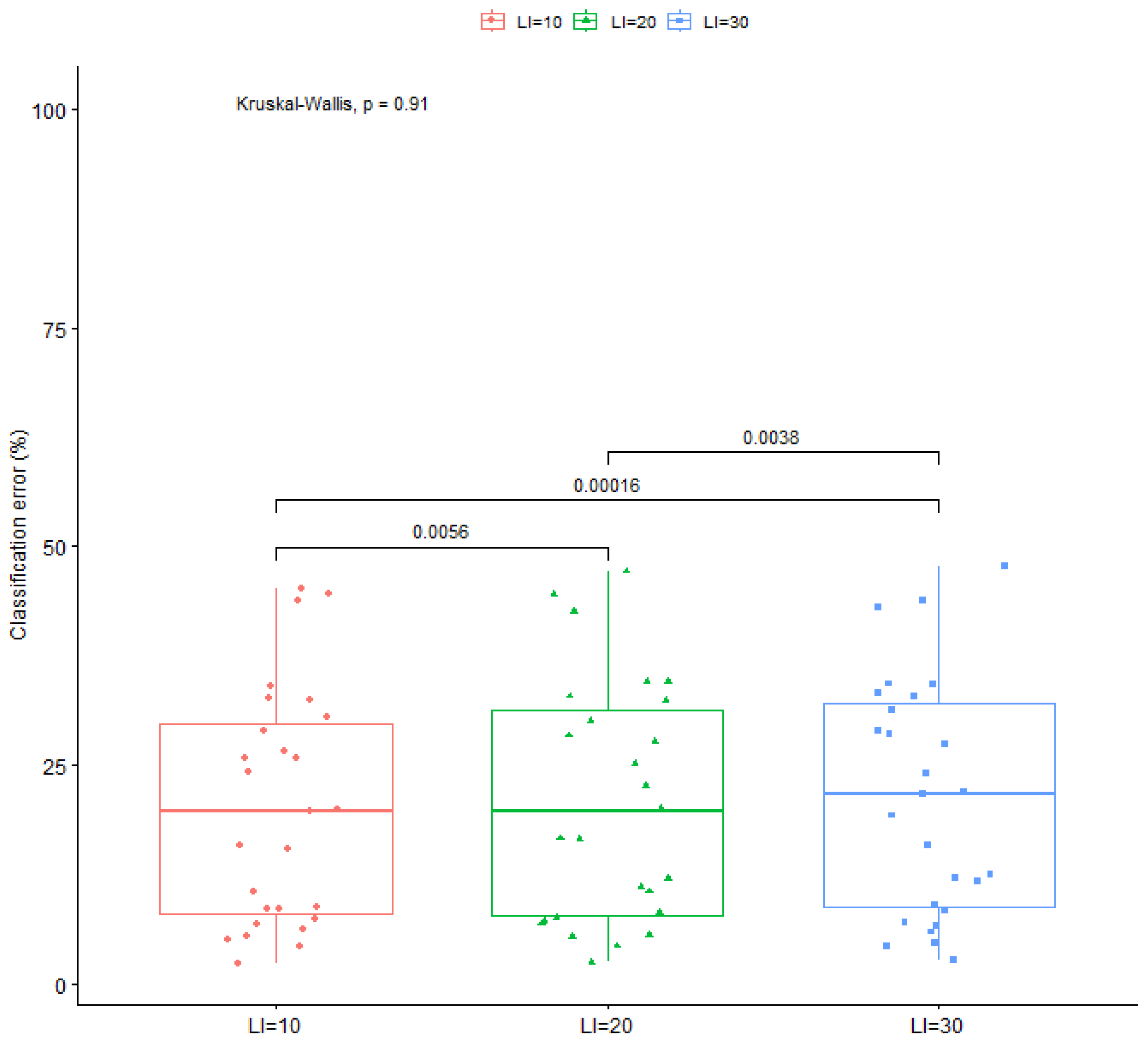
| Dataset | |||
|---|---|---|---|
| APPENDICITIS | 22.30% | 22.60% | 24.20% |
| AUSTRALIAN | 33.78% | 32.42% | 28.72% |
| BALANCE | 8.16% | 8.10% | 8.26% |
| BANDS | 34.81% | 34.53% | 33.97% |
| CIRCULAR | 4.22% | 4.35% | 4.38% |
| CLEVELAND | 46.24% | 42.62% | 44.58% |
| DERMATOLOGY | 16.69% | 12.12% | 9.94% |
| ECOLI | 50.64% | 47.18% | 45.24% |
| FERT | 26.60% | 25.20% | 25.90% |
| HEART | 23.96% | 16.59% | 15.15% |
| HEARTATTACK | 25.70% | 20.13% | 19.97% |
| HOUSEVOTES | 6.74% | 7.13% | 7.44% |
| LIVERDISORDER | 34.50% | 32.88% | 32.50% |
| PARKINSONS | 16.53% | 16.63% | 15.68% |
| PIMA | 33.18% | 30.08% | 26.33% |
| POPFAILURES | 4.52% | 5.44% | 5.89% |
| REGIONS2 | 30.86% | 27.69% | 26.40% |
| SAHEART | 35.68% | 34.56% | 32.67% |
| SEGMENT | 32.53% | 28.41% | 26.15% |
| SONAR | 21.40% | 19.80% | 19.80% |
| SPIRAL | 45.15% | 44.54% | 44.23% |
| WDBC | 7.38% | 5.66% | 4.91% |
| WINE | 16.06% | 10.59% | 8.82% |
| Z_F_S | 18.20% | 11.10% | 8.60% |
| ZO_NF_S | 16.80% | 6.86% | 6.22% |
| ZONF_S | 2.92% | 2.48% | 2.42% |
| ZOO | 7.60% | 7.60% | 6.80% |
| AVERAGE | 23.08% | 20.64% | 19.82% |
| Dataset | |||
|---|---|---|---|
| APPENDICITIS | 23.70% | 22.60% | 22.50% |
| AUSTRALIAN | 32.60% | 32.42% | 31.51% |
| BALANCE | 8.36% | 8.10% | 8.05% |
| BANDS | 34.28% | 34.53% | 33.75% |
| CIRCULAR | 4.48% | 4.35% | 4.51% |
| CLEVELAND | 43.38% | 42.62% | 43.24% |
| DERMATOLOGY | 13.97% | 12.12% | 11.26% |
| ECOLI | 47.79% | 47.18% | 47.06% |
| FERT | 26.50% | 25.20% | 26.70% |
| HEART | 20.67% | 16.59% | 16.18% |
| HEARTATTACK | 23.20% | 20.13% | 20.43% |
| HOUSEVOTES | 7.30% | 7.13% | 7.44% |
| LIVERDISORDER | 32.50% | 32.88% | 33.09% |
| PARKINSONS | 16.63% | 16.63% | 15.26% |
| PIMA | 31.89% | 30.08% | 28.04% |
| POPFAILURES | 4.43% | 5.44% | 5.48% |
| REGIONS2 | 29.71% | 27.69% | 26.99% |
| SAHEART | 34.28% | 34.56% | 33.26% |
| SEGMENT | 29.19% | 28.41% | 27.46% |
| SONAR | 20.95% | 19.80% | 20.05% |
| SPIRAL | 44.17% | 44.54% | 44.20% |
| WDBC | 6.48% | 5.66% | 5.45% |
| WINE | 12.76% | 10.59% | 10.41% |
| Z_F_S | 13.50% | 11.10% | 8.70% |
| ZO_NF_S | 15.14% | 6.86% | 7.28% |
| ZONF_S | 2.44% | 2.48% | 2.38% |
| ZOO | 7.40% | 7.60% | 7.60% |
| AVERAGE | 21.77% | 20.64% | 20.31% |
| Dataset | |||
|---|---|---|---|
| APPENDICITIS | 24.20% | 22.60% | 24.10% |
| AUSTRALIAN | 30.49% | 32.42% | 33.22% |
| BALANCE | 8.50% | 8.10% | 8.44% |
| BANDS | 34.08% | 34.53% | 34.22% |
| CIRCULAR | 4.29% | 4.35% | 4.36% |
| CLEVELAND | 44.58% | 42.62% | 43.10% |
| DERMATOLOGY | 10.63% | 12.12% | 12.54% |
| ECOLI | 45.24% | 47.18% | 47.67% |
| FERT | 25.90% | 25.20% | 27.30% |
| HEART | 15.44% | 16.59% | 19.26% |
| HEARTATTACK | 19.87% | 20.13% | 21.83% |
| HOUSEVOTES | 7.44% | 7.13% | 6.65% |
| LIVERDISORDER | 32.50% | 32.88% | 32.85% |
| PARKINSONS | 15.89% | 16.63% | 15.79% |
| PIMA | 28.96% | 30.08% | 31.28% |
| POPFAILURES | 5.13% | 5.44% | 4.76% |
| REGIONS2 | 25.74% | 27.69% | 28.98% |
| SAHEART | 32.67% | 34.56% | 34.33% |
| SEGMENT | 26.55% | 28.41% | 28.62% |
| SONAR | 19.80% | 19.80% | 21.69% |
| SPIRAL | 43.82% | 44.54% | 43.85% |
| WDBC | 5.48% | 5.66% | 5.95% |
| WINE | 8.82% | 10.59% | 11.65% |
| Z_F_S | 8.60% | 11.10% | 12.13% |
| ZO_NF_S | 6.22% | 6.86% | 9.06% |
| ZONF_S | 2.42% | 2.48% | 2.64% |
| ZOO | 6.80% | 7.60% | 7.10% |
| AVERAGE | 20.00% | 20.64% | 21.24% |
Disclaimer/Publisher’s Note: The statements, opinions and data contained in all publications are solely those of the individual author(s) and contributor(s) and not of MDPI and/or the editor(s). MDPI and/or the editor(s) disclaim responsibility for any injury to people or property resulting from any ideas, methods, instructions or products referred to in the content. |
© 2024 by the authors. Licensee MDPI, Basel, Switzerland. This article is an open access article distributed under the terms and conditions of the Creative Commons Attribution (CC BY) license (https://creativecommons.org/licenses/by/4.0/).
Share and Cite
Tsoulos, I.G.; Charilogis, V.; Tsalikakis, D. Train Neural Networks with a Hybrid Method That Incorporates a Novel Simulated Annealing Procedure. AppliedMath 2024, 4, 1143-1161. https://doi.org/10.3390/appliedmath4030061
Tsoulos IG, Charilogis V, Tsalikakis D. Train Neural Networks with a Hybrid Method That Incorporates a Novel Simulated Annealing Procedure. AppliedMath. 2024; 4(3):1143-1161. https://doi.org/10.3390/appliedmath4030061
Chicago/Turabian StyleTsoulos, Ioannis G., Vasileios Charilogis, and Dimitrios Tsalikakis. 2024. "Train Neural Networks with a Hybrid Method That Incorporates a Novel Simulated Annealing Procedure" AppliedMath 4, no. 3: 1143-1161. https://doi.org/10.3390/appliedmath4030061
APA StyleTsoulos, I. G., Charilogis, V., & Tsalikakis, D. (2024). Train Neural Networks with a Hybrid Method That Incorporates a Novel Simulated Annealing Procedure. AppliedMath, 4(3), 1143-1161. https://doi.org/10.3390/appliedmath4030061