Factorization and Closed Form of Quantum Density Operators and Related Multiplicity

Abstract

The final goal of this paper is to organize the tools needed to study digital Quantum Communications, where classical information is entrusted to quantum states represented by density operators. A density operator is usually defined starting from a set of kets in the Hilbert space and a probability distribution. A fundamental problem in Quantum Communications is the factorization of such operators of the form $\rho =\gamma {\gamma }^{*}$, where $\gamma$ is a matrix called a density factor (DF). The environments considered are finite dimensional Hilbert space (discrete variables) and infinite dimensional Hilbert space (continuous variables). Using discrete variables, the multiplicity and the variety of DFs are investigated using the tools of matrix analysis, arriving in particular to establish the DF with minimal size. With continuous variables, the target is the closed-form factorization, which is achieved with recent results for the important class of Gaussian states. Finally, an application is carried out in Quantum Communications with noisy Gaussian states.

1. Introduction

To introduce the topic of this paper, let us consider the scheme of digital Quantum Communications depicted in Figure 1, where the target is the transmission of classical information, encoded in a sequence symbols $\left\{A_n\right\}$ through quantum states. The transmitter (Alice) reading the symbol $A_n$ sends a quantum state $|{\gamma }_{A_n}\rangle$ through a quantum channel. The receiver (Bob) performs a quantum measurement to guess the received state and then the original symbol. Neglecting noise, the pure state $|{\gamma }_{A_n}\rangle$ is seen by the receiver. In the presence of noise, the received quantum state becomes noisy and must be modeled as a density operator. From this premise, it is clear that the density operator has an absolute leading role in Quantum Communications.

The density operator is usually defined starting from a set of kets in the Hilbert space and a probability distribution. A fundamental problem in Quantum Communications is the factorization of such operators of the form $\rho =\mathit{\gamma }{\mathit{\gamma }}^{*}$, where $\mathit{\gamma }$ is a matrix, called a density factor here, and ${\mathit{\gamma }}^{*}$ is the transpose conjugate of $\mathit{\gamma }$. The environments considered are finite dimensional Hilbert space (discrete variables) and infinite dimensional Hilbert space (continuous variables). Using discrete variables, the multiplicity and the variety of DFs are investigated using the tools of matrix analysis, arriving in particular to establish the DF with minimal size. With continuous variables, the target is the closed-form factorization, which is achieved with recent results for the important class of Gaussian states.

The paper is organized as follows. Only single-mode states are considered. In Section 2, the general definitions of the density operator and density factor are outlined. In the same section, after the definitions, we expose the main tools to proceed, mainly the EID, the SVD, and the FOEX (Fock expansion). Section 3 is dedicated to discrete variables, where the states live in a finite-dimensional Hilbert space ${\mathcal{H}}_n$. Section 4 is dedicated to continuous variables, where the states live in an infinite-dimensional Hilbert space ${\mathcal{H}}_{\infty }$, and the closed form becomes a difficult problem. In Section 5, we introduce Gaussian states, which represent the most important class in the field of continuous variables. We follow the theory of Ma and Rhodes [1,2], who proved that every pure Gaussian state can be generated as a cascade combination of a displacement, a rotation, and a squeezing, and, with the addition of thermal noise, each state also gives mixed Gaussian states. In Section 6 is exposed, in closed form, the Fock expansion of a mixed Gaussian through the “Hermite-like” polynomials. Section 7 introduces two other important tools: the inner product of two quantum states, used in Helstrom bound and in square root measurements, and the mean number of photon in a pure quantum state, which are used in Quantum Communications systems. Finally, in Section 8, an application to digital quantum communications is considered, where the classical information is carried out by Gaussian states.

Remark 1.

“Closed Form” is a critical term for the paper. For example, an infinite sum would generally not be considered a closed form. We give a precise meaning to the notion of a closed form: we intend an algebraic calculation where the complexity is limited to the Galois group of radicals and to the ordinary functions as exponentials, as well as trigonometric and hyperbolic functions.

2. Definitions and Tools

2.1. Definition of Density Operator and Density Factor

Quantum mechanics are formulated in the Hilbert space on the field of complex number. This space may have finite dimensions (discrete variables) or infinite dimensions (continuous variables). We denote the Hilbert space by ${\mathcal{H}}_n$, with k as a natural, $k\ge 1$, in the first case, and ${\mathcal{H}}_{\infty }$ in the second case. Mathematical tools and targets may be very different in ${\mathcal{H}}_n$ and ${\mathcal{H}}_{\infty }$.

A density operator is introduced in the following form:

$$\rho =\sum _{i=1}^k|{\gamma }_i\rangle \langle {\gamma }_i|=\mathit{\gamma }{\mathit{\gamma }}^{*}\mathrm{with}\mathit{\gamma }=\left[|{\gamma }_1\rangle ,\dots ,|{\gamma }_k\rangle \right]$$

(1)

where $|{\gamma }_i\rangle$ are unnormalized quantum states of ${\mathcal{H}}_n$ or of ${\mathcal{H}}_{\infty }$. (Note that $|{\gamma }_i\rangle \in {\mathcal{H}}_m$ are m-length column vectors so that $\mathit{\gamma }$ is an $m\times k$ matrix, where $m=n$ is used for discrete variables and $m=\infty$ is used for continuous variables.).

The properties of a density operator are as follows: $\rho$ is a Hermitian PSD operator with a unitary trace. Moreover, the inner products $p_i:=\langle {\gamma }_i|{\gamma }_i\rangle$ define a probability distribution: ${\left\{p_i\right\}}_{i=1,\dots ,k}$.

The $1\times k$ matrix $\mathit{\gamma }$ may be regarded as a representation of the given density operator $\rho$, since it contains all the information of $\rho$. We will call $\mathit{\gamma }$ a density factor (DF) associated to the given $\rho$.

Note that, while a DF $\mathit{\gamma }$ uniquely determines a density operator $\rho$, for a given $\rho$, one may find infinitely many DFs $\gamma$, also with different lengths k, that give $\rho =\mathit{\gamma }{\mathit{\gamma }}^{*}$. One of our purposes is to investigate the multiplicity of the possible density operators and density factors. Then, we have a direct problem: given a density operator $\rho$, find a density factor $\mathit{\gamma }$ such that $\rho =\mathit{\gamma }{\mathit{\gamma }}^{*}$ (factorization) and we have an inverse problem: given a density factor $\mathit{\gamma }$, find a density operator such that $\rho =\mathit{\gamma }{\mathit{\gamma }}^{*}$. The inverse problem seems to be trivial, but one of our targets is the closed form, which is not trivial with infinite dimensions. The mathematical tools needed depend strongly on the dimension of Hilbert space: in ${\mathcal{H}}_n$, one can use both the EID and the SVD, whereas in ${\mathcal{H}}_{\infty }$, the only tool is the FOEX. To proceed with the theory, we need to recall these tools.

2.2. Eigendecomposition of a Hermitian Matrix

The EID is formulated in different forms. Here, we choose a convenient form for the paper. Let $\mathbf{A}$ be an $n\times n$ Hermitian matrix, and let $\left\{{\lambda }_i\right\},i=1,2,\cdots ,n$ be the distinct eigenvalues of $\mathbf{A}$. Then, the EID of $\mathbf{A}$ results in

$$\mathbf{A}=\sum _{i=1}^n{\lambda }_i|b_i\rangle \langle b_i|=\mathbf{U}\Lambda {\mathbf{U}}^{*},$$

(2)

where $|b_i\rangle ,i=0,1,\dots ,n$ is a orthonormal basis of ${\mathcal{H}}_n$. The rank of $\mathbf{A}$ is given by the number of nonzero eigenvalues ${\tilde{\lambda }}_i$; if $\mathbf{A}$ has the eigenvalue 0 with multiplicity $p_0$, the rank results in $r=n-p_0$. Then, the EID can be written in the following form, which we call a reduced EID:

$$\mathbf{A}=\sum _{i=1}^r{\tilde{\lambda }}_i|b_i\rangle \langle b_i|={\mathbf{U}}_r{\tilde{\Lambda }}_r{\mathbf{U}}_r^{*},$$

(3)

where ${\mathbf{U}}_r=\left[\right|b_1\rangle ,|b_2\rangle ,\dots ,|b_r\rangle ]$ is $n\times r$, and ${\tilde{\Lambda }}_r=\mathrm{diag}[{\tilde{\lambda }}_1,{\tilde{\lambda }}_2,\dots ,{\tilde{\lambda }}_r]$ is $r\times r$.

The EID is often called diagonalization. In this regard, we recall [3], which states that a matrix is uniquely diagonalizable, up to a permutation, if and only if its eigenvalues are all distinct.

2.3. Singular-Value Decomposition (SVD)

So far, we have considered complex square matrices. The SVD considers more generally complex rectangular matrices.

Theorem 1.

The singular-value decomposition of an $m\times n$ matrix $\mathbf{A}$ results in

$$\mathbf{A}=\mathbf{U}\mathbf{D}{\mathbf{V}}^{*},$$

(4)

where $\mathbf{U}$ is an $m\times m$ unitary matrix, $\mathbf{V}$ is an $n\times n$ unitary matrix, and $\mathbf{D}$ is an $m\times n$ diagonal matrix with real non-negative values on the diagonal.

The positive values $d_i$ of the diagonal matrix $\mathbf{D}$ are called the singular values of $\mathbf{A}$. The SVD of a matrix $\mathbf{A}$ is strictly connected to the EIDs of the Hermitian matrices $\mathbf{A}{\mathbf{A}}^{*}$ and ${\mathbf{A}}^{*}\mathbf{A}$ (see [3] and Ch. 2 of [4]).

If the matrix has rank r, the positive values $d_i$ are r, and a more explicit form can be given for the decomposition:

$$\mathbf{A}={\mathbf{U}}_r{\mathbf{D}}_r{\mathbf{V}}_r^{*}=\sum _{i=1}^r{d}_i|u_i\rangle \langle v_i|,$$

(5)

where ${\mathbf{U}}_r=\left[\right|u_1\rangle \cdots |u_r\rangle ]$ is an $m\times r$ matrix, ${\mathbf{V}}_r=\left[\right|v_1\rangle \cdots |v_r\rangle ]$ is an $n\times r$ matrix, and ${\mathbf{D}}_r$ is an $r\times r$ diagonal matrix collecting on the diagonal the singular values $d_i$.

2.4. Fock Expansion (FOEX) and Thermal States

The FOEX is generated by the number operator, which is defined as

$$N=a^{*}a,$$

(6)

where a is the annihilator operator, $a^{*}$ is the creator operator, and clearly N is a Hermitian operator (observable). The corresponding eigenvalue equation is $N|n\rangle =n|n\rangle$, where the eigenkets $|n\rangle$ are called the number states and also the Fock states. The infinite sequence of Fock states $\mathcal{F}:=\left\{\right|n\rangle ,n=0,1,2,\dots \}$ forms an orthonormal basis. The application of this basis to a ket $|\mathbf{x}\rangle$ gives the FOEX of $|\mathbf{x}\rangle$:

$$|\mathbf{x}\rangle =\sum _{n=0}^{\infty }{f}_n|n\rangle \mathrm{with}{f}_n=\langle n|\mathbf{x}\rangle$$

(7)

And the application to a matrix (or to an operator) $\mathbf{A}$ gives the FOCK of $\mathbf{A}$:

$$\mathbf{A}=\sum _{m,n=0}^{\infty }{A}_{mn}\mathrm{with}{A}_{mn}=\langle m\left|\mathbf{A}\right|n\rangle .$$

(8)

The thermal state plays a fundamental role both for the theory of quantum mechanics (thermal states are also defined as the bosonic states that maximize the von Neumann entropy for a fixed energy, as pointed out by Weedbrook et al. [5]) and its applications (see, for instance, Quantum Communications). Glauber [6] obtained the following Fock expansion for the density operator of thermal noise (of a resonant cavity in thermal equilibrium at a absolute temperature $T_0$):

$${\rho }_{\mathrm{th}}={\displaystyle \frac{1}{\mathcal{N}+1}}\sum _{n=0}^{\infty }{\left({\displaystyle \frac{\mathcal{N}}{\mathcal{N}+1}}\right)}^n|n\rangle \langle n|$$

(9)

and the corresponding Fock coefficients

$${\rho }_{mn}={\displaystyle \frac{1}{\mathcal{N}+1}}{\left({\displaystyle \frac{\mathcal{N}}{\mathcal{N}+1}}\right)}^n{\delta }_{mn},$$

(10)

where ${\delta }_{mn}$ is the Kronecker delta, and $\mathcal{N}$ is defined by $\mathcal{N}=1/\left[\exp (h\nu /k{T}_0-1)\right]$ with h being Plank’s constant, k being Boltzmann’s constant, and $\nu$ being the frequency of the specific mode. The interpretation of $\mathcal{N}$ is the average number of thermal photons, which we call here the number of thermal photons.

3. Multiplicity with Discrete Variables

This topic is not new and was considered by several authors. In particular, in 1993, Hugston, Josa, and Wootters in a letter [7] remarked that different probability basis sets may give the same density operator. Later on in 2015, the first author of this paper in the book [4] reconsidered this multiplicity in a new form, completely based on matrix analysis, with application of the SVD and of the EID. In particular, the SVD states a clear link between the EID of a density operator and its density factors. This plays a fundamental role in quantum detection based on the square root measurement (SQRM) and also in several other applications.

Density Factors of a Given Density Operator

A DF $\mathit{\gamma }$ of $\rho$ with k components will be called a k-DF. It is easy to see that the minimum value of k is given by the rank r of $\rho$, which is also the rank of any DF of $\rho$, but the value of k may be arbitrarily large. An r-DF, with $r=\mathrm{rank}\left(\rho \right)$, will be called a minimum density factor of $\rho$. A DF $\left.\mathit{\gamma }=\left[\left|{\mathit{\gamma }}_1\right.〉|,\dots ,|{\mathit{\gamma }}_k\right.〉\right]$, where the states are orthonormal, will be called an orthonormal density factor of $\rho$. Note that an orthonormal k-DF $\mathit{\gamma }$ is necessarily minimum.

In the following proposition, we outline two statements concerning the minimum factor. The proof is essentially based on the orthonormality of the bases (see [4]).

Proposition 1.

Let ρ be a density operator in an n-dimensional Hilbert space $\mathcal{H}$ and let $r=\mathrm{rank}\left(\rho \right)$. Then, we have the following:

(1) 

The minimum density factor of ρ. Consider the reduced EID of ρ:

$$\rho =\sum _{i=1}^r{\sigma }_i^2\left|{\widehat{\mathbf{u}}}_i\right.〉\left.〈{\widehat{\mathbf{u}}}_i\right|=\widehat{\mathbf{U}}{\mathsf{\Sigma }}^2{\widehat{\mathbf{U}}}^{*},$$

(11)

where ${\sigma }_i^2$ are the r positive eigenvalues of $\rho ,\left|{\widehat{\mathbf{u}}}_i\right.〉$ are the corresponding orthonormal eigenvectors, $\widehat{\mathbf{U}}=\left[\left|{\widehat{\mathbf{u}}}_1\right.〉,\dots ,\left|{\widehat{\mathbf{u}}}_r\right.〉\right]$, and ${\mathsf{\Sigma }}^2=\mathrm{diag}\left\{{\sigma }_1^2,\dots ,{\sigma }_r^2\right\}$. Then,

$${\gamma }_0=\widehat{\mathbf{U}}\mathsf{\Sigma }=\left[{\mathbf{u}}_1,\dots ,{\mathbf{u}}_r\right],with{\mathbf{u}}_i={\sigma }_i{\widehat{\mathbf{u}}}_i$$

(12)

is a minimum DF of ρ.

(2) 

Arbitrary DF from a minimum DF. An arbitrary k-DF Φ of ρ is related to a reference minimum orthonormal DF ${\mathit{\gamma }}_0$ in the form $\Phi ={\mathit{\gamma }}_0{A}_0$, where ${\mathbf{A}}_0$ is an $r\times k$ matrix given by

$${\mathbf{A}}_0={\mathsf{\Sigma }}^{-2}{\mathit{\gamma }}_0^{*}\Phi ,$$

(13)

with ${\Sigma }^2$ being the diagonal matrix formed by the positive eigenvalues of ρ. The matrix ${\mathbf{A}}_0$ always verifies the condition ${\mathbf{A}}_0{\mathbf{A}}_0^{*}={\mathbf{I}}_r$, where ${\mathbf{I}}_r$ is the identity matrix of order r.

4. Closed-Form Factorization with Continuous Variables

4.1. State Matrices with Mixed States

We recall that, with pure states, the density operators have the factorized form $\rho =|\mathit{\gamma }\rangle \langle \mathit{\gamma }|$ and, with standard notation, $\rho =\mathit{\gamma }{\mathit{\gamma }}^{*}$, where the states $\mathit{\gamma }=|\mathit{\gamma }\rangle$ are column vectors. In the general case, the density operators is not given as a product of two factors, but it can be factorized in the form

$$\rho =\mathit{\gamma }{\mathit{\gamma }}^{*},$$

(14)

where the $\mathit{\gamma }$s are matrices of appropriate dimensions (and not simply column vectors). In ${\mathcal{H}}_n$, the matrix $\mathit{\gamma }$ can be chosen of dimensions $n\times h$, where h is the rank of $\rho$. But such factorization is not unique, because h has the constraint $\mathrm{rank}\left(\rho \right)\le h\le n$. However, the minimal choice $h=\mathrm{rank}\left(\rho \right)$ is the most convenient (and in the following, we will comply with this choice).

4.2. How to Obtain a Factorization with Continuous Variables

In the previous sections, the factorization of a density operator was developed starting from an ensemble of probabilities/states. Now, consider a generic density operator $\rho$ of dimensions $n\times n$ and rank h. Then, the factorization $\rho =\gamma {\gamma }^{*}$ can be obtained using its reduced EID:

$$\rho ={\mathbf{Z}}_h{\mathbf{D}}_h^2{\mathbf{Z}}_h^{*}=\sum _{i=1}^h{d}_i^2|z_i\rangle \langle z_i|,$$

(15)

where ${\mathbf{D}}_h^2=\mathrm{diag}[d_1^2,\dots ,d_h^2]$ contains in the diagonal h and the positive eigenvalues of $\rho$, and ${\mathbf{Z}}_h=\left[\right|z_1\rangle \cdots |z_h\rangle ]$ is an $n\times h$ matrix. Then, a density factor of $\rho$ is given by

$$\gamma ={\mathbf{Z}}_h{\mathbf{D}}_h=\sum _{i=1}^h{d}_i|z_i\rangle ,$$

(16)

where ${\mathbf{D}}_h=\sqrt{{\mathbf{D}}_h^2}=\mathrm{diag}[d_1,\dots ,d_h]$.

In conclusion, the density operator is decomposed into elementary operators $d_i|z_i\rangle$, where $d_i$ gives the probability that the quantum system is in the state $|z_i\rangle$, as in the original definition of the density operator.

4.3. Factorization of an Infinite-Dimensional Density Operator

In the infinite-dimensional Hilbert space, the EID cannot be applied, whereas the application of Fock expansion is possible. In fact, a generic density operator $\rho$, not necessarily Gaussian, is represented by an infinite-dimensional matrix $\rho =\left[{\rho }_{mn}\right]$, which is obtained with the Fock basis as

$${\rho }_{mn}=\langle m\left|\rho \right|n\rangle ,m,n=0,1,2,\dots .$$

(17)

where

$$\rho =\sum _{m,n=0}^{\infty }|m\rangle {\rho }_{mn}\langle n|.$$

(18)

The problem is that, knowing the expression of $\rho$ in terms of its specification parameters, one has to calculate the elements ${\rho }_{mn}$ from (17), which are infinitely many. If one is able to calculate ${\rho }_{mn}$ in a closed form, the problem is solved, as seen in the theory of thermal noise and, as we will see, for Gaussian states in the next sections.

5. Definition of Gaussian States

Gaussian states represent the most important class in the field of continuous variables. We consider Gaussian states in the single mode, although the formulation holds also for multimode state with appropriated interpretation of the symbols. These states may be defined through the Wigner function $W(x,y)$, which should have a multivariate Gaussian form, and hence, they are completely specified by the mean vector and the covariance matrix. This is in perfect analogy with the classical definition of probability theory for Gaussian random vectors.

Definition 1.

Let ${\rho }_G=|\gamma \rangle \langle \gamma |$ be a quantum state and let

$$\mathbf{m}=\left[\begin{array}{c}\overline{q}\\ \overline{p}\end{array}\right],\mathbf{V}=\left[\begin{array}{cc}{V}_{11}& V_{12}\\ V_{12}& V_{22}\end{array}\right]$$

(19)

be, respectively, its mean vector and its covariance matrix. Then, ${\rho }_G=|\gamma \rangle \langle \gamma |$ is a Gaussian state if its Wigner function results in

$$W(x,y)={\displaystyle \frac{1}{2\pi }}{e}^{-{\displaystyle \frac{1}{2}}\left[V_{22}{(x-\overline{q})}^2+V_{11}{(y-\overline{p})}^2-2V_{12}(x-\overline{q})(y-\overline{p})\right]}$$

(20)

Definition 2.

A unitary operator $U_G$ is called a Gaussian unitary when it transforms Gaussian states into Gaussian states.

We remark that the Wigner function has a multivariate Gaussian form, and hence, Gaussian states are completely specified by the mean vector and the covariance matrix. This is in analogy with the definition of Gaussian random vectors from probability theory. We also remark that the definition of Gaussian unitary is in harmony with the theory of stochastic processes in linear systems, where the Gaussianity is preserved.

5.1. Generation of Gaussian States

A pure Gaussian state is generated starting from the ground state $|0\rangle$, which is itself a Gaussian state, in the form

$${|\gamma \rangle }_G=U_G|0\rangle \to {\rho }_G={|\gamma \rangle }_G{\langle \gamma |}_G,$$

(21)

where $U_G$ is a Gaussian unitary.

A noisy (mixed) Gaussian state is generated starting from a thermal state ${\rho }_{th}\left(\mathcal{N}\right)$, which is itself a Gaussian state, in the form

$${\rho }_G=U_G{\rho }_{th}\left(\mathcal{N}\right)U_G^{*},$$

(22)

where $U_G$ is a Gaussian unitary.

5.2. Gaussian Unitaries from Primitive Gaussian Unitaries

In books and journals, one may find several different forms of definitions of Gaussian unitaries. In this paper, we follow the form introduced by Ma and Rhodes in two seminal papers [1,2]. Ma and Rhodes claimed that there are only three fundamental Gaussian unitaries (FUGs) from which it is possible to generate all Gaussian unitaries. The three FUGs are the following:

• Displacement operator:   $D\left(\alpha \right):=e^{\alpha a^{*}-{\alpha }^{*}a},\alpha \in \mathbb{C}$
• Rotation operator:     $R\left(\varphi \right):=e^{a^{*}\varphi a},\varphi \in \mathbb{R}$
• Squeeze operator:     $Z\left(z\right):=e^{{\displaystyle \frac{1}{2}}\left[(a^{*}z-a{z}^{*})\right]},z\in \mathbb{C}$

where a and $a^{*}$ are the annihilator and the creator operators. Note that when the parameter is zero, the corresponding unitary degenerates to the identity, e.g., $Z\left(0\right)=I_{\mathcal{H}}$.

In [2], Ma and Rhodes proved the following fundamental result:

Theorem 2.

Any Gaussian unitary $U_G$ can be obtained as the combination of the three fundamental Gaussian unitaries $D\left(\alpha \right)$, $Z\left(z\right)$, and $R\left(\varphi \right)$ and cascaded in any arbitrary order, that is,

$$U_G=Z\left(z\right)D\left(\alpha \right)R\left(\varphi \right),U_G=R\left(\varphi \right)D\left(\alpha \right)Z\left(z\right),etc.$$

(23)

The theorem is illustrated in Figure 2, showing the subsets of the fundamental Gaussian unitaries. Note that any other point out of the subsets is obtained as a cascade combination of two or thre FGUs. For instance, $Z\left(z\right)I_{\mathcal{H}}D\left(\alpha \right)=Z\left(z\right)D\left(\alpha \right)$ gives the displacement–squeeze operator.

• Switching rule: In a cascade, it is possible to switch the order of the FGUs by changing the parameters. For instance, $D\left(\alpha \right)Z\left(z\right)=Z\left(z\right)D\left(\beta \right)$, where $\beta =\cosh r\alpha -\sinh r{e}^{i\theta }{\alpha }^{*}$.

5.3. Generation of Pure and Mixed Gaussian States

The application of a Gaussian unitary to the ground state provides a pure Gaussian state:

$$|{\gamma }_G\rangle =D\left(\alpha \right)Z\left(z\right)|0\rangle ,$$

(24)

Note that the phase operator $R\left(\varphi \right)$ is irrelevant (in the single mode), because $R\left(\varphi \right)|0\rangle =|0\rangle$. For instance, $Z\left(z\right)D\left(\alpha \right)R\left(\varphi \right)|0\rangle =Z(z\left)D\right(\alpha \left)\right|0\rangle$.

Any noisy (mixed) Gaussian state can be generated by applying a thermal state to a Gaussiaan unitary

$${\rho }_G=D\left(\alpha \right)Z\left(z\right){\rho }_{\mathrm{th}}\left(\mathcal{N}\right)Z^{*}\left(z\right)D^{*}\left(\alpha \right)$$

(25)

as illustrated in Figure 3.

Remark 2.

In this case, the phase operator is also irrelevant.

6. Fock Expansion of Pure and Mixed Gaussian States

The Fock expansion of mixed Gaussian was evaluated in a closed form by Pierobon et al. in 2015 [8]. This represents a very important result because it gives the possibility to deal with the whole class of Gaussian states, both pure and mixed. Here, it will be presented in the general case, and thence, we will obtain the specific cases of interest.

We have seen that a noisy Gaussian state is represented by a density operator ${\rho }_G$, which depends on the bosonic parameters (DATA) given by

$$z=r_0{e}^{i\theta }\in \mathbb{C},\alpha \in \mathbb{C},\mathcal{N}\ge 0$$

(26)

where $z=r_0{e}^{i\theta }$ is the squeeze parameter, $\alpha$ is the displacement parameter, and $\mathcal{N}$ gives the average number of photon present in the thermal state. In the bosonic space, ${\rho }_G$ is represented by an infinite dimensional matrix $\rho =\left[{\rho }_{mn}\right]$, which is obtained with the Fock basis as ${\rho }_{mn}=\langle m\left|\rho \right|n\rangle ,m,n=0,1,2,\dots$.

The closed form is based on two powerful Hermite-like polynomials [9]. The first are the two variable versions of the Hermite polynomials

$${\mathcal{H}}_n(x,y)=n!\sum _{r=0}^{\lfloor n/2\rfloor }{\displaystyle \frac{1}{(n-2r)!r!}}{x}^{n-2r}{y}^r,$$

(27)

which are referred as Hermite–Kampé de Feriét polynomials (also called heat polynomials). The second are two-index Hermite–Kampé de Feriét polynomials

$${\mathcal{H}}_{m,n}(x,y;z,u|\tau )=m!n!\sum _{r=0}^{\min [m,n]}{\displaystyle \frac{{\mathcal{H}}_{m-r}(x,y){\mathcal{H}}_{n-r}(z,u){\tau }^r}{(m-r)!r!(n-r)!}}.$$

(28)

The polynomial ${\mathcal{H}}_n(x,y)$ is illustrated in the Figure 4.

The parameters of ${\rho }_{mn}$, which are obtained from the DATA, are the following:

$$\begin{array}{ccccc}& S=\mathrm{sech}\left(r_0\right)\hfill & \hfill T=\tanh \left(r_0\right)e^{i\theta }& x=\alpha S\hfill & \hfill y={\displaystyle \frac{1}{2}}T\\ & Y={\displaystyle \frac{\mathcal{N}}{\mathcal{N}+1}}\hfill & \hfill L={\displaystyle \frac{1}{1-4Y^2{\left|T\right|}^2}}& a=-{\displaystyle \frac{1}{2}}TL{Y}^2\hfill & \hfill b=LY\end{array}$$

(29)

Then, in [8], the following is proved:

Proposition 2.

The Fock coefficients of the general Gaussian state ${\rho }_G$ are given by

$${\rho }_{mn}=J\sum _{r=0}^m\sum _{s=0}^n{K}_{m,r}{W}_{r,s}^{*}{K}_{n,s}^{*},$$

(30)

where

$$\begin{array}{cc}& K_0=S^{1/2}\exp \left\{-{\displaystyle \frac{1}{2}}{\left|\alpha \right|}^2+{\displaystyle \frac{1}{2}}{\alpha }^2{T}^{*}\right\}\hfill \\ & J=(1-Y)L|K_0{|}^2\exp \left\{a{z}^2+a^{*}{\left(z^{*}\right)}^2+bz{z}^{*}\right\}\hfill \\ & K_{m,r}=\sqrt{m!}{\displaystyle \frac{{\mathcal{H}}_{m-r}(x,y)S^r}{(m-r)!r!}},m,r=0,1,2,\dots \hfill \\ & W_{r,s}={\mathcal{H}}_{r,s}(2az+b{z}^{*},a;2a^{*}{z}^{*}+bz,a^{*}|b),r,s=0,1,2,\dots \hfill \end{array}$$

(31)

The corresponding infinite-dimensional matrix reads $\rho =J\mathbf{K}\mathbf{W}{\mathbf{K}}^{*}$, where the matrices $\mathbf{K}=\left[K_{m,r}\right]$ and $\mathbf{W}=\left[W_{r,s}\right]$ are defined by (31); $\mathbf{K}$ is a lower triangular because ${\mathcal{H}}_{m-r}(x,y)=0$ for $r>m$, and $\mathbf{W}$ is Hermitian and positive semidefinite.

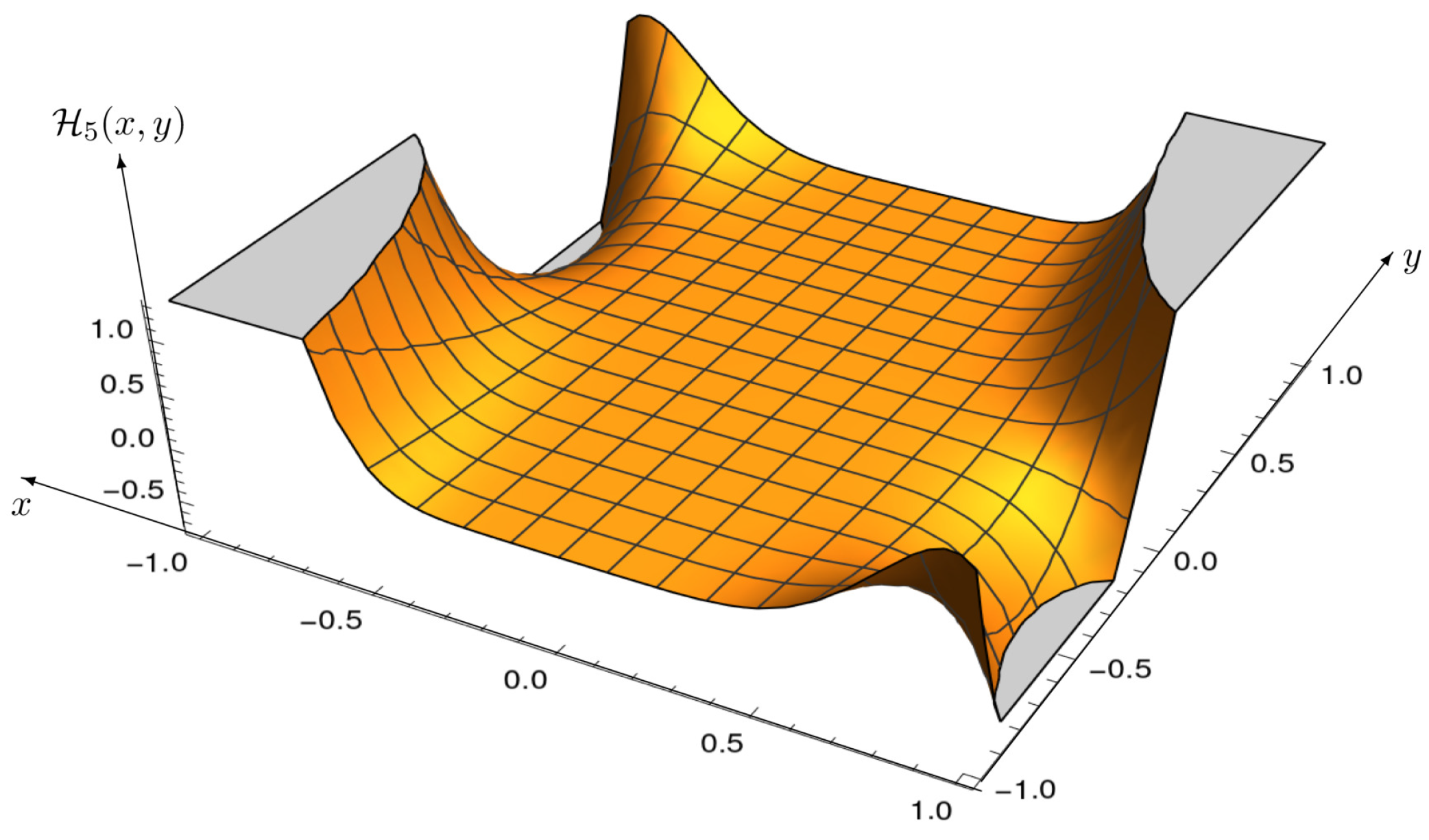
6.1. Fock Expansion of Specific Gaussian States

Proposition 2 holds for a general noisy Gaussian state. It can be particularized to specific cases by setting one or two parameters to zero and by taking into account the following degenerate forms of the Hermite–Kampé de Feriéte polynomials:

$${\mathcal{H}}_n(x,0)=x^n,{\mathcal{H}}_n(0,y)=\left\{\begin{array}{cc}{\displaystyle \frac{y^{n/2}n!}{(n/2)!}}\hfill & \mathrm{for}\mathrm{n}\mathrm{even}\hfill \\ 0\hfill & \mathrm{for}\mathrm{nodd}\hfill \end{array}\right.$$

(32)

Noisy displaced states ($z=0$):

$${\rho }_{mn}={\displaystyle \frac{1}{\mathcal{N}+1}}{\exp (-|\alpha |}^2)\sum _{r=0}^m\sum _{s=0}^n{K}_{mr}\left(\alpha \right)K_{ns}\left({\alpha }^{*}\right)\sum _{j=0}^{\min (r,s)}{P}_{rs|j}\left({\displaystyle \frac{\mathcal{N}}{\mathcal{N}+1}}\right),$$

(33)

where

$$K_{mr}\left(\alpha \right):={\displaystyle \frac{\sqrt{m!}}{(m-r)!r!}}{\alpha }^{m-r},P_{rs|j}\left(Y\right):={\displaystyle \frac{r!}{(r-j)!}}{\displaystyle \frac{s!}{(s-j)!}}{Y}^j.$$

(34)

To prove Equation (33), one needs to use the second of (32) and the expression of the degenerated form:

$${\mathcal{H}}_{rs}(0,0;0,0|Y)=\sum _{j=0}^{\min (r,s)}{\displaystyle \frac{r!}{(r-j)!}}{\displaystyle \frac{s!}{(s-j)!}}{Y}^j=\sum _{j=0}^{\min (r,s)}{P}_{rs|j}\left(Y\right).$$

(35)

In the literature, one finds an alternative formula due to Yuen [10] in terms of the generalized Laguerre polynomial $L_m^{(m-n)}\left(x\right)$.

• Noisy squeezed states ($\alpha =0$): There are not relevant simplifications with respect to the general case apart the use of the second form of Equation (32). Note that in Digital Quantum Communications, the use of this quantum states has no interest because the optical power comes from the displacement.
• Pure Gaussian states ($\mathcal{N}=0$): The Fock coefficients of pure Gaussian states are given by

  $${|z,\alpha \rangle }_n=K_0{\displaystyle \frac{1}{\sqrt{m!}}}{\mathcal{H}}_m(\alpha S,{\displaystyle \frac{1}{2}}T),$$

  (36)

  where $K_0$ is defined in (31). In the literature, the Fock expansion is given by the so-called Yuen’s formula through the ordinary Hermite polynomial [10].
• Pure displaced states ($z=0,\mathcal{N}=0$):

  $${|\alpha \rangle }_n=e^{-{\displaystyle \frac{1}{2}}{\left|\alpha \right|}^2}{\displaystyle \frac{{\alpha }^n}{\sqrt{n}}}$$

  (37)
• Pure squeezed states ($\alpha =0,\mathcal{N}=0$):

  $${|z\rangle }_m=S{\displaystyle \frac{1}{\sqrt{m!}}}{\mathcal{H}}_m(0,{\displaystyle \frac{1}{2}}T)),$$

  (38)

  where $\mathcal{H}(0,y)$ is given by the second of (32) and explicitly by

  $${|z\rangle }_{2m}={\displaystyle \frac{\sqrt{m!}}{2^m(2m!)}}\mathrm{sech}\left(r_0\right){tanh}^m\left(r_0{e}^{i\theta }\right),{|z\rangle }_{2m+1}=0.$$

  (39)

6.2. Other Important Parameters for Quantum Communications

The statistic on photon number n in a pure quantum states and the inner product $\langle {\gamma }_1|{\gamma }_0\rangle$ of two pure quantum states play an important role in Quantum Communications, specifically in the Helstrom bound and in SRM. All these parameters were evaluated in the closed form for Gaussian states by Yuen in his seminal paper of 1975 [11]. The distribution of photon number n, $p_n\left(k\right)=Pr[n=k]$ is simply given by

$$p_n\left(k\right)={\left|\right|z,\alpha \rangle }_k{|}^2,$$

(40)

where ${|z,\alpha \rangle }_k$ are the Fock coefficients evaluated in the previous section. In the absence of squeezing, $p_n\left(k\right)$ becomes a Poisson distribution, but in the presence of squeezing, it becomes quickly far from such a shape. The mean photon number results in

$${\overline{n}}_{|z,\alpha \rangle }={\left|\alpha \right|}^2+{\sinh }^{2}r.$$

(41)

The inner product of two pure Gaussian states results in

$$\langle z_1,{\alpha }_1|z_0,{\alpha }_0\rangle =A^{-{\displaystyle \frac{1}{2}}}\exp \left[-{\displaystyle \frac{A\left(|{\beta }_1{|}^2+{\left|{\beta }_0\right|}^2\right)-2{\beta }_1{\beta }_0^{*}+B{\beta }_1^{*2}-B^{*}{\beta }_0^2}{2A}}\right],$$

(42)

where $z_k=r_k{e}^{i{\theta }_k},{\mu }_k=\cosh \left(r_k\right),{\nu }_k=\sinh \left(r_k\right)e^{i{\theta }_k}$, ${\beta }_k={\mu }_k{\alpha }_k-{\nu }_k{\alpha }_k^{*}$, $A={\mu }_0{\mu }_1^{*}-{\nu }_0{\nu }_1^{*},B={\nu }_0{\mu }_1-{\mu }_0{\nu }_1$.

7. Application: Digital Data Quantum Communications Systems with Gaussian States

We follow the Quantum Communications system considered in the introduction (Figure 1), where the target is the transmission of classical information through quantum states. At the receiver, Bob tries to guess the state using a quantum measurement. The global performance of the system is given by the transition probabilities, that is, the probability that the received symbol is $\widetilde{A_n}=j$ when the transmitted symbol is $A_n=i$. These probabilities are given by

$$p\left(j\right|i)=\mathrm{Tr}\left({\rho }_i{Q}_j\right),i,j\in \mathcal{A},$$

(43)

where $Q_j,j\in \mathcal{A}$ are the quantum measurement operators. Particular interest is given by the correct decision probability $P_c$, which is obtained as

$$P_c={\displaystyle \frac{1}{m}}\sum _{i=0}^{m-1}p\left(i\right|i)={\displaystyle \frac{1}{m}}\sum _{i=0}^{m-1}\mathrm{Tr}\left({\rho }_i{Q}_i\right)$$

(44)

or by the error probability $P_e=1-P_c$. The main problem of quantum detection is finding the measurement which optimizes the detection, according to some predefined fidelity criterion, usually the minimum error probability. Necessary and sufficient conditions for the optimal measurement set have been found in pioneering papers by Helstrom et al. [12], Holevo [13], and by Yuen et al. [11].

7.1. Numerical Problems with Noisy Gaussian States

The main target is the evaluation of the error probability $P_e$. With pure Gaussian states, this evaluation does not exhibit numerical problems because it is based on the inner product, which is known in the closed form. With noisy Gaussian states, the evaluation is based on the Fock representation, which also is known in the closed form, but $\rho$ has an infinite matrix representation, and for the eigendecomposition (EID) needed to find the measurement operators, one has to approximate each $\rho$ of the constellation with a finite square matrix.

$${\rho }_N=\sum _{r=0}^{N-1}\sum _{s=0}^{N-1}{\rho }_{m,n}|m\rangle \langle n|.$$

(45)

Considering that $\rho$ is PSD, Hermitian, and that these properties also hold for its approximation ${\rho }_N$, the EID is expressed in the following forms:

$${\rho }_N={\mathbf{U}}_N{\Lambda }_{\rho }{\mathbf{U}}_N^{*},$$

(46)

where ${\mathbf{U}}_N$ is an $N\times N$ unitary matrix, and ${\Lambda }_{\rho }$ is an $N\times N$ diagonal matrix whose diagonal elements are the (positive) eigenvalues of ${\rho }_N)$.

A useful approximation of $\rho$ is obtained by the trace criterion [4], which is based on the fact that a density operator has a unitary trace, that is,

$$\mathrm{Tr}\left(\rho \right)=\sum _{k=0}^{\infty }{\rho }_{kk}=1.$$

(47)

Then one gets a good approximation if

$$\mathrm{Tr}\left({\rho }_N\right)=\sum _{k=0}^{N_{ϵ}-1}{\rho }_{kk}=\ge 1-ϵ.$$

(48)

where $ϵ$ is the accuracy, and $N=N_{ϵ}$ is the corresponding number of terms. Of course, the accuracy is chosen in dependence on the range of error probability that we want to evaluate.

The Fock representation ${\rho }_{mn}$ and the error probability depend on the DATA:

$$r_0,\theta ,\alpha ,\mathcal{N}.$$

(49)

The target may be the evaluation of the error probability $P_e$ down to $P_e={10}^{-12}$ and reasonable ranges of the parameters may be

$$r_{0}0÷1,\alpha 0÷4,\mathcal{N}0÷0.6,\max (m,n)=100÷150.$$

(50)

A rule of thumb in the choice of the accuracy may be $ϵ={\displaystyle \frac{1}{10}}{P}_e$.

7.2. State and Measurement Matrix, Gram Operator, and Optimal Quantum Decision

In a K-ary Quantum Communications system, the players are given by a constellation of density operators $\{{\rho }_i,i=1,\dots ,K\}$. As we have seen, each ${\rho }_i$ can be factored as ${\rho }_i={\mathit{\gamma }}_i{\mathit{\gamma }}_i^{*}$, where the state factors ${\mathit{\gamma }}_i$ are $n\times h$ matrices. These states factors ${\mathit{\gamma }}_i$ form the state matrix $\mathit{\gamma }=[{\mathit{\gamma }}_0,{\mathit{\gamma }}_1,\dots ,{\mathit{\gamma }}_{K-1}$]. The measurement operators $Q_i={\mathit{\mu }}_i{\mathit{\mu }}_i^{*}$ have the same factorized form of $n\times h$ matrices. Their collection forms the measurement matrix $\mathbf{M}=[{\mathit{\mu }}_0,{\mathit{\mu }}_1,\dots ,{\mathit{\mu }}_{K-1}].$ Moreover, we define the Gram operator as (this is a matrix, but it is called inappropriately as an operator to distinguish it from the Gram’s matrix $\mathbf{G}={\mathit{\gamma }}^{*}\mathit{\gamma }$) $\mathbf{T}=\mathit{\gamma }{\mathit{\gamma }}^{*}$.

The Optimal Quantum Decision is the following: the data are the a priori probabilities of the states. The measurement operators are unknowns, and the usual decision criterion is given by maximization of the correct decision probability $P_e$. Recalling that the correct decision probability is given by (58), and the optimal measurement operators $Q_i$ must be determined from

$$\underset{\left\{Q_i\right\}}{\max }\sum _{i=0}^{K-1}{q}_i\mathrm{Tr}\left({\rho }_i{Q}_i\right).$$

(51)

This evaluation in the closed form is possible only in a few cases, e.g., in the binary case, but not in general. So, we consider the square root measurement (SRM) method, which gives a good suboptimal decision. The SRM is typically used for decision with pure states, but recently in [14], this method was extended to mixed states, allowing for the evaluation of the performance of Digital Quantum Communications systems even in the presence of thermal noise.

Proposition 3.

In the SRM, procedure the optimal measurement matrix is given by (see [4,14])

$${\mathbf{M}}_0={\mathbf{T}}^{-1/2}\Gamma ,$$

(52)

where $\mathbf{T}=\mathit{\gamma }{\mathit{\gamma }}^{*}$ is the Gram operator.

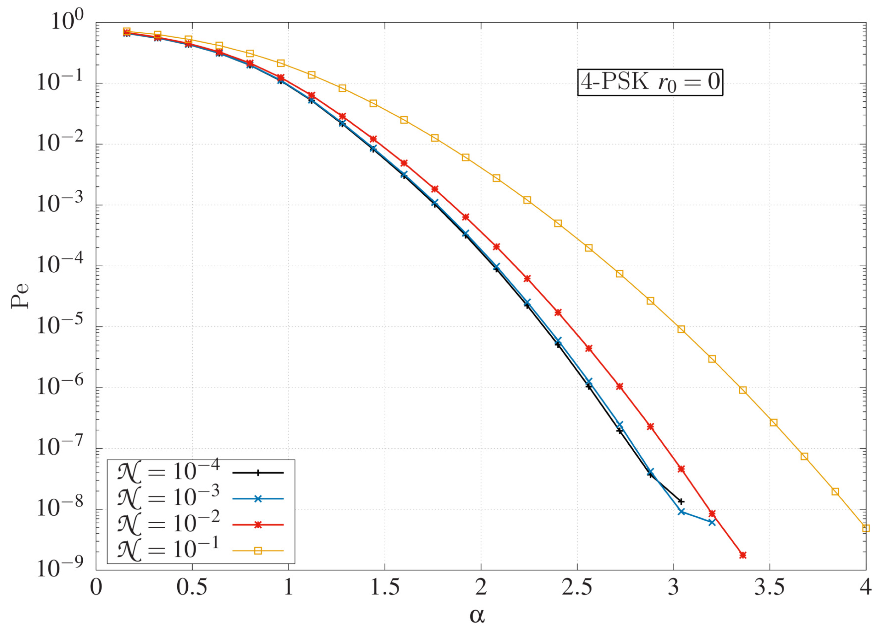
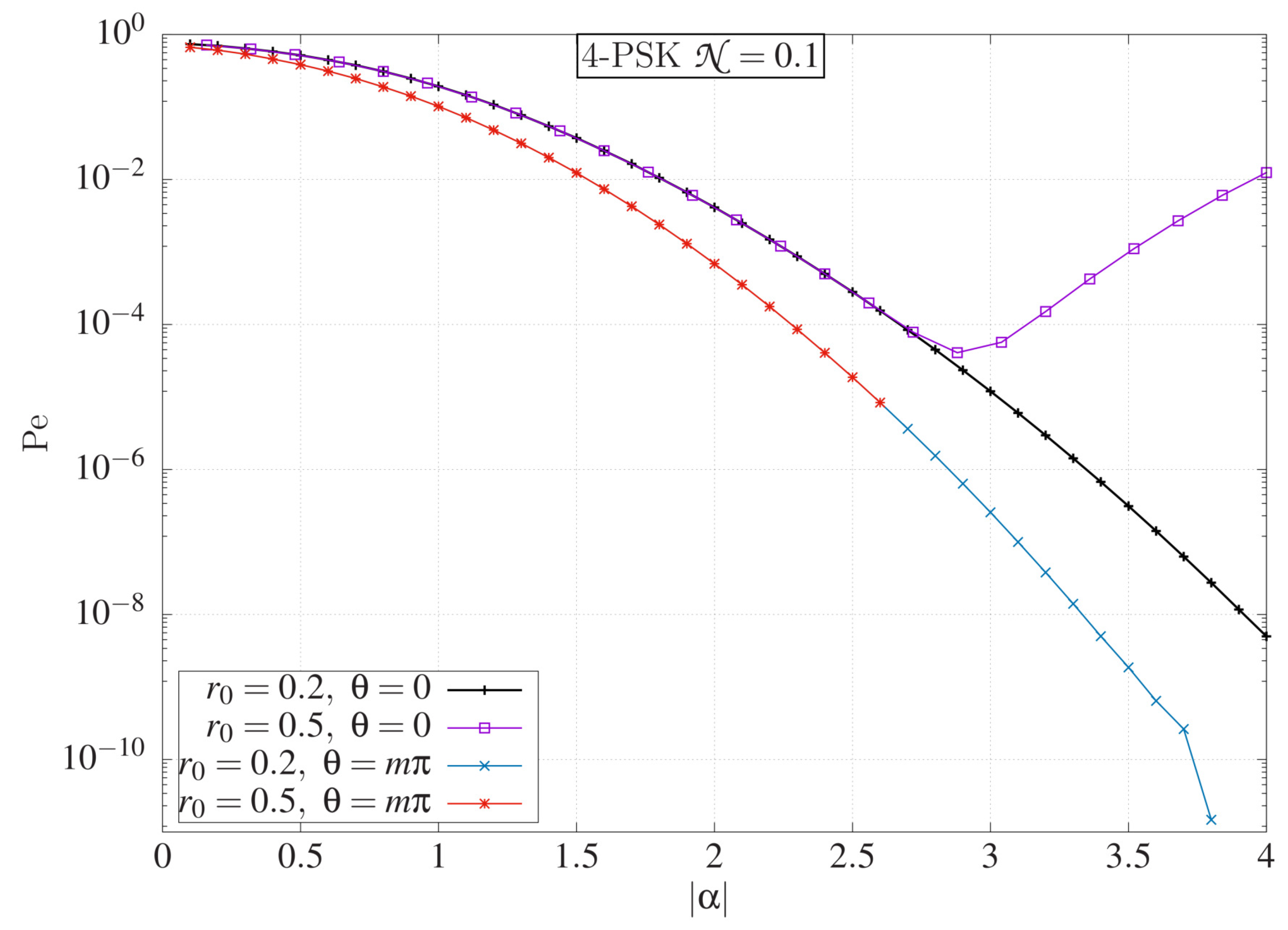
7.3. PSK Quantum Communications Systems in the Presence of Thermal Noise

As a specific example of application, we consider a PSK (phase shift keying) quantum system in the presence of thermal noise, where the constellation of K states is obtained by the reference state ${\rho }_0$ as

$${\rho }_i=S^i{\rho }_0{\left(S^i\right)}^{*},i=0,1,\dots ,K-1.$$

(53)

This extension entails, for the factors, the relation

$${\mathit{\gamma }}_i=S^i{\mathit{\gamma }}_0,i=0,1,\dots ,K-1$$

(54)

and the same symmetry is transferred to the measurement operators

$$Q_i=S^i{Q}_0{\left(S^i\right)}^{*},i=0,1,\dots ,K-1$$

(55)

and to the measurement factors

$${\mathit{\mu }}_i=S^i{\mathit{\mu }}_0,i=0,1,\dots ,K-1.$$

(56)

This constellation satisfies the geometrically uniform symmetry (GUS) with symmetry operator

$$S=\exp \left({\displaystyle \frac{i2\pi }{K}}\mathbf{N}\right)$$

(57)

where $\mathbf{N}$ is the number operator. The SRM theory in the presence of GUS is simplified so much. In fact (see Ch. 6 of [4]), the reference measurement operator is given by

$${\mathbf{Q}}_0={\mathbf{T}}^{-1/2}{\rho }_0{\mathbf{T}}^{-1/2}$$

(58)

Proposition 4.

The transition probabilities with mixed states having the GUS can be obtained from the reference density operator as

$$p_c\left(j\right|i)=\mathrm{Tr}\left[S^{i-j}{\rho }_0{S}^{-(i-j)}{\mathbf{Q}}_0\right]$$

(59)

with ${\mathbf{Q}}_0$ given by (58). The correct decision probability is given by the synthetic formula

$$P_c=\mathrm{Tr}\left[{\rho }_0{(\mathbf{T}}^{-1/2}{)}^2\right].$$

(60)

Two Specific Examples

Using the above theory, we have evaluated the error probability $P_e$ in the general case of Gaussian states in the presence of thermal noise.

In Figure 5, the error probability $P_e$ is plotted versus the displacement parameter $\alpha$ for four values of the number of thermal $\mathcal{N}$ in the absence of squeezing ($z=0$).

In Figure 6, the error probability $P_e$ is plotted versus the displacement parameter $\left|\alpha \right|$ for $\mathcal{N}=0.1$ and four values of the squeezing parameter $z=r_0{e}^{i\theta }$.

8. Conclusions

In the first part of the paper, we have investigated the multiplicity of density factors (DFs) of a given density operator of a finite order. The main result is given by item 2 of Proposition 1, which states that, starting from a minimum orthonormal DF ${\mathit{\gamma }}_0$ of dimension $n\times r$, one can generate all the possible DFs of a given density operator in the form $\mathit{\gamma }={\mathit{\gamma }}_0{\mathbf{A}}_0$, where ${\mathbf{A}}_0$ is an arbitrary $k\times r$ matrix with orthonormal rows, that is, with ${\mathbf{A}}_0{\mathbf{A}}_0^{*}={\mathbf{I}}_r$.

We have seen that the factorization with continuous variables, where the environment is a infinite-dimensional Hilbert space, becomes more difficult, and it may be necessary to proceed with approximations. But, for the important class of Gaussian states, the closed form approximation is possible by virtue of “magic” Hermite-like polynomials. This opportunity can also be achieved for some form of non-Gaussian states, as, e.g., the photon-added displacement states, introduced by Agarwal and Tara in 1991 [15] and recently applied by Guerrini et al. [16] for quantum discrimination in the presence of noise. A group at Padova University is developing a systematic investigation on the performance outcomes of data from Quantum Communications using the closed-form results of Proposition 2 of this paper.

The authors hope to have achieved the ultimate goal of the paper: to provide the mathematical tools and references to investigate new possible Quantum Communications systems, especially based on non-Gaussian states (see in particular the paper [17]). A possible area of application could be deep space Quantum Optical Communications.

References

1. Ma, X.; Rhodes, W. Squeezing in harmonic oscillator with time–dependent frequency. Phys. Rev. A 1989, 39, 1941–1947. [Google Scholar] [CrossRef] [PubMed]
2. Ma, X.; Rhodes, W. Multimode squeeze operators and squeezed states. Phys. Rev. A 1990, 41, 4625–4631. [Google Scholar] [CrossRef] [PubMed]
3. Horn, R.A.; Johnson, C.R. Matrix Analysis; Cambridge University Press: Cambridge, UK, 1998. [Google Scholar]
4. Cariolaro, G. Quantum Communications; Springer: Berlin/Heidelberg, Germany, 2015. [Google Scholar]
5. Weedbrook, C.; Pirandola, S.; García Patrón, R.; Cerf, N.J.; Ralph, T.C.; Shapiro, J.H.; Lloyd, S. Gaussian quantum information. Rev. Mod. Phys. 2012, 84, 621–669. [Google Scholar] [CrossRef]
6. Glauber, R.J. Quantum Theory of Optical Coherence: Selected Papers and Lectures; Wiley-VCH: Hoboken, NJ, USA, 2006. [Google Scholar]
7. Hugston, L.P.; Josa, R.; Wooters, W.K. A complete classification of quantum ensembles having a given density matrix. Phys. Lett. A 1993, 183, 14–18. [Google Scholar] [CrossRef]
8. Pierobon, G.; Cariolaro, G.; Dattoli, G. Fock, Expansion of multimode pure Gaussian states. J. Math. Phys. 2015, 56, 122109. [Google Scholar]
9. Dattoli, G. Incomplete 2D Hermite polynomials: Properties and applications. J. Math. Anal. Appl. 2003, 284, 447–453. [Google Scholar] [CrossRef]
10. Yuen, H.P. Two-photon coherent states of the radiation field. Phys. Rev. A 1976, 13, 2226–2243. [Google Scholar] [CrossRef]
11. Yuen, H.P.; Kennedy, R.; Lax, M. Optimum testing of multiple hypotheses in quantum detection theory. IEEE Trans. Inf. Theory 1975, 21, 125–134. [Google Scholar] [CrossRef]
12. Helstrom, C.W.; Liu, J.W.S.; Gordon, J.P. Quantum–mechanical communication theory. Proc. IEEE 1970, 10, 1578–1598. [Google Scholar] [CrossRef]
13. Holevo, A.S. Statistical decision theory for quantum systems. J. Multivar. Anal. 1973, 3, 337–394. [Google Scholar] [CrossRef]
14. Eldar, Y.C.; Megretski, A.; Verghese, G.C. Optimal detection of symmetric mixed quantum states. IEEE Trans. Inform. Theory 2004, 50, 1198–1207. [Google Scholar] [CrossRef]
15. Agarwal, G.S.; Tara, K. Nonclassical properties of states generated by the excitations on a coherent state. Phys. Rev. A 1991, 43, 492. [Google Scholar] [CrossRef] [PubMed]
16. Guerrini, S.; Win Moe, Z.; Chiani, M.; Conti, A. Quantum Discrimination of Noisy Photon–Added Coherent States. IEEE J. Sel. Areas Inf. Theory 2020, 1, 469–479. [Google Scholar] [CrossRef]
17. Walschaers, M. Non–Gaussian quamtum states and where to find them. PRX Quantum 2021, 2, 030204. [Google Scholar] [CrossRef]
Figure 1. Quantum Communications system for digital transmission. { A n } is a sequence of classical symbols of information that Alice conveys into a sequence of quantum states { | γ A n } . Bob performs a quantum measurement to argue, from the result m of the measurement, which symbol was transmitted.
Appliedmath 05 00013 g001
Figure 2. Gaussian unitaries (operators) and the subclasses of displacement, rotation, and squeezing.
Appliedmath 05 00013 g002
Figure 3. Generation of a noised Gaussian state from the thermal state.
Appliedmath 05 00013 g003
Figure 4. The Hermite–Kampé de Feriét polynomial H n ( x , y ) for n = 5 .
Appliedmath 05 00013 g004
Figure 5. Error probability as a function of α with different values of the number of thermal photons N in the absence of squeezing.
Appliedmath 05 00013 g005
Figure 6. Error probability as a function of | α | with N = 0.1 and different squeezing factors.
Appliedmath 05 00013 g006
Disclaimer/Publisher’s Note: The statements, opinions and data contained in all publications are solely those of the individual author(s) and contributor(s) and not of MDPI and/or the editor(s). MDPI and/or the editor(s) disclaim responsibility for any injury to people or property resulting from any ideas, methods, instructions or products referred to in the content.