Abstract
The modeling of the one-dimensional wave equation is the fundamental model for characterizing the behavior of vibrating strings in different physical systems. In this work, we investigate numerical solutions for the one-dimensional wave equation employing both explicit and implicit finite difference schemes. To evaluate the correctness of our numerical schemes, we perform extensive error analysis looking at the norm of error and relative error. We conduct thorough convergence tests as we refine the discretization resolutions to ensure that the solutions converge in the correct order of accuracy to the exact analytical solution. Using the von Neumann approach, the stability of the numerical schemes are carefully investigated so that both explicit and implicit schemes maintain the stability criteria over simulations. We test the accuracy of our numerical schemes and present a few examples. We compare the solution with the well-known spectral and finite element method. We also show theoretical proof of the stability and convergence of our numerical scheme.
1. Introduction
Wave motion is typically the result of a wide range of physical processes in which signals are transmitted through a medium in space and time, with little or no persistent movement of the medium itself [1,2]. Sepahvand, Marburg, and Hardtke (2007) claim that the numerical approach solves the one-dimensional wave equation with stochastic parameters by combining extended polyp chaos with the finite difference method [2]. Showing great accuracy and efficiency in many numerical examples, Gu, Young, and Fan (2009) present that the method of fundamental solutions (MFS) combined with the Eulerian–Lagrangian method offers a meshless and quadrature-free numerical approach for solving one-dimensional wave equations [3].
Wazwaz (2010) claims that the one-dimensional wave equation defines several physical events including electric signal transmissions, water waves, string vibrations, and electromagnetic and sound wave propagation [4]. In 2006, Nicaise and Pignotti investigated the wave equation with velocity and delay terms inside boundary conditions. Using energy considerations and observability inequalities, they built the conditions for exponential stability [5].
Gao and Ralescu claim that by including stochastic processes like the Wiener and Liu processes to account for random and uncertain sounds, respectively, the uncertain wave equation extends previous deterministic models by a commensurate extent [6]. Investigating the dynamics of a one-dimensional structure without flexural rigidity, Leckar, Sampaio, and Cataldo particularly pay attention to a very light string with vertical motion at every particle [7]. Alabdali and Bakodah (2014) provide a new variation of the method of lines specifically for first-order hyperbolic partial differential equations [8]. On the topic of the numerical solution of partial differential equations, Smith describes in detail the conventional finite difference techniques applied for parabolic, hyperbolic, and elliptic equations [9]. Azam, Pandit, and Andallah (2014) look at a second-order fluid dynamical model utilizing analytical methods and numerical simulations. For the exact numerical solutions, they apply explicit central difference methods, proving convergence rates and error predictions and highlighting the dependability of their method [10].
Md. Shajib Ali, L. S. and Mursheda Begum (2018) produce reliable and efficient numerical solutions for the nonlinear first-order hyperbolic partial differential equations using a second-order Lax–Wendroff finite difference technique [11]. Kreiss, Petersson, and Yström’s (1997) work on strong and accurate numerical techniques for both one- and two-dimensional examples helps to better appreciate difference approximations for the second-order wave equation by specifically demonstrating its application to the complex vibrations of a piano string [12]. Chabessier and Joly (2010) develop a generic energy-preserving methodology for nonlinear Hamiltonian wave systems, therefore stressing the stability and correctness of the given method [13]. By means of analytical and numerical methodologies to solve the vibration string equation, including a fractional derivative, Aleroev and Elsayed (2020) demonstrate the efficacy of the Laplace transform and homotopy perturbation methods in finding solutions defined by Mittag–Leffler functions [14].
Chen and Ding (2008) analyze two nonlinear models for the transverse vibration of strings using numerical solutions to show that, for greater amplitude vibrations, the Kirchhoff equation produces more accurate results; both models perform satisfactorily for low amplitudes [15]. Cumber (2024) shows the application of the method of lines to mimic vibrating strings for instruments like the guitar, piano, and violin, thereby highlighting its simplicity over analytical solutions and its adaptation to advanced models with energy dissipation and stiffness [16]. Starting from linear systems to advance nonlinear mechanisms like hammer–string and bow–string interactions, Bilbao and Ducceschi (2023) present a complete study of string vibration models incorporating collision occurrences [17]. Motivated by earlier research on energy distribution in nonlinear systems, Zabusky (1962) provides a precise solution for the nonlinear vibrations of a continuous string model [18]. Ducceschi and Bilbao (2016) analyze three models of string vibrations in musical acoustics: the Timoshenko model, the traditional Euler–Bernoulli beam equation, and a shear beam equation model. This work evaluates the accuracy of these models in defining string dynamics and their perceptual repercussions for musical acoustics, therefore underlining the restrictions in the conventional approach and the advantages given by the Timoshenko and shear beam models [19].
Schmidt (1992) suggests a nonlinear system of partial differential equations for the dynamics of vibrating string networks, utilizing Hamilton’s principle. The linearized equilibrium system is modeled by wave equations, which are further enhanced by boundary conditions and coupling at nodes [20]. A second-order transverse vibration model for piano strings that considers frequency-dependent loss and dispersion is presented by Bensa et al. (2003). The model is developed in the study as a well-posed initial boundary value issue, which allows for the creation of stable finite difference schemes and their implementation to digital waveguides for sound synthesis [21]. Park and Kang (2009) investigate vibrating string dynamic behavior using the discrete element (DE) approach [22]. Mihalache and Berlic (2018) present an instructional tool simulating vibrating string behavior using Excel spreadsheets. Through animations, the program helps pupils to see and grasp answers to the oscillating string equation [23]. In 2002, Medeiros, Limaco, and Menezes offer a two-part analysis of the mathematical features of elastic string vibrations. Part one outlines two decades of study on Kirchhoff–Carrier equations, examines vertical vibration models, and investigates their relations to d’Alembert and Kirchhoff–Carrier models, focused on strings with shifting ends [24]. Verified by experimental modal analysis, Carrou et al. (2005) analyze sympathetic string vibrations in instruments using a beam-strings system to discover interaction modes [25].
Including a damped stiff string interacting with a nonlinear hammer, Chaigne and Askenfelt (1994) construct a finite difference model to replicate piano string vibrations [26]. Using a modified Euler–Bernoulli equation with damping and stiffness factors to replicate flexural vibrations, Chaigne and Doutaut (1997) construct a time-domain model of xylophone bars [27]. Chen (2005) synthesizes the study and control of transverse vibrations in axially moving strings, including linear and nonlinear models, modal analysis, coupled vibrations, damping, bifurcation, and chaos. Examined are the engineering uses for techniques including Galerkin, finite difference, and adaptive vibration control [28].
Bank and Sujbert’s (2005) research looks at piano string longitudinal vibrations and their role in low-pitched sounds. This approach provides insights for real-time sound synthesis of piano tones and fits with empirical data [29]. Reviewing the transverse vibrations of axially traveling strings, covering linear and nonlinear models, governing equations, and numerical methods, including the Galerkin method, Sahoo, Das, and Panda (2021) explore parametric excitation brought on by tension and velocity fluctuations and viscoelastic material modeling [30]. David Argudo and Talise Oh (2022) offer a fresh perspective on the wave motion of flexible strings [31]. Based on Newtonian mechanics, Auret and Snyman (1978) probe linear and nonlinear string vibrations via physical discretization. For several wave motion models, they numerically solve the resultant equations and demonstrate that the results for discretized strings match those of continuous strings [32].
Emphasizing traveling waves above standing waves, Lee and Lee (2002) suggest a new wave technique for examining the free vibration of a string with a time-varying length [33]. To examine drill-string motion in 2D and 3D wellbores, Miska et al. (2015) present an enhanced dynamic soft string model including acceleration effects [34]. Selvadurai (2001) emphasizes both visible events and indirect effects, including sound and seismic waves, as he explores wave motion as it passes across several media including strings, cables, and beams [35]. Reviewing the use of finite element methods in modeling string musical instruments, Kaselouris et al. (2022) highlight the simulation of soundboard behavior, box dynamics, and fluid–structure interactions [36]. Using Hamilton’s concept and Galerkin’s approach, Pakdemirli, Ulsoy, and Ceranowicz (1994) examine the transverse vibration of an axially accelerating string [37]. Mounier et al. (2002) described by the wave equation the tracking control of a vibrating string with an internal mass. Viewed as a linear delay system, the paper solves the trajectory tracking problem using a novel controllability method [38].
With an eye on string-bending, vibrato, fretting power, and whammy-bar dynamics, Grimes (2014) investigates the physics of electric guitar approaches. With experimental support for string-bending and vibrato dynamics [39], the paper models these processes and addresses their ramifications for guitar design. Using a wave equation with unilateral constraints, Ahn (2007) investigates the behavior of a vibrating string under the influence of a hard impediment. Using a numerical approach including the Fischer–Burmeister function, the work shows the convergence of numerical trajectories and energy conservation with obstacle forms [40]. Gimperlein and Oberguggenberger (2024) study semi-linear wave equations with very low regularity, showing that the solutions can have singular support propagating along any ray inside or outside of the light cone. Their results extend upon classical findings by demonstrating a higher-order convergence and well-posedness in function spaces that are typically ill-posed for Sobolev data without the support condition [41]. Park and Kang (2024) analyze a wave equation with nonlinearities of variable exponents and acoustic boundary conditions. They establish general stability results using the multiplier method, particularly for cases where the damping term has a time-dependent coefficient and the exponent spans an extended range [42].
In this study, we consider the one-dimensional wave equation to model vibrating string phenomena using the finite difference method. We conduct stability analysis of the suggested numerical scheme and show that it meets the necessary stability conditions successfully. In a variety of test cases, including comparing our solutions with other numerical method’s solutions and analytical solutions, we make sure that the method is efficient and reliable. It is worth mentioning that our numerical scheme works better than the usual methods when it comes to convergence order. This shows that it saves computational time and resources. The results show that the higher-order convergence achieved in this case makes the numerical solution a lot more accurate. The results show that our method works well in some senses when we compare it with other methods like the spectral and finite element methods. We also present the proof of stability and convergence as well.
2. The Vibrating String Model
The wave equation is a second-order linear partial differential equation that describes various types of waves, such as sound waves, light waves, and water waves. In this section, we focus on the phenomenon of a vibrating string, which exhibits oscillations in one dimension. Consider a thin string of length that is fixed at its two endpoints, spanning the interval on the axis. Let represent the displacement of the string from its equilibrium (horizontal) position, where is the position along the string and is time. The displacement is limited to one dimension and varies with both position and time.
The constant and the function must be prescribed.
Equation (1a) is known as the one-dimensional wave equation which contains a second-order derivative in space and time, for which we need two initial conditions. The condition Equation (1b) specifies the initial shape of the string, , and Equation (1c) expresses that the initial velocity of the string is zero. In addition, the above system needs boundary conditions, given here Equations (1d) and (1e). These two conditions specify that the string is fixed at the ends with zero displacement.
The solution varies in space and time and describes waves that move with velocity to the left and right.
Using the method of separation of variables, we assume that the function can be written as the product of a function of only and a function of only . The factorized function may be the solution to the wave Equation if and only if
Since is any constant, it can be zero, positive, or negative.
When , then the complete solution in this case will be
When is positive, considering , then the complete solution in this case is as follows:
When is negative, considering , then the complete solution in this case is as follows:
Since the periodic function is present in the solution for the case when is negative and it shows the physical nature of a wave, the only complete solution is
Applying the boundary condition implies and , which implies . Hence, the complete solution is
where and .
Applying the initial condition implies .
Hence, the complete solution is
Now, the general solution of the wave equation is
where
3. Numerical Scheme
In many cases, obtaining the analytical solution of a partial differential equation (PDE) is exceedingly challenging, and even if achieved, it may be in a highly complex form. Consequently, numerical methods are essential for solving PDEs, with the finite difference method (FDM) being one of the most widely employed techniques to approximate solutions using discrete difference equations. These methods are extensively utilized for solving time-dependent partial differential equations. In this section, explicit and implicit central finite difference schemes are developed to numerically approximate the one-dimensional wave equation.
3.1. Discretization
The temporal domain is represented by a finite number of mesh points
Similarly, the spatial domain is replaced by a set of mesh points
One may view the mesh as two-dimensional in the plane, consisting of points , with and For uniformly distributed mesh points, we can introduce the constant mesh spacing and . We have that as follows:
We also have that and In the finite difference method, we consider the space–time domain to develop the numerical scheme of the following discretized form of the one-dimensional wave equation.
Here, we have the initial conditions and , with the Dirichlet boundary condition at and .
3.2. Explicit Central Difference Scheme
We discretize the time derivatives by second-order central difference in time as
Similarly, the discretization of second-order spatial derivatives is presented as follows:
We can now replace the derivatives in Equation and obtain
which implies that,
where is the Courant number.
This is the explicit central difference scheme for the initial boundary value problem considered in Equations (1a)–(1e).
Here, represents displacement of a string from the rest at positions and The constant gives the speed of propagation for the vibrations, and is the key parameter in the discrete wave equation which depends on the ratio of the temporal domain and spatial domain. The stability of the numerical scheme Equation depends on The solution at the time level explicitly depends on the two preceding time levels, and .
3.3. Implicit Central Difference Scheme
The implicit finite difference numerical scheme for the one-dimensional wave equation is introduced as unconditionally stable, thereby overcoming issues associated with conditional stability. For the derivation of the implicit scheme, we replace the second-order time derivative by second-order central difference in time. However, the second-order spatial derivative is discretized by an average from the values to the timesteps and .
The discretization is as follows:
and
Equation implies that
where is the Courant number and is propagation speed of the vibrations.
Equation is the implicit finite difference scheme for the initial boundary value problem considered in Equations (1a)–(1e). The scheme is efficient for every value of as they have no stability limit.
4. Numerical Experiments and Results
In this section, we delve into the results and provide some analysis of our investigation, as detailed in the following subsections:
4.1. Comparison of Numerical and Exact Solutions
In this section, we exhibit the outcomes of our numerical experiments, comparing the numerical solutions derived from the finite difference method with the precise analytical solution. We examine the precision, stability, and convergence characteristics of the numerical approach.
The graph above illustrates the comparison between the numerical solution and the exact answer for various time increments. The numerical solution (solid blue line) is obtained using a finite difference scheme, while the exact solution (dashed red line) is derived analytically. This graphic comparison illustrates the precision of the numerical method in estimating the exact solution over time. The wave speed is designated as . The spatial domain is divided into intervals, and the time domain is similarly divided into intervals, resulting in grid spacings of for space and for time. The initial condition is defined as , whereas the exact solution is expressed as The numerical solution closely approximates the exact solution at every timestep. This study employs the finite difference approach, which offers a stable and precise approximation of the wave equation.
Figure 1 clearly shows a close match between the numerical and exact solutions, with only minor errors that are not easily visible in the graph. These discrepancies are negligible and approach zero, as confirmed by the error analysis. This analysis demonstrates that the errors are minimal and do not significantly affect the accuracy of the numerical method, validating its performance.
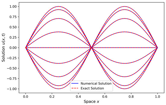
Figure 1.
Comparison of numerical and exact solutions.
4.2. Comparison with Existing Method
In this section we discuss the comparison of the explicit and implicit finite difference methods (FDM) analyzed with the established spectral and finite element methods (FEM). In terms of accuracy, the finite difference methods provide second-order accuracy + , whereas the spectral methods achieve exponential convergence ) for smooth solutions due to their global basis functions. Finite element methods exhibit accuracy, where is the mesh size and is the polynomial degree, offering flexibility in handling irregular geometries. Stability-wise, explicit FDM is constrained by the CFL condition , while implicit FDM is unconditionally stable but computationally more expensive. Spectral methods depend on the stability of the time integration scheme, such as Runge–Kutta, while FEM stability is influenced by the mesh design and stabilization techniques.
In spectral methods, the solution to the wave equation is approximated as a series expansion in terms of globally defined basis functions, such as the Fourier series or Chebyshev polynomials, with more details in [43]. The solution is expressed as
where are time-dependent coefficients, and are the basis functions. Spectral methods provide exponential convergence for smooth solutions, making them ideal for periodic problems. After projection onto these basis functions, the wave equation leads to a system of ODEs
where , represents the frequency of the -th mode. This system is solved using time-integration methods such as Runge–Kutta, which we observed to provide a high accuracy for smooth solutions, particularly suited for problems with periodic boundary conditions or smooth initial conditions.
The finite element method approximates the solution by discretizing the domain into smaller elements and solving the wave equation in weak form, with more details in [44]. The solution is approximated as
where are the piecewise polynomial shape functions. Applying the weak form of the wave equation and discretizing both space and time, we obtain the following system
where is the mass matrix, is the stiffness matrix, and is the vector of time-dependent coefficients. Time integration is performed using Newmark’s method, which is unconditionally stable and allows for larger timesteps, providing flexibility for complex geometries and large-scale simulations
Table 1 shows the comparison of the numerical methods.

Table 1.
Comparison of numerical methods.
The table shows that explicit FDM is efficient but limited by the CFL condition. Implicit FDM is stable for larger timesteps, though is computationally more expensive. Spectral methods offer high accuracy for smooth solutions but require sophisticated integration techniques. FEM is versatile for complex geometries but comes with higher computational costs.
4.3. Analyzing Norm of Error
The error is a measure of the difference between two sets of data, typically used to quantify the accuracy of a numerical method compared to an exact solution.
Figure 2 presents the evolution of the maximum of norm across all timesteps, demonstrating the convergence of numerical simulations towards the exact solution of the wave equation as the grid resolution increases. For each timestep , the norm of the error is computed as
where is the numerical solution and is the exact solution at the spatial point and timestep . Table 2 shows the order of accuracy vs. grid points of error analysis.
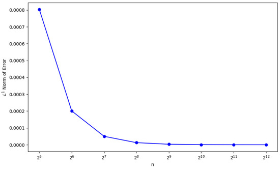
Figure 2.
Evolution of maximum norm of error over timesteps.
Table 2.
Order of accuracy vs. grid points.
4.4. Proof of Convergence
We establish convergence using the Lax–Richtmyer equivalence theorem, which states that a consistent and stable numerical scheme for a well-posed linear problem is convergent. We want to show that error converges to if To analyze the truncation error, we substitute the exact solution into the numerical scheme. Expanding and in Taylor series around we obtain the following expression for the time terms
Similarly, expanding and in Taylor series around , we obtain the following space expansions
Substituting these into our numerical scheme and comparing it with the discretized form of Equation , the truncation error can be found as
Thus, the truncation error tends towards zero as proving the consistency of our numerical scheme.
4.5. Analysis of Convergence
In this section, we investigate the convergence behavior of the finite difference method implemented to our governing equation. We seek to validate the accuracy and efficiency of our numerical solver by looking at the maximum error and the order of convergence for several grid resolutions. By means of numerical solution comparison with accurate analytical solutions, one can determine the maximum error at every grid resolution. Here, in our computation, we observed third-order convergence, which demonstrates the efficiency and robustness of our numerical scheme for solving the one-dimensional wave equation.
The proposed numerical scheme for the one-dimensional wave equation achieves third-order convergence through the careful design of temporal and spatial discretization. The second-order time derivative is approximated using a central finite difference scheme
which ensures a temporal accuracy of . For spatial discretization, a higher order finite difference formula is used for the second derivative
achieving accuracy in space. Combining these, the fully discretized scheme is expressed as
The truncation error analysis confirms that the scheme is dominated by terms of in time and in space. This balance enables the scheme to achieve third-order convergence under the CFL condition . To validate this theoretical result, we tested the scheme using a smooth analytical solution , where over different grid resolutions in Figure 3. The error norm was computed, and the observed convergence rate was determined as
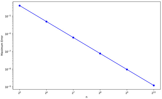
Figure 3.
Log-log plot of the maximum error versus the number of intervals
The results reveal a constant declining maximum error as the number of intervals n rises. More precisely, the error decreases by around a factor of eight with every twofold increase in n. The order of convergence computed between the consecutive values of is regularly around , so this pattern points to a third-order convergence. Table 3 summarizes the convergence rate results.
Table 3.
Third-order convergence.
4.6. Analysis of Relative Error
In this part, we investigate the relative error of the finite difference method implemented on the wave equation. We aim to grasp the accuracy of our numerical solver all through the simulation by analyzing the highest relative error at every timestep.
We compute the relative error in the norm defined by
where is the exact solution and is the numerical solution computed by the centered difference scheme. The Figure 4 give the maximum relative error as following.
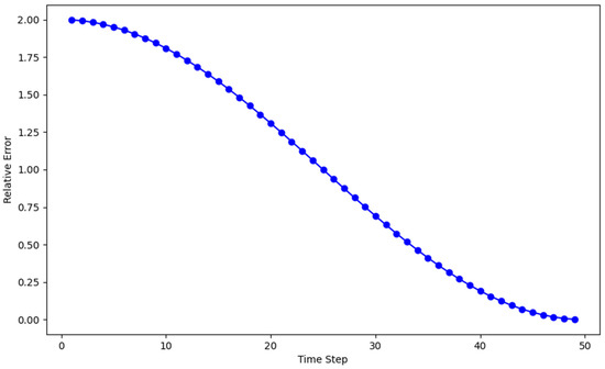
Figure 4.
Maximum relative error at each timestep.
The minimal relative error across timesteps shows that the finite difference method solves the wave equation with a great degree of accuracy. This study verifies the robustness of the numerical method by obtaining dependable results quite similar to the exact analytical solutions.
4.7. Proof of Stability Using Von Neumann Method
Stability analysis examines how numerical errors propagate over time. We decompose the numerical solution into Fourier modes of the form
where is the amplification factor, is the wave number, and represents a spatial Fourier mode.
We substitute in our numerical scheme to obtain the following simplified form
By factoring out , we have
Using the trigonometric identity , this reduces to the following
Now, let so then
For stability, we require which holds if . To satisfy this, it must hold that
We simplify the condition as follows:
Since for all , the stability condition reduces to
Thus, the proof of stability of our numerical scheme is as follows:
4.8. Numerical Results of Stability
In our work, we tested both explicit and implicit numerical schemes to assess their stability. For the explicit scheme, we carefully analyzed its behavior by adjusting parameters such as the timestep and resolution. We have shown proof of the stability analysis for our scheme in Section 4.7. We checked the numerical behavior of our scheme as if the solution remained bound and did not exhibit uncontrollable growth or oscillations over time. During these tests, we confirmed that, under the conditions developed in Section 4.7, the explicit scheme maintains stability, with the solution evolving smoothly without unphysical fluctuations. However, we also explored scenarios where instability could arise, particularly when larger timesteps or inappropriate resolutions were chosen. In such cases, the solution showed signs of divergence, such as erratic growth or oscillations, which confirmed the sensitivity of the explicit scheme to timestep size and other numerical parameters.
In addition to the explicit scheme, we also tested the implicit scheme numerically, which behaves unconditionally stable. Unlike the explicit scheme, the implicit scheme does not show any instability, regardless of the timestep size. This is because the implicit scheme allows for larger timesteps while ensuring that the solution remains stable and does not diverge. We performed a series of tests to verify this unconditional stability, and our results consistently showed that the implicit scheme maintained a stable solution even with very large timesteps. This makes the implicit scheme particularly advantageous for simulations requiring larger timesteps without risking instability, providing greater flexibility and robustness compared to the explicit scheme.
Morales-Hernandez et al. (2012) also show the same stability criteria as that which we derived for the one-dimensional wave equation, which is , and proposed an approach that allows for larger timesteps while maintaining accuracy in solving systems of conservation laws, such as shallow water equations, by incorporating strategies to control the stability when source terms or discontinuities are present [45].
The technique produces stability when the values of are less than 1; the amplitude of the solution does not develop uncontrollably over time; and the wave propagates without generating non-physical oscillations or distortions. Nevertheless, the explicit scheme becomes unstable if the CFL number is higher than 1. The exponential growth of the amplitude of the solution causes divergence and makes the simulation physically useless. Figure 5, Figure 6 and Figure 7 indicate the outcomes.
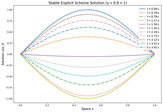
Figure 5.
Stable solution for explicit scheme satisfying CFL conditions .
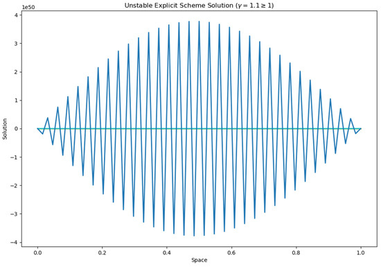
Figure 6.
Unstable solution for explicit scheme violating CFL conditions .
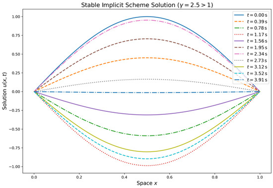
Figure 7.
Stable solution for implicit scheme for CFL number .
Figure 5 shows the numerical solution from the explicit scheme over time (in seconds). The spatial domain is discretized, and the solutions at key time points are shown, highlighting the evolution of the solution over time. Figure 6 shows an unstable solution from the same explicit scheme, showing instability as the CFL condition is exceeded. Figure 7 also violates the CFL condition, and the solution is still stable. This ensures that implicit scheme is unconditionally stable and that we choose larger timesteps for the computation. The spatial domain is discretized, and the solutions at key time points illustrate the scheme’s stability. The initial condition is considered as for all of the above three cases with both spatial and time domain units.
5. Conclusions
Using both explicit and implicit finite difference systems, this work has given a thorough investigation of numerical solutions to the one-dimensional wave equation. We have verified the great precision of the numerical methods applied by means of thorough error analysis comprising evaluations of the norm and relative errors. With the rate of convergence clearly measured, our convergence experiments show that the solutions converge successfully to the exact analytical solution as the discretization settings are improved. Using the von Neumann approach, the stability of both numerical systems has been extensively verified to guarantee consistent performance over simulations.
In Figure 1, we present a comparison between the exact and numerical solutions which shows a very close match, with the error being negligible. This indicates that the numerical method accurately approximates the exact solution. Figure 2 illustrates the norm of the error, demonstrating that the error decays rapidly as the resolution increases. After reaching a resolution of , the error becomes almost zero, confirming the good convergence rate of the scheme. Figure 3 presents a log-log plot of the maximum error against the resolution, where a constant decay is observed in the graph. This suggests that the error decreases at a consistent rate, which is typical for well-posed numerical schemes, indicating reliable and steady convergence. In Figure 4, the maximum relative error for each timestep is shown, and it decreases as expected, validating the stability and accuracy of the method over time. Figure 5 and Figure 6 demonstrate that the scheme satisfies the stability criterion, further confirming the robustness and reliability of the numerical approach. Lastly, Figure 7 shows that the scheme is unconditionally stable, as it is based on an implicit finite difference method. This unconditionally stable nature allows us to choose the timestep size freely, without worrying about stability constraints, further reinforcing the flexibility and effectiveness of the numerical scheme.
Author Contributions
Conceptualization, M.J.A., M.S.A., K.E.-R., M.T.A. and M.M.M.; Formal analysis, A.R. and M.T.A.; Investigation, M.J.A., M.S.A. and M.M.M.; Methodology, A.R.; Software, M.J.A., K.E.-R. and M.M.M.; Supervision, M.J.A.; Validation, A.R.; Writing—original draft, A.R., M.S.A., K.E.-R. and M.T.A.; Writing—review and editing, M.J.A. and M.M.M. All authors have read and agreed to the published version of the manuscript.
Funding
This research received no external funding.
Data Availability Statement
All data generated or analyzed during this study are included in this article.
Acknowledgments
The authors would like to acknowledge Deanship of Graduate Studies and Scientific Research, Taif University for funding this work.
Conflicts of Interest
The authors declare no conflicts of interest.
References
- Mead, D.J. Wave Propagation and Natural Modes in Periodic Systems: II. Multi-Coupled Systems, With and Without Damping. J. Sound Vib. 1975, 40, 19–39. [Google Scholar] [CrossRef]
- Sepahvand, K.; Marburg, S.; Hardtke, H.-J. Numerical solution of one-dimensional wave equation with stochastic parameters using generalized polynomial chaos expansion. J. Comput. Acoust. 1975, 15, 579–593. [Google Scholar] [CrossRef]
- Gu, M.H.; Young, D.L.; Fan, C.M. The method of fundamental solutions for one-dimensional wave equations. Tech Sci. Press CMC 2009, 11, 185–208. [Google Scholar]
- Wazwaz, A.M. One Dimensional Wave Equation. In Nonlinear Physical Science (NPS), Chapter: Partial Differential Equations and Solitary Waves Theory; Springer: Berlin/Heidelberg, Germany, 2010; pp. 143–194. [Google Scholar]
- Nicaise, S.; Pignotti, C. Stability and instability results of the wave equation with a delay term in the boundary or internal feedbacks. SIAM J. Control Optim. 2006, 45, 1561–1585. [Google Scholar] [CrossRef]
- Gao, R.; Ralescu, D.A. Uncertain Wave Equation for Vibrating String. IEEE Trans. Fuzzy Syst. 2019, 27, 1323–1331. [Google Scholar] [CrossRef]
- Leckar, H.; Sampaio, R.; Cataldo, E. Validation of the D’Alembert’s equation for the vibrating string problem. Trends Comput. Appl. Math. 2006, 7, 75–84. [Google Scholar] [CrossRef]
- Alabdali, F.M.; Bakodah, H.O. A New Modification of the Method of Lines for First Order Hyperbolic PDEs. Appl. Math. 2014, 5, 1457–1462. [Google Scholar] [CrossRef]
- Smith, G.D. Numerical Solution of Partial Differential Equations: Finite Difference Methods, 3rd ed.; Oxford University Press: Oxford, UK, 1985. [Google Scholar]
- Azam, T.; Pandit, M.K.; Andallah, L.S. Numerical Simulation of a Second Order Traffic Flow Model. GANIT J. Bangladesh Math. Soc. 2014, 34, 101–110. [Google Scholar] [CrossRef][Green Version]
- Ali, M.S.; Andallah, L.S.; Begum, M. Numerical Study of a Fluid Dynamic Traffic Flow Model. Int. J. Sci. Eng. Res. 2018, 9, 1092–1098. [Google Scholar]
- Kreiss, H.-O.; Petersson, N.A.; Yström, J. Difference Approximations for the Second Order Wave Equation. SIAM J. Numer. Anal. 1997, 34, 575–592. [Google Scholar] [CrossRef]
- Chabassier, J.; Joly, P. Energy preserving schemes for nonlinear Hamiltonian systems of wave equations: Application to the vibrating piano string. Comput. Methods Appl. Mech. Eng. 2010, 199, 2779–2795. [Google Scholar] [CrossRef]
- Aleroev, T.S.; Elsayed, A.M. Analytical and Approximate Solution for Solving the Vibration String Equation with a Fractional Derivative. Mathematics 2020, 8, 1154. [Google Scholar] [CrossRef]
- Chen, L.-Q.; Ding, H. Two nonlinear models of a transversely vibrating string. Arch. Appl. Mech. 2008, 78, 321–328. [Google Scholar] [CrossRef]
- Cumber, P.S. Application of the method of lines to the wave equation for simulating vibrating strings. Int. J. Math. Educ. Sci. Technol. 2024. [Google Scholar] [CrossRef]
- Bilbao, S.; Ducceschi, M. Models of musical string vibration. Acoust. Sci. Technol. 2023, 44, 194–209. [Google Scholar] [CrossRef]
- Zabusky, N.J. Exact solution for the vibrations of a nonlinear continuous model string. J. Math. Phys. 1962, 3, 1028–1039. [Google Scholar] [CrossRef]
- Ducceschi, M.; Bilbao, S. Linear stiff string vibrations in musical acoustics: Assessment and comparison of models. J. Acoust. Soc. Am. 2016, 140, 2445–2454. [Google Scholar] [CrossRef]
- Georg Schmidt, E.J.P. On the modelling and exact controllability of networks of vibrating strings. SIAM J. Control Optim. 1992, 30, 230–245. [Google Scholar] [CrossRef]
- Bensa, J.; Bilbao, S.; Kronland-Martinet, R.; Smith, J.O., III. The simulation of piano string vibration: From physical models to finite difference schemes and digital waveguides. J. Acoust. Soc. Am. 2003, 114, 1095–1107. [Google Scholar] [CrossRef] [PubMed]
- Park, J.; Kang, N. Applications of fiber models based on discrete element method to string vibration. J. Mech. Sci. Technol. 2009, 23, 372–380. [Google Scholar] [CrossRef]
- Mihalache, B.; Berlic, C. Using Excel spreadsheets to study the vibrating string behavior. Rom. Rep. Phys. 2018, 70, 901. [Google Scholar]
- Medeiros, L.A.; Limaco, J.; Menezes, S.B. Vibrations of elastic strings: Mathematical aspects, Part One. J. Comput. Anal. Appl. 2002, 4, 91–127. [Google Scholar]
- Carrou, J.-L.; Gautier, F.; Dauchez, N.; Gilbert, J. Modelling of sympathetic string vibrations. Acta Acust. United Acust. 2005, 91, 277–288. [Google Scholar] [CrossRef]
- Chaigne, A.; Askenfelt, A. Numerical simulations of piano strings. I. A physical model for a struck string using finite difference methods. J. Acoust. Soc. Am. 1994, 95, 1112–1118. [Google Scholar] [CrossRef]
- Chaigne, A.; Doutaut, V. Numerical simulations of xylophones. I. Time-domain modeling of the vibrating bars. J. Acoust. Soc. Am. 1997, 101, 539–557. [Google Scholar] [CrossRef]
- Chen, L.-Q. Analysis and Control of Transverse Vibrations of Axially Moving Strings. Appl. Mech. Rev. 2005, 58, 91–116. [Google Scholar] [CrossRef]
- Bank, B.; Sujbert, L. Generation of longitudinal vibrations in piano strings: From physics to sound synthesis. J. Acoust. Soc. Am. 2005, 117, 2268–2278. [Google Scholar] [CrossRef]
- Sahoo, S.; Das, H.C.; Panda, L.N. An Overview of Transverse Vibration of Axially Travelling String. In Recent Trends in Applied Mathematics; Springer: Singapore, 2021; pp. 427–446. [Google Scholar]
- Argudo, D.; Oh, T. A new framework to study the wave motion of flexible strings in the undergraduate classroom using linear elastic theory. Eur. J. Phys. Educ. 2022, 13, 10–29. [Google Scholar]
- Auret, F.D.; Snyman, J.A. Numerical study of linear and nonlinear string vibrations by means of physical discretization. Appl. Math. Model. 1978, 2, 7–17. [Google Scholar] [CrossRef]
- Lee, S.-Y.; Lee, M. A new wave technique for free vibration of a string with time-varying length. J. Appl. Mech. 2002, 69, 83–87. [Google Scholar] [CrossRef]
- Miska, S.Z.; Zamanipour, Z.; Merlo, A.; Porche, M.N. Dynamic soft string model and its practical application. In Proceedings of the SPE/IADC Drilling Conference and Exhibition, London, UK, 17–19 March 2015. [Google Scholar] [CrossRef]
- Selvadurai, A.P.S. The wave equation. In Partial Differential Equations in Mechanics 1; Springer: Berlin/Heidelberg, Germany, 2001; pp. 369–555. [Google Scholar]
- Kaselouris, E.; Bakarezos, M.; Tatarakis, M.; Papadogiannis, N.A.; Dimitriou, V. A review of finite element studies in string musical instruments. Acoustics 2022, 4, 183–202. [Google Scholar] [CrossRef]
- Pakdemirli, M.; Ulsoy, A.G.; Ceranoglu, A. Transverse vibration of an axially accelerating string. J. Sound Vib. 1994, 169, 179–196. [Google Scholar] [CrossRef]
- Mounier, H.; Rudolph, J.; Fliess, M.; Rouchon, P. Tracking control of a vibrating string with an interior mass viewed as delay system. ESAIM Control Optim. Calc. Var. 2002, 3, 315–321. [Google Scholar] [CrossRef]
- Grimes, D.R. String theory — The physics of string-bending and other electric guitar techniques. PLoS ONE 2014, 9, e102088. [Google Scholar] [CrossRef]
- Ahn, J. A vibrating string with dynamic frictionless impact. Appl. Numer. Math. 2007, 57, 861–884. [Google Scholar] [CrossRef]
- Gimperlein, H.; Oberguggenberger, M. Solutions to semilinear wave equations of very low regularity. J. Differ. Equ. 2024, 406, 302–317. [Google Scholar] [CrossRef]
- Park, S.-H.; Kang, J.-R. Stability analysis for wave equations with variable exponents and acoustic boundary conditions. Math. Methods Appl. Sci. 2024, 47, 14476–14486. [Google Scholar] [CrossRef]
- Hussaini, M.Y.; Zang, T.A. Spectral Methods in Fluid Dynamics. Annu. Rev. Fluid Mech. 1987, 19, 339–367. [Google Scholar] [CrossRef]
- Richter, G.R. An explicit finite element method for the wave equation. Appl. Numer. Math. 1994, 16, 65–80. [Google Scholar] [CrossRef]
- Morales-Hernandez, M.; García-Navarro, P.; Murillo, J. A large time step 1D upwind explicit scheme (CFL > 1): Application to shallow water equations. J. Comput. Phys. 2012, 231, 6335–6354. [Google Scholar] [CrossRef]


Disclaimer/Publisher’s Note: The statements, opinions and data contained in all publications are solely those of the individual author(s) and contributor(s) and not of MDPI and/or the editor(s). MDPI and/or the editor(s) disclaim responsibility for any injury to people or property resulting from any ideas, methods, instructions or products referred to in the content. |
© 2025 by the authors. Licensee MDPI, Basel, Switzerland. This article is an open access article distributed under the terms and conditions of the Creative Commons Attribution (CC BY) license (https://creativecommons.org/licenses/by/4.0/).