Abstract
It is widely believed that one of the main causes of the replication crisis in scientific research is some of the most commonly used statistical methods, such as null hypothesis significance testing (NHST). This has prompted many scientists to call for statistics reform. As a practitioner in hydraulics and measurement science, the author extensively used statistical methods in environmental engineering and hydrological survey projects. The author strongly concurs with the need for statistics reform. This paper offers a practitioner’s perspective on statistics reform. In the author’s view, some statistical methods are good and should withstand statistics reform, while others are flawed and should be abandoned and removed from textbooks and software packages. This paper focuses on the following two methods derived from the t-distribution: the two-sample t-test and the t-interval method for calculating measurement uncertainty. We demonstrate why both methods should be abandoned. We recommend using “advanced estimation statistics” in place of the two-sample t-test and an unbiased estimation method in place of the t-interval method. Two examples are presented to illustrate the recommended approaches.
1. Introduction
In recent years, the scientific community has become increasingly concerned about the replication crisis. Many scientists believe that one of main causes of the replication crisis is some of the most commonly used statistical methods. Specifically, null hypothesis significance testing (NHST) and its produced p-values, and claims of statistical significance, have come in most to blame [1]. Hirschauer et al. [2] reviewed the history and explained “how it came that the meaningful signal and noise information that can be extracted from a random sample was distorted almost beyond recognition into statistical significance declarations”. Siegfried [3] remarked, “It’s science’s dirtiest secret: The ‘scientific method’ of testing hypotheses by statistical analysis stands on a flimsy foundation”. Siegfried [4] further claimed, “statistical techniques for testing hypotheses …have more flaws than Facebook’s privacy policies”.
In response to these concerns, many scientists have called for the retirement or abandonment of statistical significance and p-values (e.g., [5,6,7,8,9]). For instance, since 2015, Basic and Applied Social Psychology has banned NHST procedures and p-values [10]. Furthermore, many scientists have advocated for statistics reform (e.g., [11,12,13]). Amrhein and Greenland [14] stated, “… we think statistics reform should involve completely discarding ‘significance’ and the oversimplified reasoning it encourages, instead of just shifting thresholds”. Cumming [15] and Cumming and Calin-Jageman [16] proposed the “New Statistics”, which primarily involves (1) abandoning NHST procedures and (2) using effect sizes and confidence intervals. Normile et al. [17] introduced the “New Statistics” in classroom settings. Claridge-Chang and Assam [18] suggested replacing significance testing with estimation statistics. A co-published editorial of 14 physiotherapy journals [19] “… advises researchers that some physiotherapy journals that are members of the International Society of Physiotherapy Journal Editors (ISPJE) will be expecting manuscripts to use estimation methods instead of null hypothesis statistical tests”. More recently, Trafimow et al. [20,21] proposed using a two-step process comprising the APP (a priori procedure) and gain-probability analyses to replace the traditional two-step process comprising the power analysis and NHST. Although some authors continue to defend NHST and p-values (e.g., [22,23,24]), and the debate persists (e.g., [25,26]), Berner and Amrhein [27] noted that “A paradigm shift away from null hypothesis significance testing seems in progress”.
As a practitioner in hydraulics and measurement science, the author extensively used statistical methods in environmental engineering and hydrological survey projects (citation omitted). In particular, the author processed thousands of small samples collected during streamflow measurements using acoustic Doppler current profilers (ADCPs). Typically, an ADCP streamflow measurement involves only a few observations (usually around four). According to the Guide to the Expression of Uncertainty in Measurement (GUM; [28]), the uncertainty of the sample mean from a small sample should be calculated using the t-interval method. However, the author found that the t-based uncertainty (i.e., the half-width of the t-interval) was unrealistic and misleading, leading to the so-called “uncertainty paradox” [29,30] and a high false rejection rate in the quality control of ADCP streamflow measurements [31].
The author is not alone in questioning the validity of the t-interval method for calculating measurement uncertainty. Jenkins [32] also found that the t-based uncertainty can exhibit significant bias and precision errors. D’Agostini [33] provided the following striking example: “…having measuring the size of this page twice and having found a difference of 0.3 mm between the measurements… Any rational person will refuse to state that, in order to be 99.9% confidence in the result, the uncertainty interval should be 9.5 cm wide (any carpenter would laugh…). This may be the reason why, as far as I known, physicists don’t use the Student distribution”. Furthermore, Ballico [34] reported a notable counterinstance during a routine calibration at the CSIRO National Measurement Laboratory (NML), Australia. In this instance, a thermometer was calibrated for a 1 mK range (higher precision) and a 10 mK range (lower precision); the uncertainty was calculated using the WS-t approach (which combines the Welch–Satterthwaite formula with the t-interval). Intuitively, one would expect the thermometer in the higher precision range to have a lower uncertainty than in the lower precision range. However, the WS-t approach gave a counterintuitive result: the uncertainty for the 1 mK range was 37.39, compared to 35.07 for the 10 mK range. This counterintuitive result became known as the Ballico paradox [35].
Practitioners in science and industry rely on statistical methods in their work, and the use of flawed methods can have significant negative impacts. Ziliak and McCloskey [36] demonstrated in their extensive 322-page volume that “Statistical significance is an exceptionally damaging one.” However, over the years, the author has observed that practitioners are frequently accused of misunderstanding and misusing certain statistical methods, particularly NHST procedures and p-values, even though the root issue may lie with the methods themselves. In the author’s view, if a statistical method or concept is so prone to misunderstanding and misusing that even educational institutions struggle to teach it effectively, then there is likely something inherently wrong with that method or concept. Trafimow [37] argued that, “NHST is problematic anyway even without misuse”. And “There is practically no way to use them [p-values] properly in a way that furthers scientific practice”. While the debate about NHST procedures and p-values persists, one fact remains clear: after roughly 100 years, NHST procedures and p-values have not withstood the test of time.
We understand that no statistical method is perfect, nor can any method be applied without limitations or conditions. However, in the experience of the author and other practitioners, some statistical methods, such as the least squares method and point estimation, have proven to be good and useful. In contrast, other methods, such as the t-interval method for calculating measurement uncertainty, have demonstrated serious flaws. The coexistence of sound and problematic methods can be confusing to practitioners, many of whom may not realize that some methods are flawed or controversial and continue to use them inadvertently.
Therefore, the author strongly concurs with the need for statistics reform. This paper offers a practitioner’s perspective on statistics reform. We argue that good methods should be preserved, while flawed methods should be abandoned and removed from textbooks and software packages. This paper focuses on the following two methods derived from the t-distribution: the two-sample t-test and the t-interval method for calculating measurement uncertainty. We will present arguments for why these two methods should be abandoned and propose alternatives.
The rest of the paper is organized as follows. Section 2 briefly reviews examples of good statistical methods that should withstand statistics reform. Section 3 discusses why the two-sample t-test should be abandoned, while Section 4 describes an alternative to this test. Section 5 discusses why the t-interval method for calculating measurement uncertainty should be abandoned, while Section 6 describes an alternative to the t-interval method. Section 7 provides conclusions and recommendations.
2. Examples of Good Statistical Methods That Should Withstand Statistics Reform
In the author’s opinion, a good statistical method should possess the following characteristics: (a) it should have clear mathematical meaning and be easily understood, even by those without advanced training in statistics; (b) it should yield realistic results in real-world applications; and (c) it should be relatively uncontroversial in the scientific community. Furthermore, ideally, a good statistical method would be related to a physical principle, thus giving it physical meaning. Many good statistical methods meet these criteria. Four examples are listed below.
- Method of least squares;
- Method of maximum likelihood;
- Central Limit Theorem;
- Akaike information criterion (AIC).
The least squares method is perhaps one of the widely used statistical methods in practice. It is hardly controversial in the scientific community and, importantly, it conforms to the principle of minimum energy, a fundamental concept in physics. In this context, the sum of squared errors can be interpreted as representing the internal noise energy of the system under consideration, which naturally tends to a minimum value at equilibrium.
The method of maximum likelihood is another widely used statistical method. It is also hardly controversial in the scientific community. The method of maximum likelihood is intuitive in nature; as Fisher [38] stated, “The likelihood supplies a natural order of preference among the possibilities under consideration”. In other words, the mode of a likelihood function corresponds to the most preferred parameter value given the data [39]. This idea is straightforward and does not require advanced statistical knowledge to understand. In addition, the method of maximum likelihood is essentially consistent with the least squares method.
The Central Limit Theorem states that, given a sufficiently large sample size, the sampling distribution of the sample mean will approximate a normal distribution, regardless of the original distribution. Since measurement error is defined as the difference between the true value and the measured value (e.g., the sample mean), the Central Limit Theorem aligns with the law of error, which is one of the foundational principles in statistics and measurement science.
The Akaike information criterion (AIC) is based on the concept of entropy in information theory. A model with the minimum AIC minimizes information loss among a set of candidate models. Essentially, the AIC is consistent with the maximum likelihood method and the least squares method.
Of course, good statistical methods like the four motioned above should withstand statistics reform.
3. Why Should the Two-Sample t-Test Be Abandoned?
The two-sample t-test is perhaps the most widely used procedure among NHST procedures. Therefore, if we are to abandon NHST procedures, the two-sample t-test should be abandoned first. However, the literature rarely provides an explicit discussion of the reasons for abandoning the two-sample t-test, and usually offers only general debates about the problems with NHST procedures and p-values. It is important to note that p-values are outputs of statistical methods such as the two-sample t-test. Thus, p-value problems are not solely with p-values but with the statistical methods that produce them. In this section, we address the following two main issues with the two-sample t-test: logic and performance. We argue that these shortcomings provide compelling reasons for its abandonment.
3.1. Logic Issue: The Two-Sample t-Test Is Philosophically Flawed and Misleading
The two-sample t-test is philosophically flawed and misleading. Consider the following two datasets (groups): Group A from treatment A and Group B from treatment B. We are interested in determining whether treatment A is superior to treatment B (or vice versa). In the standard NHST framework, we begin with a null hypothesis, a “strawman”, that the unknown population means of the two groups are the same, and an alternative hypothesis that they differ. Then, we use the two-sample t-test to generate a p-value. If p < 0.05, we conclude that the deference between the two means is “statistically significant” and the null hypothesis is rejected, i.e., the “strawman” is disproven. However, this approach does not answer the question of superiority between treatments A and B. Instead, it misleads us to focus on whether the groups differ in a statistically significant manner based on an arbitrary p-value threshold. In reality, simply examining the data or comparing the group means often suffices to show that treatment A is different from treatment B. We should directly assess the practical importance of the observed difference using our domain knowledge. There is no intrinsic need to construct a “strawman” (the null hypothesis) and then try to disprove it.
3.2. Performance Issues: Uncertainty, Inconsistency, and Dependence on Sample Size
Even if we accept its logic and use it for comparing the means of two groups, the two-sample t-test does not provide reliable results. This can be understood by examining the behaviors of the p-value produced by the test. First, as with any sample statistics, the p-value itself is subject to uncertainty. Halsey et al. [40] discussed the uncertainty associated with the p-value of two-sample t-tests through simulations. They demonstrated that “a major cause of the lack of repeatability is the wide sample-to-sample variability in the p value”. They stated that, “As we have demonstrated, however, unless statistical power is very high (and much higher than in most experiments), the p value should be interpreted tentatively at best. Data analysis and interpretation must incorporate the uncertainty embedded in a p value”. Hirschauer et al. [41] pointed out that “The p-value’s variability over replications undermines its already weak informative value”. Moreover, Lazzeroni et al. [42] introduced p-value confidence intervals for the “true population p value” or π value, which they defined as the value of p when parameter estimates equal their unknown population values. They emphasized that “p values are variable, but this variability reflects the real uncertainty inherent in statistical results”.
Second, the two-sample t-test may produce inconsistent results for essentially the same evidence. Bonovas and Daniele [43] illustrated this issue with two trials of a new drug. In a single-center, randomized, double-blind, placebo-controlled trial, the two-sample t-test produced a p-value of 0.11, suggesting “no difference” between the active drug and placebo. In contrast, a multi-center trial yielded a p-value of 0.001, indicating a “significant difference”. Despite these conflicting p-values, the risk ratio was the same in both trials, 0.70, indicating that the efficacy of the experimental drug was the same. This discrepancy highlights a critical shortcoming of the two-sample t-test: its reliance on p-values can lead to inconsistent and potentially misleading conclusions, even when the effect size is consistent.
Third, the p-value produced by a two-sample t-test is highly dependent on the sample size; it decreases as the sample size increases. Therefore, p-values can be easily “hacked” through “N-chasing” (a term coined by Stansbury [44]), which guarantees “statistical significance” at any pre-specified threshold even if the effect size (e.g., the difference between the means of two groups) is trivial and lacks practical significance. “N-chasing” is one of the most effective ways of p-hacking. In the author’s opinion, the only viable solution to combat “N-chasing” or p-hacking is to abandon the two-sample t-test.
4. Alternative to the Two-Sample t-Test: Advanced Estimation Statistics
We recommend using advanced estimation statistics in place of the two-sample t-test. This framework emphasizes a comprehensive presentation of a set of statistics, including the observed effect size (ES), relative effect size (RES), standard uncertainty (SU), relative standard uncertainty (RSU), signal-to-noise ratio (SNR), signal content index (SCI), exceedance probability (EP), and net superiority probability (NSP). Each of these eight statistics has a clear mathematical or physical meaning and is easy to understand.
In this advanced estimation statistics framework, the superiority of treatment A over treatment B (or vice versa) is measured by the observed ES (or RES) along with the EP (or NSP). The uncertainty of the observed ES (or RES) is assessed using the SU or RSU, while the reliability of the observed ES (or RES) is assessed using the SNR or SCI. We will make scientific inferences based on domain knowledge and taking these statistics into account, rather than purely statistical inferences.
Moreover, this advanced estimation statistics framework avoids the terminology and language associated with the NHST paradigm. Terms such as null hypothesis, alternative hypothesis, p-values, statistical significance, and statistical power are eliminated.
4.1. Observed Effect Size (ES) and Relative Effect Size (RES)
The observed effect size (ES), denoted by , is defined as the absolute deference between the two group means ( and , respectively), as follows:
It is important to note that the observed ES represents the “simple” effect size. It is the raw difference between the means of two groups, expressed in the original physical unit of the quantity of interest. This is in contrast to standardized effect sizes, such as Cohen’s d, which is dimensionless. Because the simple effect size retains the original physical unit, it is nearly always more meaningful than the standardized effect size [45]. Schäfer [46] argued that, in their unstandardized form, effect sizes are easy to calculate and to interpret. Standardized effect sizes, on the other hand, bear a high risk for misinterpretation. In real-world applications, practitioners’ domain knowledge is inherently tied to the physical units of the quantity of interest. Therefore, it is more intuitive for practitioners to assess the practical significance using simple effect sizes. As Baguley [45] noted, “For most purposes simple (unstandardized) effect size is more robust and versatile than standardized effect size”. Therefore, we do not recommend using standardized effect sizes such as Cohen’s d in the advanced estimation statistics framework.
Note also that the observed ES represents the absolute magnitude of the treatment effect. In practice, we are often interested in the relative magnitude of the treatment effect, i.e., the relative effect size (RES). According to Huang [39], the RES is defined as the ratio of the observed ES to a baseline measure, such as the average of the two group means. That is
where can be calculated as the inverse-variance weighted-average, as follows:
where and ; and are the sample standard deviation of Group A and Group B, respectively; nA and nB are the sample size of Group A and Group B, respectively. The RES is usually expressed as a percentage.
The observed ES or RES is independent of the sample size. As such, it only emphasizes the treatment effect. Unlike the two-sample t-test, which confounds the treatment effect with the sample size, increasing the sample size does not alter the observed ES or RES but rather improves its reliability. Therefore, in contrast to p-values from t-tests, which are vulnerable to “N-chasing”, the observed ES or RES cannot be hacked through “N-chasing”.
4.2. Standard Uncertainty (SU), Relative Standard Uncertainty (RSU), Signal-to-Noise Ratio (SNR), and Signal Content Index (SCI)
The observed ES is a point estimate of the unknown true effect size. Its reliability must be quantified and assessed. To this end, statistics such as the standard uncertainty (SU), relative standard uncertainty (RSU), signal-to-noise ratio (SNR), and signal content index (SCI) are employed. These statistics collectively provide a comprehensive assessment of the reliability of the observed ES.
Let denote the SU of the observed ES . It is given by
In measurement science, is often used as a measure of the precision of a measurement. If we treat the observed ES as a measurement result, then measures its precision. Note that has the same physical unit as .
In practice, we are also interested in the relative standard uncertainty (RSU) (if applicable), defined as
The signal-to-noise ratio (SNR) is defined as the ratio of signal energy to noise energy. Although it is commonly used in electrical engineering, the concept applies to any signal [47]. For comparing the means of two groups, the observed ES represents the signal, while the SU represents the noise. Therefore, the SNR is given by
Moreover, the signal content index (SCI) is defined as [47]
The SCI has a clear physical meaning; it is the relative amount of signal energy contained in the measurement result [47].
It should be noted that, unlike the observed ES or RES, which is independent of the sample size, the reliability measures such as the SU, RSU, SNR, and SCI are functions of the sample size. As the sample size increases, the SU and RSU decrease, while the SNR and SCI increase. This establishes a clear distinction between the observed ES and its reliability measures.
It should also be noted that we do not use a confidence interval to quantify the uncertainty (or precision) of the observed ES. This is because the concept of confidence intervals has long been controversial and subject to debate in the scientific community (e.g., [48,49,50,51,52]). In particular, the t-interval, which is a confidence interval traditionally used for small samples, is problematic and, as discussed in Section 5, should be abandoned.
4.3. Exceedance Probability (EP) and Net Superiority Probability (NSP)
The observed ES measures the difference, on average, between the two treatments A and B. In other words, when we assume that , the observed ES quantifies the average superiority of treatment A over treatment B. However, in practice, we are also interested in assessing superiority at the individual level. This means comparing the individual scores in the two groups to determine how often individuals in Group A outperform those in Group B.
The probability that Group A is superior to Group B at the individual level is known as exceedance probability (EP) and is defined as [39]
where and represent the scores of individuals in Groups A and B, respectively, and is the probability density function for the quantity .
The exceedance probability is interpreted as the probability (or chance) that a randomly picked person from Group A will score higher than a randomly picked person from Group B.
On the other hand, we can calculate the probability that Group B is superior to Group A as follows: . If , Group A is considered superior to Group B; if , Group B is considered superior to Group A. In the case where , there is no superiority between Group A and Group B.
The meaning of the exceedance probability is essentially the same as that of several other statistics, including the common language effect size (CLES), the probability of superiority (PS), and the area under the receiver operating characteristic curve (AUC) or its non-parametric version (A). However, it is important to note that calculating the CLES requires assumptions of population normality and equal variances, whereas does not require these assumptions. In this sense, the CLES is an approximation of . Additionally, the term “CLES” can be misleading, as it might imply that it is an effect size, when in fact it represents a probability.
Assume that both and are normally distributed with unknown means and unknown variances. The estimated distributions of XA and XB are and , respectively, where is the bias correction factor, , and Γ(.) stands for the Gamma function. In addition, the estimated distribution of is also a normal distribution, as follows:
Then, the exceedance probability of is given by [53]
where is the cumulative distribution function of the standard normal distribution and is given by
The exceedance probability of is given by
Furthermore, the net superiority probability (NSP), denoted by , is related to the exceedance probabilities as [53]
Although Equation (13) is based on the normality assumption, it is considered as a general definition of the NSP for any types of distributions of XA and XB [53].
It is important to note that the EP or NSP is only a very weak function of sample sizes due to the bias correction factor . Therefore, similar to the observed ES or RES, the EP or NSP is resistant to manipulation via “N-chasing”.
The above probabilistic analyses rely on probability distributions. However, these analyses can also be performed without assuming specific distributions, in what is known as non-parametric comparison of two groups. In the distribution-free analysis, the exceedance probability is given by [53]
And the exceedance probability is given by
where or is the U statistic in the Mann–Whitney U test.
Accordingly, the NSP of Group A over Group B is given by
It should be noted that the concept of the exceedance probability (EP) is essentially equivalent to the gain-probability (G-P) proposed by Trafimow et al. [20,21]. Moreover, the EP and its analysis have been used across various engineering fields. For instance, the U.S. EPA [54] established a probabilistic chronic toxics standard of EP = 0.0037 to protect aquatic life. Di Toro [55] conducted an EP analysis of river quality affected by runoff. Huang and Fergen [56] applied EP analysis to assess river BOD (biochemical oxygen demand) and DO (dissolved oxygen) concentrations in response to point load. Krishnamoorthy et al. [57] also utilized EP analysis to assess exposure levels in work environments. Furthermore, the concept of exceedance probability is closely related to the term “return period” commonly used in hydraulic engineering and hydrology. For example, a 100-year flood corresponds to an exceedance probability of 1%. Therefore, practitioners in engineering fields are typically more familiar with the concept of exceedance probability than with terms like the CLES, AUC, or A.
4.4. A Flowchart of the Advanced Estimation Statistics Framework for Comparing Two Groups
Figure 1 shows a flowchart of the advanced estimation statistics framework for comparing the following two groups: A and B. We assume that Group A represents the treatment group in a controlled experiment and Group B represents the control group. The data corresponding Group A are X: {xA,1, xA,2, …, xA,nA} and the data corresponding Group B are X: {xB,1, xB,2, …, xB,nB}, where nA and nB are the sample sizes.
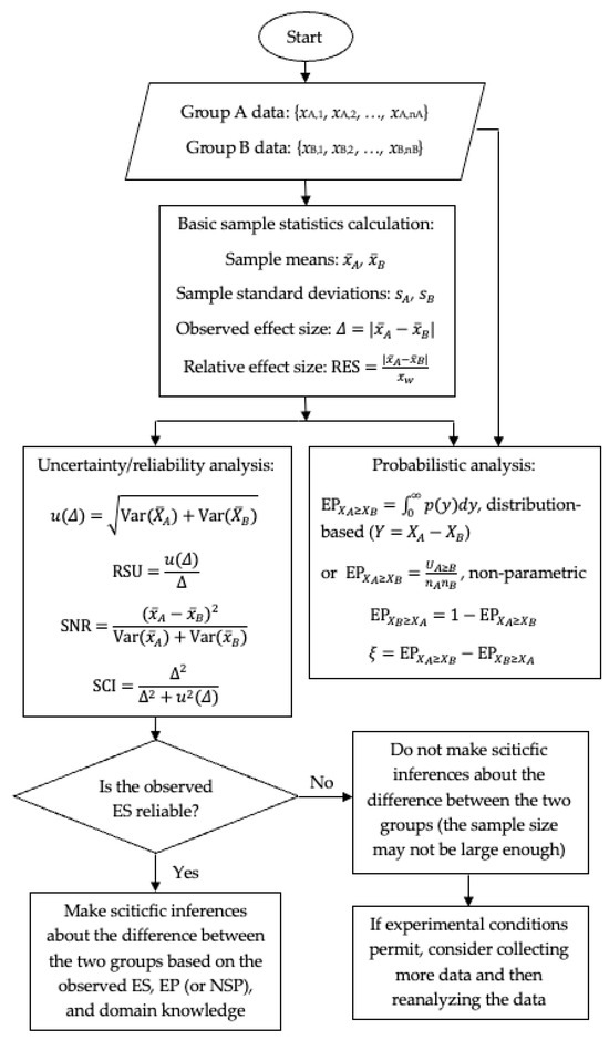
Figure 1.
Flowchart of the advanced estimation statistics framework for comparing two groups.
As shown in the flowchart, our analysis starts with calculating the following basic sample statistics: the sample mean, sample standard deviation, observed effect size (ES), and relative effect size (RES). We then perform the following two types of analyses: (1) uncertainty/reliability analysis, which gives the standard uncertainty (SU), relative standard uncertainty (RSU), signal-to-noise ratio (SNR), and signal content index (SCI); (2) probabilistic analysis, which gives the exceedance probability (EP) and net superiority probability (NSP). Note that the EP and NSP can be obtained based on the estimated distributions or using the non-parametric method.
It is important to note that we regard the observed ES as an estimate of the true effect size. We must make ensure that the observed ES is reliable and trustworthy. If the observed ES is unreliable, we cannot make correct scientific inferences. Therefore, before making scientific inferences, we must assess the uncertainty and reliability of the observed ES. The uncertainty of the observed ES is quantified by the SU or RSU and its reliability is quantified by the SNR or SCI. Since the SU, RSU, and SNR are unbounded quantities, their interpretations are not intuitive. In contrast, the SCI is bounded between 0 and 1, and its interpretation is intuitive. A high SCI value (e.g., close to 1) indicates that the observed ES is reliable, while a low SCI value (e.g., close to 0) indicates that the observed ES is unreliable. We propose (tentatively) to use SCI values of 0.25, 0.5, and 0.75 (corresponding to low, moderate, and high reliability, respectively) to assess the reliability of the observed ES. Note that these benchmarks are similar to those used in measurement science to assess the measurement validity or in meta-analysis to assess the between-study heterogeneity [47].
If the observed ES is determined to be reliable (for instance, if the SCI is greater than 0.75), we can make sciticfic inferences about the difference between the two groups based on the observed ES, the results of the probabilistic analysis, and our domain knowledge. If the observed ES is considered unreliable (for instance, if the SCI is smaller than 0.3), we should not make any firm inferences about the difference between the two groups. A low SCI value may suggest that the sample size is not sufficient. If the experimental conditions permit, we should collect more data and reanalyze.
In general, when the sample size is small, the observed ES (or any estimated parameter) is likely to be unreliable, even if the observed ES appears large. However, this raises the following question: “How unreliable is unreliable?” or “How low does an SCI value have to be considered unreliable?” While we recommend using the above SCI benchmarks to assess the reliability, we believe that the answer should ultimately be left to the researchers who design and conduct the experiment. For example, if a pilot study yields a high observed ES but a relatively low SCI due to a small sample size, the researchers should use their professional judgment to determine whether the observed ES is truly meaningful and warrants further investigation in a larger study.
4.5. Example: Comparison of Old and New Flavorings for a Beverage
Zaiontz [58] considered the following problem: a marketing research firm conducted experiments to evaluate the effectiveness of a new flavoring for a beverage. In the study, eleven people in Group A1 and ten people in Group A2 tasted the beverage with the new flavoring, while ten people in Group B tasted the beverage with the old favoring. After tasting, all of the participants took a questionnaire to evaluate how enjoyable the beverage was. The scores obtained for the new flavoring (Group A1 and Group A2) and old flavoring (Group B) are shown in Table 1, and the corresponding sample means and standard deviations are presented in Table 2.

Table 1.
Scores of the three groups in the beverage flavor taste experiments.
Table 2.
Sample means and standard deviations of the three groups in the beverage flavor taste experiments.
Zaiontz [58] applied the two-sample t-test (two-tailed) to compare the effectiveness of a new flavoring versus the old flavoring. For the comparison between Group A1 (new flavoring) and Group B (old flavoring), he obtained a p-value of 0.04, which led him to reject the null hypothesis at the α = 0.05 level and conclude that the new flavoring was significantly more enjoyable. However, for the comparison between Group A2 (new flavoring) and Group B (old flavoring), the p-value was 0.05773, and he could not reject the null hypothesis. It is peculiar that Zaiontz [58] did not address or comment on these contradictory results from the two t-tests.
We examined this example using the advanced estimation statistics. Table 3 shows the estimated effect sizes and their uncertainty and reliability measures. Table 4 shows the results of the probabilistic analysis based on the distribution-based comparison, while Table 5 shows the results based on the non-parametric comparison.
Table 3.
Estimated effect sizes and their reliability measures for the comparison of beverage flavoring.
Table 4.
Results of the probabilistic analysis based on the distribution-based comparison.
Table 5.
Results of the probabilistic analysis based on the non-parametric comparison.
As can be seen from Table 3, the observed ES is 3.81 and the RES is 28.52% for the comparison of Group A1 versus Group B, while the observed ES is 8.70 and the RES is 72.12% for the comparison of Group A2 versus Group B. Our domain knowledge and common sense in this case suggest that the difference between the two flavorings is practically significant. Although the RSUs are large (45.84% and 47.31%) due to the small sample sizes, the SNRs are high (4.76 and 4.47), and the SCIs are also high (0.83 and 0.82). These values indicate that the observed ES are reliable and that the experimental data are credible.
The estimated distributions of Y for the two comparisons can be seen from Table 4, showing that Group A1 versus Group B and Group A2 versus Group B are different, with for the former and for the latter. However, the difference in the values of the RSU, SNR, SCI, EP, and NSP between these two comparisons are small. Thus, the two comparisons should lead to the same conclusion: the new flavoring is superior to the old flavoring.
Note that the values of the EP and NSP from the distribution-based comparison (Table 4) are consistent with those obtained from the non-parametric comparison (Table 5). = 0.745, 0.742, and NSP = 0.490, 0.484 based on the distribution-based comparison, while = 0.741, 0.725, and NSP = 0.482, 0.450 based on the non-parametric comparison.
5. Why Should the t-Interval Method for Calculating Measurement Uncertainty Be Abandoned?
In measurement science, the half-width of the t-interval is defined as the Type A expanded uncertainty for a measurement with a small number of observations (e.g., [28]). It is referred to as the t-based uncertainty. In this section, we discuss the following two main issues with the t-interval and t-based uncertainty: rationale and methodology, which together explain why the t-interval method for calculating measurement uncertainty should be abandoned. We also examine problems associated with the t-distribution, which is the basis for the t-interval and t-based uncertainty.
5.1. Rationale Issue: “Coverage” Is a Misleading Concept
The rationale behind using the t-interval method for calculating measurement uncertainty is based on the concept of “coverage”. Coverage, expressed as the confidence level or coverage probability, is the central concept in Neyman confidence interval theory. However, it is important to note that the confidence level is not a probability in the strict mathematical sense; rather, it represents the “long-term success rate” (e.g., [59]) or “capture rate” [60]. In Monte Carlo simulation of the t-interval, the success or capture rate asymptotically approaches the nominal confidence level ). That is
where m is the total number of simulated t-intervals and k is the number of the intervals that capture the true value μ.
Therefore, strictly speaking, the confidence level is not a mathematical probability that satisfies Kolmogorov’s axioms of probability calculus; rather, it is a relative frequency. However, as Bunge [61] noted, “… frequencies alone do not warrant inferences to probabilities …” because “… whereas a probability statement concerns usually a single (though possible complex) fact, the corresponding frequency statement is about a set of facts and moreover as chosen in agreement with certain sampling procedures”. Bunge [61] further argued that “… the frequency interpretation [of probability] is mathematically incorrect because the axioms that define the probability measure do not contain the (semiempirical) notion of frequency”.
It is important to note that the “coverage” (the frequency of “success” or “capture”) is a property of the confidence interval procedure (e.g., the t-interval procedure). This coverage can only be realized in the long run through repeated sampling or simulation. For a confidence interval calculated from a sample, the probability that the “true” value is within the interval is 0 or 1.
We must distinguish between the result of a procedure and the coverage of the procedure. In measurement uncertainty analysis, our focus is on the estimated uncertainty given by the procedure. As Kempthorne [62] stated, “…a statistical method should be judged by the result which it gives in practice”. However, the concept of coverage does not represent a result produced by the method. Therefore, it is inappropriate and even paradoxical to judge an uncertainty estimation method by its coverage [63].
It should be emphasized that a confidence interval procedure is merely a mechanism to generate a collection of intervals (or “sticks”) with a stated capture rate for the unknown true value [60]. In other words, the t-interval method provides an “exact” answer to the following question: “What is the interval procedure with which the population mean μ would be captured by 1-α of all intervals generated in the long-run of repeated sampling?” However, this is the wrong question for measurement uncertainty analysis. The purpose of measurement uncertainty analysis is to determine (or estimate) the measurement precision with a given sample. The correct question is as follows: “How do we estimate measurement precision with a given sample?” [64]. In this context, the t-interval procedure is not an appropriate method for inferring measurement precision. Morey et al. [50] argued the following: “Claims that confidence intervals yield an index of precision, that the values within them are plausible, and that the confidence coefficient can be read as a measure of certainty that the interval contains the true value, are all fallacies and unjustified by confidence interval theory”. Therefore, the t-interval method is actually misused in measurement uncertainty analysis because it gives an “exact” answer to the wrong question [64].
Furthermore, the validity of confidence intervals as an inference tool has been questioned for many years. Many authors have pointed out that a confidence interval procedure does not yield an inference about the true value of population parameters (e.g., [49,50]). Morey et al. [50] stated the following: “We have suggested that confidence intervals do not support the inferences that their advocates believe they do. …… we believe it should be recognized that confidence interval theory offers only the shallowest of interpretations, and is not well-suited to the needs of scientists”. They even suggested abandoning the use of confidence intervals in science.
5.2. Methodological Issue: The t-Interval or t-Based Uncertainty Is a Distorted Mirror of Physical Reality
The half-width of the t-interval is given by (the t-based uncertainty), where n is the number of observations, s is the sample standard deviation, and is the t-score. In contrast, the true expanded uncertainty of the sample mean, assuming that the population standard deviation is known, is given by , which is called the z-based uncertainty, where is the z-score. The t-based uncertainty artificially inflates the uncertainty. The artificial inflation can be quantified by an ‘inflation factor’, defined as the ratio between the expectation of the t-based uncertainty and the true expanded uncertainty [60]. That is
The inflation factor is extremely high when the sample size is small. For example, when n = 2, the inflation factor is 5.17 for the nominal coverage probability and 19.72 for . As the sample size increases, the inflation factor decreases significantly. At n = 30, the inflation factor is only 1.03 for and 1.06 for .
It is important to note that the z-based uncertainty expresses a physical law, known as the −1/2 power law, which describes how the random uncertainty of the sample mean decreases as the sample size increases, i.e., in proportion to . In contrast, the expectation of the t-based uncertainty is given by . For small sample sizes, the expected t-based uncertainty significantly deviates from the −1/2 power law, as illustrated in Figure 2. Therefore, the t-based uncertainty or the t-interval acts as a distorted mirror of the physical reality.
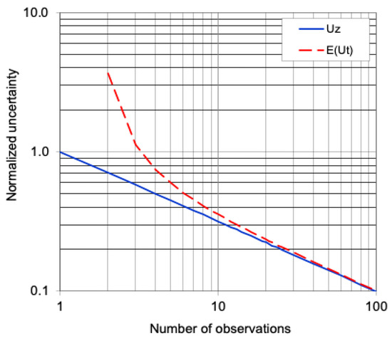
Figure 2.
Uz and (normalized by at 1 − α = 0.95) on the log–log scales [60].
It is worth noting that, prior to Student (William Sealy Gosset), the expanded uncertainty (referred to as the “probable error” in Student’s 1908 paper) was calculated using the maximum likelihood estimate of the population variance. This approach significantly underestimates the uncertainty when the sample size is small, with relative biases of −43.6%, −20.2%, and −7.7% at n = 2, 4, and 10, respectively. To correct for this underestimation, Student [65] invented the t-distribution. However, the t-based uncertainty Ut, derived from the t-distribution, leads to an overestimation of the uncertainty, as evidenced by the inflation factor. Interestingly, Ziliak and McCloskey [66] remarked that “Student used his t-tables a teensy bit…” and noted that “We have learned recently, by the way, that “Student” himself—William Sealy Gosset—did not rely on Student’s t in his own work”.
5.3. Issues with the t-Distribution
The t-interval and t-based uncertainty are constructed using the t-distribution. Therefore, the methodological issues associated with the t-interval and t-based uncertainty must ultimately be traced back to the t-distribution, or its non-standard version: the scaled and shifted t-distribution (referred to as the location-scale t-distribution in Wikipedia).
First, the t-distribution is subject to what Huang [30] termed the “t-transformation distortion”. The t-statistic is computed as the ratio between the sample error and the standard error of the sample mean, which transforms the original ε-s space Ω(ε, s) into a distorted t-space Ω(t). The t-transformation itself is mathematically valid, and thus the t-distribution is also mathematically sound. However, the inferences made using the t-distribution (such as constructing t-intervals) may not be valid because the inferences are actually performed in the distorted t-space Ω(t) [64]. To illustrate, consider that plums are dried to make prunes. The drying process alters the shape and characteristics of the plums, which is analogous to the “t-transformation distortion”. Just as one cannot accurately infer the original shape of plums from the dried prunes, we cannot reliably infer the true properties of the original data from inferences made in the distorted t-space Ω(t).
Second, the scaled and shifted t-distribution is not an appropriate sampling distribution for the sample mean of n observations. According to the Central Limit Theorem, the sampling distribution for the sample mean approximates the normal distribution (or the scaled and shifted z-distribution), regardless of the original distribution. The Central Limit Theorem does not support using the scaled and shifted t-distribution. Moreover, among three candidate distributions, the scaled and shifted t-distribution, the scaled and shifted z-distribution, and the Laplace distribution, Huang [67] demonstrated that the scaled and shifted z-distribution is the best choice according to the minimum entropy criterion, while Huang [68] demonstrated that it is also the best according to the maximum informity criterion. The informity metric is the counterpart of the entropy metric; it can be used as an alternative measure to assess distributions [68]. In summary, the Central Limit Theorem, the entropy metric, and the informity metric all support the use of the scaled and shifted z-distribution instead of the scaled and shifted t-distribution. There is no mathematical or physical principle that justifies the use of the t-distribution or its scaled and shifted version for this purpose.
It is worth mentioning that the statistics textbook by Matloff [69] does not even cover the t-distribution and t-intervals. In fact, Matloff [70] stated the following: “I advocate skipping the t-distribution, and going directly to inference based on the Central Limit Theorem”. This perspective further emphasizes the argument that inference should be based on the more robust and intuitive foundation provided by the Central Limit Theorem, rather than relying on the t-distribution.
6. Alternative to the t-Interval Method for Calculating Measurement Uncertainty: Unbiased Estimation Method
6.1. Unbiased Estimation Method
Again, for a measurement with a small number of observations, when σ is known, the z-based uncertainty Uz is the true expanded uncertainty. In practice, σ may be known from the manufacturer’s precision specification for a measuring instrument. Thus, Uz can be regarded as the true precision. When σ is unknown, however, the true precision cannot be determined. In such cases, the purpose of uncertainty analysis is to estimate the true precision based on the available sample data. According to the theory of point estimation, when σ is unknown, it can be replaced by a sample-based estimator . Accordingly, Uz can be replaced by a sample-based estimator . We want to equal Uz on average, meaning that should be an unbiased estimator of Uz. Note that is an unbiased estimator of σ. Thus, is an unbiased estimator of Uz. This unbiased estimator conforms to the −1/2 power law.
Hirschauer [71] stated the following:
“What we can extract—at best—from a random sample is an unbiased point estimate (signal) of an unknown population effect size and an unbiased estimation of the uncertainty (noise), caused by random error, of that point estimation, i.e., the standard error, which is but another label for the standard deviation of the sampling distribution”.
Indeed, the sample mean (effect size) and the unbiased standard error are “what we can extract—at best—from a random sample…”
The unbiased estimation method can provide realistic uncertainty estimates. The “uncertainty paradox” caused by the t-interval method disappears when using the unbiased estimation method. For the “carpenter’s laugh” scenario described by D’Agostini [33] (mentioned in the Introduction), the t-score at the nominal coverage probability (1 − α) = 0.999 is 636.62 due to severe t-transformation distortion at n = 2, leading to the absurd uncertainty estimate = 95 mm. In contrast, the z-score at (1 − α) = 0.999 is 3.29 and the bias correction factor c4,n at n = 2 is 0.7979. The unbiased estimation method gives = 0.62 mm, which is far more realistic. Moreover, unlike the t-based uncertainty , which is unsuitable for measurement quality control due to its high false rejection rate, the unbiased estimator can be reliably used for measurement quality control. Importantly, this unbiased estimation method has been adopted in the ISO standard for streamflow measurements with acoustic Doppler current profiler [72].
It is important to point out that the unbiased estimation method is applicable to both small and large samples (or small and large degrees of freedom). Therefore, unlike traditional methods that require different approaches depending on the sample size or degrees of freedom, the unbiased estimation method provides a consistent solution regardless of sample size. This is an important advantage.
It should be emphasized that the unbiased estimation method is based on the theory of point estimation and the unbiasedness criterion. Unlike the t-interval method, which is an interval procedure based on confidence interval theory and the “coverage” criterion, the unbiased estimation method is not designed to generate intervals that capture the true value at a specified long-term success rate. These two approaches are mutually incompatible and incommensurable. Therefore, the “coverage” criterion should not be applied to the unbiased estimation method. In other words, the performance of the unbiased estimation method should not be judged by the long-term success or capture rate that is commonly used to evaluate confidence interval procedures [64,73].
Statistics textbooks often claim that interval estimation is more informative than point estimation. However, this claim can be misleading. Suppose we employ a statistical distribution model (e.g., normal distribution) in our analysis. If the model parameters are obtained by a valid method (such as maximum likelihood) applied to a given dataset, we can derive an estimated distribution. This estimated distribution, in turn, enables us to construct any probability interval we desire. For example, with n observations, the sample mean and the unbiased standard error serve as estimates of the location and scale parameters, respectively. Then, the estimated sampling distribution of the sample mean is [74]. This complete estimated distribution is inherently more informative than any single confidence interval constructed from it, as it provides a full probabilistic description of the uncertainty surrounding the parameter estimate rather than a mere interval estimate.
The unbiased estimation method has been extended to cases involving multiple uncertainty components in measurement uncertainty analysis. This extension is referred to as the WS-z approach [35]. The WS-z approach resolves the Ballico paradox that arises from the WS-t approach (mentioned in the Introduction), by providing more realistic and consistent uncertainty estimates.
6.2. Example: A Comparison of the WS-z and WS-t Approaches
Consider two random variables X and Y. We assume that X is normally distributed with an unknown mean and unknown variance, and Y is normally distributed with a mean of 0 and variance of σY. We have n observations from X: {x1, x2, …, xn} and one observation from Y: {y}. Then, is the estimator for Z = X + Y, and the variance of Z is given by
where is the sample standard deviation of the n observations {x1, x2, …, xn}.
Our job is to estimate the expanded uncertainty of the estimate . According to the unbiased estimation method (i.e., the WS-z approach), the expanded uncertainty is given by
where is the bias correction factor and is the effective degrees of freedom (DOF). The effective DOF can be calculated using the Welch–Satterthwaite (WS) formula. For the problem considered, the Welch–Satterthwaite formula can be written as [35]
The expanded uncertainty given by the WS-t approach is [35]
To obtain numerical results for comparison, we assume that , n = 4, and = 0.05, while σY varies from 0 to 3. Under these assumptions, Figure 3 shows the expanded uncertainty estimates produced by the WS-z and WS-t approaches.
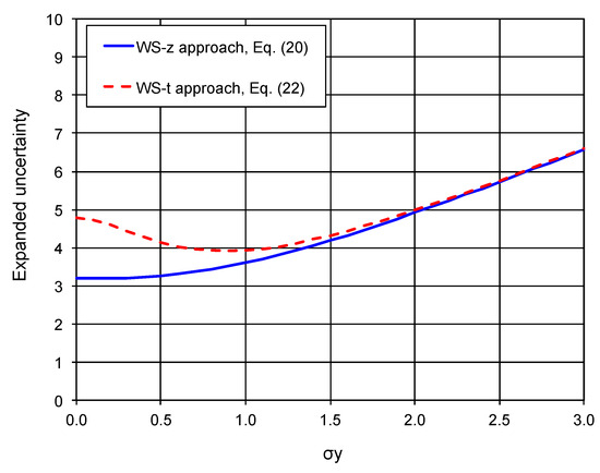
Figure 3.
Expanded uncertainty estimated by the WS-z and WS-t approaches (, n = 4, and = 0.05).
It can be seen from Figure 2 that the WS-z approach gives realistic estimates of the expanded uncertainty. Importantly, the expanded uncertainty increases continuously as σY increases, which conforms with our domain knowledge and common sense regarding measurement uncertainty. In contrast, the WS-t approach provides unrealistic estimates. It not only overestimates uncertainty when σY is small (inflates the uncertainty), but it also exhibits paradoxical behavior: the uncertainty decreases as σY increases in the range from 0 to 0.9. Notably, the WS-t uncertainty estimate converges to the WS-z estimate only when σY becomes large. This is expected because, when σY is large, the contribution from σY dominates over . This example clearly demonstrates that the WS-t approach, or the t-interval method for calculating measurement uncertainty, is inherently flawed.
7. Conclusions and Recommendations
According to Jaynes ([75], p. 758), a paradox is “something which is absurd or logically contradictory, but which appears at first glance to be the result of sound reasoning”. He further explained that “A paradox is simply an error out of control: i.e., one that has trapped so many unwary minds that it has gone public, become institutionalized in our literature, and taught as truth”. In this regard, the two-sample t-test and the t-interval represent such paradoxes. Statistics textbooks, journals, and software packages have played a significant role in disseminating these paradoxical methods. As Hurlbert et al. [76] pointed out, “Many controversies in statistics are due primarily or solely to poor quality control in journals, bad statistical textbooks, bad teaching, unclear writing, and lack of knowledge of the historical literature”.
Therefore, to implement statistics reform, statistics textbooks and software packages should be updated to reflect the paradigm shift from significance testing to estimation statistics. The author agrees with Hurlbert et al. [76], who argued that “… the term ‘statistically significant’ and all its cognates and symbolic adjuncts be disallowed in the scientific literature except where focus is on the history of statistics and its philosophies and methodologies”. Specifically, the two-sample t-test and the t-interval method for calculating measurement uncertainty (both of which are problematic statistical methods) should be removed from textbooks and software packages. In contrast, good statistical methods, such as the least squares method and maximum likelihood estimation, should withstand statistics reform.
The advanced estimation statistics framework should be used in place of the two-sample t-test for comparing two groups. This approach involves considering multiple statistics, including the observed effect size (ES), relative effect size (RES), standard uncertainty (SU), relative standard uncertainty (RSU), signal-to-noise ratio (SNR), signal content index (SCI), exceedance probability (EP), and net superiority probability (NSP), which collectively extract and reveal the evidence embedded in the data from various perspectives. Scientific inferences should be made based on domain knowledge while considering the comprehensive information provided by these statistics.
The unbiased estimation method should be used in place of the t-interval method for calculating measurement uncertainty. When employing the unbiased estimation method, both the “uncertainty paradox” and the Ballico paradox (both inherent to the t-interval method) disappear, leading to more realistic and reliable uncertainty estimates.
The author believes that the success of statistics reform depends on collaboration between statisticians and practitioners. It is hoped that this paper will stimulate discussion on statistics reform and encourage joint efforts to improve statistical practices.
Funding
This research received no external funding.
Data Availability Statement
Data are contained within this article.
Acknowledgments
The author would like to thank the three anonymous reviewers for their valuable comments that helped to improve the quality of this article.
Conflicts of Interest
The author declares no conflicts of interest.
References
- Nuzzo, R. Scientific method: Statistical errors. Nature 2014, 506, 150–152. [Google Scholar] [CrossRef] [PubMed]
- Hirschauer, N.; Grüner, S.; Mußhoff, O. The p-Value and Statistical Significance Testing. In Fundamentals of Statistical Inference; SpringerBriefs in Applied Statistics and Econometrics; Springer: Cham, Switzerland, 2022. [Google Scholar] [CrossRef]
- Siegfried, T. Odds Are, It’s wrong: Science fails to face the shortcomings of statistics. Sci. News 2010, 177, 26. Available online: https://www.sciencenews.org/article/odds-are-its-wrong (accessed on 10 May 2023). [CrossRef]
- Siegfried, T. To Make Science Better, Watch Out for Statistical Flaws. Science News Context Blog, 7 February 2014. Available online: https://www.sciencenews.org/blog/context/make-science-better-watch-out-statistical-flaws (accessed on 10 May 2023).
- Amrhein, V.; Greenland, S.; McShane, B. Retire statistical significance. Nature 2019, 567, 305–307. [Google Scholar] [CrossRef] [PubMed]
- Halsey, L.G. The reign of the p-value is over: What alternative analyses could we employ to fill the power vacuum? Biol. Lett. 2019, 15, 20190174. [Google Scholar] [CrossRef]
- McShane, B.B.; Gal, D.; Gelman, A.; Robert, C.P.; Tackett, J.L. Abandon statistical significance. Am. Stat. 2018, 73, 235–245. [Google Scholar] [CrossRef]
- Wasserstein, R.L.; Lazar, N.A. The ASA’s statement on p-values: Context, process, and purpose. Am. Stat. 2016, 70, 129–133. [Google Scholar] [CrossRef]
- Wasserstein, R.L.; Schirm, A.L.; Lazar, N.A. Moving to a world beyond “p <0.05”. Am. Stat. 2019, 73 (Suppl. S1), 1–19. [Google Scholar] [CrossRef]
- Trafimow, D.; Marks, M. Editorial. Basic Appl. Soc. Psychol. 2015, 37, 1–2. [Google Scholar] [CrossRef]
- Colling, L.J.; Szűcs, D. Statistical Inference and the Replication Crisis. Rev. Philos. Psychol. 2021, 12, 121–147. [Google Scholar] [CrossRef]
- Haig, B.D. Tests of statistical significance made sound. Educ. Psychol. Meas. 2016, 77, 489–506. [Google Scholar] [CrossRef]
- Wagenmakers, E.J.; Wetzels, R.; Borsboom, D.; Van Der Maas, H.L. Why psychologists must change the way they analyze their data: The case of psi: Comment on Bem. J. Personal. Soc. Psychol. 2011, 100, 426–432. [Google Scholar] [CrossRef] [PubMed]
- Amrhein, V.; Greenland, S. Remove, rather than redefine, statistical significance. Nat. Hum. Behav. 2018, 2, 4. [Google Scholar] [CrossRef] [PubMed]
- Cumming, G. The new statistics: Why and how. Psychol. Sci. 2014, 25, 7–29. [Google Scholar] [CrossRef] [PubMed]
- Cumming, G.; Calin-Jageman, R. Introduction to the New Statistics Estimation, Open Science, and Beyond, 2nd ed.; Routledge: Oxfordshire, UK, 2024; ISBN 9780367531508. [Google Scholar]
- Normile, C.J.; Bloesch, E.K.; Davoli, C.C.; Scherr, K.C. Introducing the new statistics in the classroom. Scholarsh. Teach. Learn. Psychol. 2019, 5, 162–168. [Google Scholar] [CrossRef]
- Claridge-Chang, A.; Assam, P. Estimation statistics should replace significance testing. Nat. Methods 2016, 13, 108–109. [Google Scholar] [CrossRef]
- Elkins, M.R.; Pinto, R.Z.; Verhagen, A.; Grygorowicz, M.; Söderlund, A.; Guemann, M.; Gómez-Conesa, A.; Blanton, S.; Brismée, J.M.; Ardern, C.; et al. Statistical inference through estimation: Recommendations from the International Society of Physiotherapy Journal Editors. Eur. J. Physiother. 2022, 24, 129–133. [Google Scholar] [CrossRef]
- Trafimow, D.; Hyman, M.R.; Kostyk, A.; Wang, Z.; Tong, T.; Wang, T.; Wang, C. Gain-probability diagrams in consumer research. Int. J. Mark. Res. 2022, 64, 470–483. [Google Scholar] [CrossRef]
- Trafimow, D.; Tong, T.; Wang, T.; Choy ST, B.; Hu, L.; Chen, X.; Wang, C.; Wang, Z. 2024 Improving Inferential Analyses Pre-Data and Post-Data. Psychol. Methods 2024. to be published. [Google Scholar]
- Benjamini, Y.; De, V.R.; Efron, B.; Evans, S.; Glickman, M.; Graubard, B.I.; He, X.; Meng, X.-L.; Reid, N.; Stigler, S.M.; et al. ASA President’s Task Force Statement on Statistical Significance and Replicability. Harv. Data Sci. Rev. 2021, 3, 10–11. [Google Scholar] [CrossRef]
- Hand, D.J. Trustworthiness of Statistical Inference. J. R. Stat. Soc. Ser. A Stat. Soc. 2022, 185, 329–347. [Google Scholar] [CrossRef]
- Lohse, K. In Defense of Hypothesis Testing: A Response to the Joint Editorial from the International Society of Physiotherapy Journal Editors on Statistical Inference Through Estimation. Phys. Ther. 2022, 102, 118. [Google Scholar] [CrossRef] [PubMed]
- Aurbacher, J.; Bahrs, E.; Banse, M.; Hess, S.; Hirsch, S.; Hüttel, S.; Latacz-Lohmann, U.; Mußhoff, O.; Odening, M.; Teuber, R. Comments on the p-value debate and good statistical practice. Ger. J. Agric. Econ. 2024, 73, 1–3. [Google Scholar] [CrossRef]
- Heckelei, T.; Hüttel, S.; Odening, M.; Rommel, J. The p-value debate and statistical (Mal) practice–implications for the agricultural and food economics community. Ger. J. Agric. Econ. 2023, 72, 47–67. [Google Scholar] [CrossRef]
- Berner, D.; Amrhein, V. Why and how we should join the shift from significance testing to estimation. J. Evol. Biol. 2022, 35, 777–787. [Google Scholar] [CrossRef]
- Joint Committee for Guides in Metrology (JCGM). Evaluation of Measurement Data—Guide to the Expression of Uncertainty in Measurement; GUM 1995 with Minor Corrections; Joint Committee for Guides in Metrology (JCGM): Sevres, France, 2008. [Google Scholar]
- Huang, H. A paradox in measurement uncertainty analysis. In Proceedings of the Measurement Science Conference, Pasadena, CA, USA, 25–26 March 2010. ‘Global Measurement: Economy & Technology’ 1970–2010 Proceedings (DVD). [Google Scholar]
- Huang, H. Uncertainty estimation with a small number of measurements, Part I: New insights on the t-interval method and its limitations. Meas. Sci. Technol. 2018, 29, 015004. [Google Scholar] [CrossRef]
- Huang, H. Uncertainty-based measurement quality control. Accredit. Qual. Assur. 2014, 19, 65–73. [Google Scholar] [CrossRef]
- Jenkins, J.D. The Student’s t-distribution uncovered. In Proceedings of the Measurement Science Conference, Johannesburg, South Africa, 19–21 November 2007. [Google Scholar]
- D’Agostini, G. Jeffeys priors versus experienced physicist priors: Arguments against objective Bayesian theory. In Proceedings of the 6th Valencia International Meeting on Bayesian Statistics, Alcossebre, Spain, 30 May–4 June 1998. [Google Scholar]
- Ballico, M. Limitations of the Welch-Satterthwaite approximation for measurement uncertainty calculations. Metrologia 2000, 37, 61–64. [Google Scholar] [CrossRef]
- Huang, H. On the Welch-Satterthwaite formula for uncertainty estimation: A paradox and its resolution. Cal Lab Int. J. Metrol. 2016, 23, 20–28. [Google Scholar]
- Ziliak, S.T.; McCloskey, D.N. The Cult of Statistical Significance: How the Standard Error Costs Us Jobs, Justice, and Lives; University of Michigan Press: Ann Arbor, MI, USA, 2008. [Google Scholar] [CrossRef]
- Trafimow, D. The Story of My Journey Away from Significance Testing. In A World Scientific Encyclopedia of Business Storytelling; World Scientific: Singapore, 2023; pp. 95–127. [Google Scholar] [CrossRef]
- Fisher, R.A. Statistical Methods and Scientific Inference; Oliver and Boyd: Edinbrgh, UK, 1956. [Google Scholar]
- Huang, H. Exceedance probability analysis: A practical and effective alternative to t-tests. J. Probab. Stat. Sci. 2022, 20, 80–97. [Google Scholar] [CrossRef]
- Halsey, L.G.; Curran-Everett, D.; Vowler, S.L.; Drummond, G.B. The fickle P value generates irreproducible results. Nat. Methods 2015, 12, 179–185. [Google Scholar] [CrossRef]
- Hirschauer, N.; Grüner, S.; Mußhoff, O.; Becker, C. Pitfalls of significance testing and p-value variability: An econometrics perspective. Stat. Surv. 2018, 12, 136–172. [Google Scholar] [CrossRef]
- Lazzeroni, L.C.; Lu, Y.; Belitskaya-Lévy, I. Solutions for quantifying P-value uncertainty and replication power. Nat. Methods 2016, 13, 107–108. [Google Scholar] [CrossRef] [PubMed]
- Bonovas, S.; Piovani, D. On p-Values and Statistical Significance. J. Clin. Med. 2023, 12, 900. [Google Scholar] [CrossRef] [PubMed]
- Stansbury, D. p-Hacking 101: N Chasing. The Clever Machine. 2020. Available online: https://dustinstansbury.github.io/theclevermachine/p-hacking-n-chasing (accessed on 15 July 2024).
- Baguley, T. Standardized or simple effect size: What should be reported? Br. J. Psychol. 2009, 100 Pt 3, 603–617. [Google Scholar] [CrossRef] [PubMed]
- Schäfer, T. On the use and misuse of standardized effect sizes in psychological research. OSF Prepr. 2023, 1–18. [Google Scholar] [CrossRef]
- Huang, H. Signal content index (SCI): A measure of the effectiveness of measurements and an alternative to p-value for comparing two means. Meas. Sci. Technol. 2019, 31, 045008. [Google Scholar] [CrossRef]
- Etz, A. Confidence Intervals? More like Confusion Intervals. The Featured Content Blog of the Psychonomic Society Digital Content Project. 2015. Available online: https://featuredcontent.psychonomic.org/confidence-intervals-more-like-confusion-intervals/ (accessed on 3 March 2023).
- Karlen, D. Credibility of confidence intervals. In Proceedings of the Conference on Advanced Techniques in Particle Physics, Durham, UK, 18–22 March 2002; Whalley, M., Lyons, L., Eds.; 2002; pp. 53–57. [Google Scholar]
- Morey, R.D.; Hoekstra, R.; Rouder, J.N.; Lee, M.D.; Wagenmakers, E.-J. The fallacy of placing confidence in confidence intervals. Psychon. Bull. Rev. 2016, 23, 103–123. [Google Scholar] [CrossRef]
- Morey, R.D.; Hoekstra, R.; Rouder, J.N.; Wagenmakers, E.-J. Continued misinterpretation of confidence intervals: Response to Miller and Ulrich. Psychon. Bull. Rev. 2016, 23, 131–140. [Google Scholar] [CrossRef]
- Trafimow, D. Confidence intervals, precision and confounding. New Ideas Psychol. 2018, 50, 48–53. [Google Scholar] [CrossRef]
- Huang, H. Probability of net superiority for comparing two groups or group means. Lobachevskii J. Math. 2023, 44, 42–54. [Google Scholar] [CrossRef]
- Environment Protection Agency (EPA). Technical Support Document for Water Quality-Based Toxics Control; Office of Water: Washington, DC, USA, 1991; EPA/505/2-90-001.
- Di Toro, D.M. Probability model of stream quality due to runoff. J. Environ. Eng. ASCE 1984, 110, 607–628. [Google Scholar] [CrossRef]
- Huang, H.; Fergen, R.E. Probability-domain simulation—A new probabilistic method for water quality modelling. In Proceedings of the WEF Specialty Conference “Toxic Substances in Water Environments: Assessment and Control”, Cincinnati, OH, USA, 14–17 May 1995. [Google Scholar]
- Krishnamoorthy, K.; Mathew, T.; Ramachandran, G. Upper limits for exceedance probabilities under the one-way random effects model. Ann. Occup. Hyg. 2007, 51, 397–406. [Google Scholar] [CrossRef] [PubMed][Green Version]
- Zaiontz, C. Two Sample t Test: Unequal Variances. Real Statistics Using Excel. 2020. Available online: https://real-statistics.com/students-t-distribution/two-sample-t-test-uequal-variances/ (accessed on 22 August 2023).
- Willink, R. Probability, belief and success rate: Comments on ‘On the meaning of coverage probabilities’. Metrologia 2010, 47, 343–346. [Google Scholar] [CrossRef]
- Huang, H. More on the t-interval method and mean-unbiased estimator for measurement uncertainty estimation. Cal Lab Int. J. Metrol. 2018, 25, 24–33. [Google Scholar]
- Bunge, M. Four concepts of probability. Appl. Math. Model. 1981, 5, 306–312. [Google Scholar] [CrossRef]
- Kempthorne, O. Comments on paper by Dr. E. T. Jaynes ‘Confidence intervals vs Bayesian intervals’. In Foundations of Probability Theory, Statistical Inference, and Statistical Theories and Science; Harper, W.L., Hooker, C.A., Eds.; D. Reidel Publishing Company: Dordrecht, The Netherlands, 1976; Volume II, pp. 175–257. [Google Scholar]
- Huang, H. A unified theory of measurement errors and uncertainties. Meas. Sci. Technol. 2018, 29, 125003. [Google Scholar] [CrossRef]
- Huang, H. Uncertainty estimation with a small number of measurements, Part II: A redefinition of uncertainty and an estimator method. Meas. Sci. Technol. 2018, 29, 015005. [Google Scholar] [CrossRef]
- Student (William Sealy Gosset). The probable error of a mean. Biometrika 1908, VI, 1–25. [Google Scholar]
- Ziliak, S.T.; McCloskey, D.N. Significance redux. J. Socio-Econ. 2004, 33, 665–675. [Google Scholar] [CrossRef]
- Huang, H. A minimum entropy criterion for distribution selection for measurement uncertainty analysis. Meas. Sci. Technol. 2023, 35, 035014. [Google Scholar] [CrossRef]
- Huang, H. The Theory of Informity: A Novel Probability Framework; Bulletin of Taras Shevchenko National University of Kyiv: Kyiv, Ukraine, 2025; accepted for publication. [Google Scholar]
- Matloff, N. Open Textbook: From Algorithms to Z-Scores: Probabilistic and Statistical Modeling in Computer Science; University of California: Davis, CA, USA, 2014. [Google Scholar]
- Matloff, N. Why Are We Still Teaching t-Tests? On the Blog: Mad (Data) Scientist—Data Science, R, Statistic. 2014. Available online: https://matloff.wordpress.com/2014/09/15/why-are-we-still-teaching-about-t-tests/ (accessed on 6 June 2022).
- Hirschauer, N. Some thoughts about statistical inference in the 21st century. SocArXiv 2022, 1–12. [Google Scholar] [CrossRef]
- ISO:24578:2021(E); Hydrometry—Acoustic Doppler Profiler—Method and Application for Measurement of Flow in Open Channels from a Moving Boat, First Edition, 2021–2023. International Organization of Standards (ISO): Geneva, Switzerland, 2021.
- Huang, H. Comparison of three approaches for computing measurement uncertainties. Measurement 2020, 163, 107923. [Google Scholar] [CrossRef]
- Huang, H. Why the scaled and shifted t-distribution should not be used in the Monte Carlo method for estimating measurement uncertainty? Measurement 2019, 136, 282–288. [Google Scholar] [CrossRef]
- Jaynes, E.T. Probability Theory: The Logic of Science; Cambridge University Press: Cambridge, UK, 2003. [Google Scholar]
- Hurlbert, S.H.; Levine, R.A.; Utts, J. Coup de Grâce for a Tough Old Bull: “Statistically Significant” Expires. Am. Stat. 2019, 73 (Suppl. S1), 352–357. [Google Scholar] [CrossRef]


Disclaimer/Publisher’s Note: The statements, opinions and data contained in all publications are solely those of the individual author(s) and contributor(s) and not of MDPI and/or the editor(s). MDPI and/or the editor(s) disclaim responsibility for any injury to people or property resulting from any ideas, methods, instructions or products referred to in the content. |
© 2025 by the author. Licensee MDPI, Basel, Switzerland. This article is an open access article distributed under the terms and conditions of the Creative Commons Attribution (CC BY) license (https://creativecommons.org/licenses/by/4.0/).