New Decomposition Models for Hourly Direct Normal Irradiance Estimations for Southern Africa

Abstract

This research develops and validates new decomposition models for hourly direct Normal Irradiance (DNI) estimations for Southern African data. Localised models were developed using data collected from the Southern African Universities Radiometric Network (SAURAN). Clustered areas within Southern Africa were identified, and the developed cluster decomposition models highlighted the potential advantages of grouping data based on shared geographical and climatic attributes. This clustering approach could enhance decomposition model performance, particularly when local data are limited or when data are available from multiple nearby stations. Further, a regional Southern African decomposition model, which encompasses a wide spectrum of climatic regions and geographic locations, exhibited notable improvements over the baseline models despite occasional overestimation or underestimation. The results demonstrated improved DNI estimation accuracy compared to the baseline models across all testing and validation datasets. These outcomes suggest that utilising a localised model can significantly enhance DNI estimations for Southern Africa and potentially for developing similar models in diverse geographic regions worldwide. The overall metrics affirm the substantial advancement achieved with the regional model as an accurate decomposition model representing Southern Africa. Two stations were used as a validation study, as an application example where no localised model was available, and the cluster and regional models both outperformed the comparative decomposition models. This study focused on validating the model for hourly DNI in Southern Africa within a range of $K_t$-intervals from 0.175 to 0.875, and the range could be expanded and validated for future studies. Implementing accurate decomposition models in developing countries can accelerate the adoption of renewable energy sources, diminishing reliance on coal and fossil fuels.

1. Introduction

Photovoltaic (PV) systems require accurate modelling and monitoring to ensure their profitability. The amount of irradiance at the site, the global plane-of-array irradiance (GPI), is the foundation of designing, modelling and monitoring PV systems. The GPI comprises the plane-of-array’s (POA) direct beam, ground and diffuse irradiance components. GPI is used to model and monitor PV systems, as this shows the amount of generated solar power, and, therefore, it is one of the most important contributing factors to designing a PV system. The global horizontal irradiance (GHI), direct normal irradiance (DNI), and diffuse horizontal irradiance (DHI) components are required to calculate these irradiance components.

Irradiance components with a transposition model calculate GPI ($G_{POA}$) as

$$G_{POA}=G_{BC}+G_{DC}+G_{RC}.$$

(1)

$G_{BC}$ is the direct beam irradiance, $G_{RC}$ is the ground-reflected irradiance, and $G_{DC}$ is the diffuse irradiance component in the POA on the collector. The GHI, DNI, and DHI components are required to calculate $G_{BC}$, $G_{DC}$ and $G_{RC}$. The sum of the DNI projected onto the horizontal surface using the cosine of the solar zenith angle ${\theta }_Z$ and DHI gives the GHI, as shown in Figure 1 [1]:

$$GHI=DNI·cos{\theta }_Z+DHI.$$

(2)

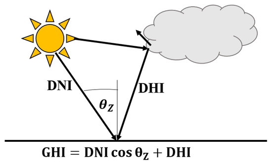
Figure 1. The irradiance relationships between GHI, DNI, DHI, and ${\theta }_Z$.

The units of GHI, DHI, and DNI are $\mathrm{W}/{\mathrm{m}}^2$.

Most ground-based stations at least have measurements of GHI. Other measurements include radiometric data such as DNI, DHI, and ultra-violet and meteorologic data such as the temperature, pressure, rainfall, relative humidity, wind direction and wind speed. Pyranometers measure DHI and GHI, and the pyrheliometer measures DNI.

GHI is measured with a hemispherical view and is mounted horizontally. Similar in setup to other pyranometers, the DHI pyranometer includes the additional feature of being shaded from direct sunlight. The pyrheliometer has a narrow view that only measures the beam directly from the Sun and is usually a Sun tracker for increased accuracy [2]. The irradiance measurements are converted to $\mathrm{W}/{\mathrm{m}}^2$ and logged accordingly.

Calibrating the equipment to the ISO 9060:2018 standard [3] is necessary, and it is advisable to undergo recalibration every two years to ensure the reliability of measurements. The maintenance required is to clean the domes and regularly check and replace the desiccant, which keeps the instruments dry internally.

GHI, DNI, and DHI are interdependent; therefore, having only two irradiance measurements is sufficient to estimate the third using the decomposition models (also sometimes called separation models) [4]. If only the GHI is available, the DNI and DHI also are estimated using the decomposition models. The transposition models calculate GPI using the irradiance components. Therefore, GHI, DHI and DNI correlations are usually empirically expressed as a decomposition model [5].

Indices are relationships between different irradiance components. Decomposition and transposition models utilise these relationships.

The definition of the direct beam transmittance $K_n$ and diffuse transmittance $K_d$ is

$$K_n=\frac{DNI}{G_{0n}},$$

(3)

$$K_d=\frac{DHI}{GHI}.$$

(4)

Ref. [6] defines the $K_t$ as

$$K_t=\frac{GHI}{G_{0n}cos{\theta }_Z}.$$

(5)

All K-values ($K_t$, $K_n$, and $K_d$) are unitless.

The extraterrestrial irradiance on a normal surface $G_{0n}$ depends on the day of the year

$$G_{0n}=\left(\mathrm{Solar}\mathrm{Constant}\right)\left(1+0.033·cos\left(\frac{360·n}{365}\right)\right).$$

(6)

The solar constant is usually 1367 $\mathrm{W}/{\mathrm{m}}^2$.

Determining the horizontal extraterrestrial irradiance $G_{0h}$ involves multiplying it by the cosine of ${\theta }_Z$ as expressed in Equation (7):

$$G_{0h}=G_{0n}·cos{\theta }_Z.$$

(7)

Multipredictor decomposition models can improve accuracy compared to single predictor models [7]. However, the disadvantage is that multiple measurements must be available, which is not always the case for developing countries or brand-new sites of PV installations.

Refs. [8,9] developed a logistical model to estimate solar diffuse radiation [8,9]. Refs. [10,11,12] have proposed machine-learning-based models to predict solar diffusion and direct components [10,11,12]. Ref. [13] proposed a satellite-based decomposition model as an alternative to ground-based measurements [13,14] proposed statistical models for estimating diffuse radiation [14].

Decomposition models have been developed by assessing previous models and improving the accuracy of these estimations. As more data and measurements become available, researchers have the opportunity to develop models for different climates and temporal resolutions. Most models predominantly use $K_t$. Some of the variables used in the decomposition models are the solar altitude angle $\beta$ and dew point temperature $T_d$. Using $K_t$ as the main predictor in decomposition models is popular because of its simplicity and applicability [7].

Ref. [15] developed a relationship between the $K_t$ and $K_d$ [15,16] extended the $K_t$-$K_d$ relationship to latitudes from 31 to 42° North [16]. Ref. [17] established a GHI and DNI relationship for a Mediterranean site to estimate $K_n$ using $K_t$ [17].

The Direct Insolation Simulation Code (DISC) was developed by [18]. Refs. [18,19] developed the Dirint model with the hopes of increasing the performance of the DISC model [19]. The Dirint model of [19] has shown superior performance when estimating the DNI [20].

In Korea, ref. [21] developed a model using six Korean locations. The authors of [4,21] developed a new model using [18]’s DISC model by refitting the coefficients [4]. Ref. [22] developed a DNI estimation model using the solar elevation angle for Norway based on hourly GHI and DHI records [22].

Ref. [23] derived $K_d$ for Hong Kong [23]. Ref. [24] determined $K_d$ using two models with $K_t$ and $\beta$ [24].

The main limitations of decomposition models are that some have a limited climate scope, and the dataset’s temporal resolution affects the irradiance estimation accuracy. A decomposition model in a tropical climate may be unsuitable for a desert climate and vice versa. Intra-hourly-based models perform differently from daily or monthly models, which is why many available decomposition models exist.

The accuracy of decomposition models has been evaluated in several regions, such as Belgium [5], China [25], the USA [20], and North Africa [26].

Ref. [27] provided an extensive study of 140 available decomposition models. The authors state that the predicted DNI’s accuracy highly depends on the decomposition model. Validation studies exist but are limited to a few models and test stations, i.e., biased to a specific location or climate [27]. Research indicates that no decomposition model has been developed and validated for South Africa.

Ref. [28] state that, in general, decomposition models tend to overestimate DHI and underestimate DNI, and typically, models tend to underestimate DHI in overcast periods and overestimate during clear-sky periods [20].

Higher resolution data include higher $K_t$ values, resulting in extreme overestimations of DNI. These hourly DNI estimates have higher accuracy than 1-min DNI estimates. Subhourly estimations would be highly beneficial for the real-time monitoring and forecasting of solar power [27].

Figure 2 visualises the testing and validation countries of common decomposition models in green for models such as [15,16,17,24], DISC ([18]), and Dirint ([4,19,21,22,23]) [4,15,16,17,18,19,21,22,23,24].

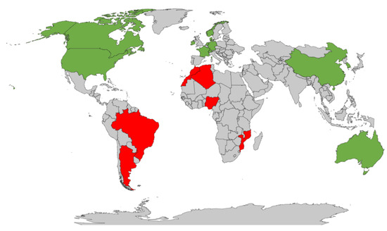
Figure 2. Validation sites of discussed decomposition models.

The decomposition model in South America was developed in Brazil in [29] and in Argentina and Brazil in [30]. Northern African models include Nigeria [31], Algeria [32], and Morocco [33].

Ref. [34] developed a model for Australia and observed that the model only slightly outperformed the Dirint model [34]. The BRL model developed by [9] included a method to construct multiple variable logistic models for the diffuse solar fraction, which includes Mozambique [9]. Figure 2 represents these discussed models [9,29,30,31,32,33,34] in red.

South African research on decomposition models includes the following: ref. [35] published the only Southern African-based study on the relationship between radiation and $K_t$ [35]. However, this relationship is with photosynthetically active radiation related to agricultural practices, not PV systems. Clear-sky model assessments and validation studies have been performed by [36,37] for Southern African countries. Clear-sky models simplify atmospheric attenuation to estimate solar irradiance under clear-sky conditions, do not represent decomposition models, and do not include these studies as comparison models, as they are irrelevant to the research.

Ref. [38]’s thesis assessed decomposition and transposition models in South Africa and showed that the models tend to overestimate the DHI but underestimate the DNI [38]. Furthermore, the DISC and Dirint decomposition models showed the most accurate estimations of the DNI and DHI for South African climatic conditions [39].

As discussed, decomposition models are empirical relationships between GHI, DHI and DNI. All three irradiance components are required to estimate GPI. Decomposition models are useful as they reduce the measurement equipment by decomposing one irradiance component into two others; for example, they use GHI to estimate DHI and DNI.

Most decomposition models are not universally applicable and localised to a specific climate, and the temporal resolution is not always transferable. There has not been extensive literature published representing the Southern African region in decomposition models, which this research article will attempt to address.

2. Model Development

The methodology to develop a novel decomposition model is based on selected data from the automated quality control (QC) procedure proposed in [40] and addresses three geographical models:

• A localised decomposition model, which is site-specific;
• A clustered decomposition model, which encapsulates several sites to group an area based on their geographical location;
• A regional (Southern African) model, which encapsulates the data from the SAURAN network for developing a model specific to Southern Africa.

Figure 3 details an overview of the decomposition model development, which is discussed in this section. The first part is ensuring the data are quality-controlled, followed by the development of the decomposition model. The accuracy of the models are rigorously scrutinised to determine if the proposed models outperform the baseline models.

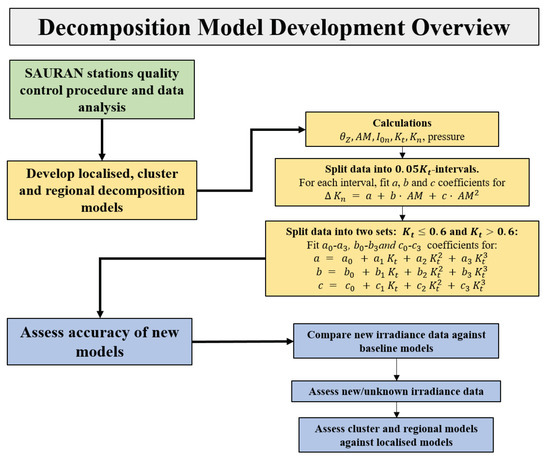
Figure 3. Decomposition model development.

2.1. SAURAN Database

The Southern African Universities Radiometric Network (SAURAN) is a network that includes multiple stations across Southern Africa, collecting meteorological data such as irradiance and wind, among others [41]. Table 1 summarises the SAURAN stations’ corresponding geographical information, such as latitude, longitude, and elevation above sea level.

Table 1. SAURAN station summary [40,41].

	Name (Location)	Coordinates Lat (°S), Long (°E))	Elevation (m)
CSIR	CSIR Energy Centre (Pretoria, South Africa)	25.747, 28.279	1400
CUT	Central University of Technology (Bloemfontein, South Africa)	29.121, 26.216	1397
FRH	University of Fort Hare (Alice, South Africa)	32.785, 26.845	540
GRT	Graaff-Reinet (Graaff-Reinet, South Africa)	32.485, 24.586	660
HLO	Mariendal (Mariendal, South Africa)	33.854, 18.824	178
ILA	Ilanga CSP Plant (Upington, South Africa)	28.490, 21.520	884
KZH	University of KwaZulu-Natal Howard College (Durban, South Africa)	29.871, 30.977	150
KZW	University of KwaZulu-Natal Westville (Durban, South Africa)	29.817, 30.945	200
MIN	CRSES Mintek (Johannesburg, South Africa)	26.089, 27.978	1521
NMU	Nelson Mandela University (Gqeberha, South Africa)	34.009, 25.665	35
NUST	Namibian University of Science and Technology (Windhoek, Namibia)	22.565, 17.075	1683
RVD	Richtersveld (Alexander Bay, South Africa)	28.561, 16.761	141
SUN	Stellenbosch University (Stellenbosch, South Africa)	33.935, 18.867	119
UBG	Gaborone (Gaborone, Botswana)	24.661, 25.934	1014
UFS	University of Free State (Bloemfontein, South Africa)	29.111, 26.185	1491
UNV	Venda (Vuwani, South Africa)	23.131, 30.424	628
UNZ	University of Zululand (KwaDlangezwa, South Africa)	28.853, 31.852	90
UPR	University of Pretoria (Pretoria, South Africa)	25.753, 28.229	1410
VAN	Vanrhynsdorp (Vanrhynsdorp, South Africa)	31.617, 18.738	130

Table 2 summarises the SAURAN database and dataset sizes, followed by Table 3 which shows the subsequent data points available for model development. Further, the data points assessed are $K_t$ between 0.175 and 0.875.

Table 2. SAURAN database and dataset sizes from [41].

Station	Dataset Size		Start Date	End Date
	Before QC	After QC
CSIR	46,434	26,539	11 March 2017	31 October 2022
CUT	28,077	14,619	24 October 2017	31 October 2022
FRH	40,895	22,233	7 February 2017	24 February 2022
GRT	18,541	9774	27 November 2013	24 January 2016
HLO	21,532	11,728	8 October 2015	27 October 2020
ILA	8832	4676	13 October 2021	31 October 2022
KZH	52,323	38,898	7 December 2015	07 August 2022
KZW	20,291	10,756	7 December 2015	12 December 2018
MIN	8185	4423	28 October 2021	31 October 2022
MRB	4201	2462	17 March 2017	22 October 2019
NMU	39,969	23,130	10 December 2015	30 September 2022
NUST	52,004	27,401	26 July 2016	31 October 2022
PMB	9773	5415	13 July 2021	31 October 2022
RVD	63,716	34,457	27 March 2014	28 July 2021
SALT	14,151	9908	21 July 2017	22 December 2020
STA	40,256	21,751	7 December 2015	19 April 2021
SUN	87,720	47,733	24 May 2010	31 October 2022
SUT	1715	902	8 February 2017	20 April 2017
UBG	38,917	20,646	26 November 2014	6 November 2020
UFS	31,665	17,152	16 January 2014	30 August 2017
UNV	59,100	33,144	23 April 2015	31 October 2022
UNZ	56,399	30,373	11 July 2014	31 October 2022
UPR	78,792	42,128	19 September 2013	31 October 2022
VAN	24,701	13,234	26 August 2016	10 July 2019

Table 3. Model development stations indicating the mean GHI, DNI, and GHI and sizes of training, validation, and testing sets.

Station	Mean 1			Dataset 2				Cluster Allocation
	GHI [W/m2]	DNI [W/m2]	DHI [W/m2]	Total	Train	Validation	Test
CSIR	575	599	167	14,991	7495	3748	3748	2
CUT	609	639	159	9161	4580	2290	2291	2
FRH	544	583	151	12,224	6112	3056	3056	4
GRT	573	624	151	5788	2894	1447	1447	4
HLO	550	608	138	7061	3530	1765	1766	1
ILA	589	680	131	2709	0	0	2709	1
KZH	533	517	179	8782	4391	2195	2196	3
KZW	531	511	184	5945	2972	1486	1487	3
NMU	556	545	165	10,562	5281	2640	2641	4
NUST	614	670	149	15,901	7950	3975	3976	1
MIN	564	573	161	2761	0	0	2761	2
RVD	630	729	125	19,624	9812	4906	4906	1
SUN	556	645	133	28,508	14,254	7127	7127	1
UBG	591	602	158	12,137	6068	3034	3035	2
UFS	567	654	137	10,257	5128	2564	2565	2
UNV	579	524	197	15,874	7937	3968	3969	2
UNZ	530	528	176	10,055	5027	2514	2514	3
UPR	568	609	163	28,089	14,044	7022	7023	2
VAN	597	683	126	7860	3930	1965	1965	1

¹ Daylight average, ² Dataset size after quality control as in [40] and 0.175 ≤ K_t ≤ 0.875.

The data points are hourly measurements of the GHI, DNI, and DHI. The split of the train–validation–test datasets is 50:25:25, with the exceptions of two datasets, ILA and MIN. The ILA and MIN have a 0:0:100 data split and are two unknown datasets as part of the test study.

Table 3 also shows each station’s mean GHI, DNI, and DHI, determined after applying the QC procedure.

2.2. Comparison Metrics

The comparison metrics are the root mean square error (RMSE), mean absolute error (MAE), and mean bias error (MBE).

$$\begin{array}{cc}\hfill \mathrm{RMSE}& =\sqrt{\sum _{i=1}^N\frac{{(x_i-\widehat{x_i})}^2}{n}},\hfill \\ \hfill \mathrm{MAE}& =\frac{1}{n}\sum _{i=1}^n|x_i-\widehat{x_i}|,\hfill \\ \hfill \mathrm{MBE}& =\frac{1}{n}\sum _{i=1}^n(x_i-\widehat{x_i}),\hfill \end{array}$$

(8)

where $x_i$ is the measured value and $\widehat{x_i}$ is the predicted value. A low RMSE and MAE indicate a good model, whereas an MBE should be closer to zero. RMSE indicates the concentration of data around the line of best fit. Therefore, a smaller RMSE is indicative of a more accurate model.

The Pearson correlation coefficient r indicates the correlation between data:

$$r=\frac{\sum \left(x_i-\overline{x}\right)\left(y_i-\overline{y}\right)}{\sqrt{\sum {\left(x_i-\overline{x}\right)}^2\sum {\left(y_i-\overline{y}\right)}^2}}.$$

(9)

In Equation (9), $x_i$ and $y_i$ represent the individual points with index i, and $\overline{x}$ and $\overline{y}$ represent the mean of the x and y sample set. An r closer to −1 has a negative correlation, meaning if one variable increases, the other decreases. In contrast, if r is closer to 1, it has a positive correlation, meaning if one variable increases, the other would also [42].

Statistical indicators used for the comparison metrics are the MBE, RMSE, and MAE, which are all expressed as a percentage of the mean measured DNI [27] and $R^2$. Further comparison metrics are two MAE $K_t$-intervals: $K_t<0.60$ and $K_t\ge 0.60$.

The MBE indicates whether a model over- or underestimates the DNI, and the RMSE indicates the deviation of the errors. A significant difference between MAE and RMSE indicates a larger variance in the data. Lower RMSE and MAE are ideal, whereas an MBE closer to zero is optimal. The MAE is an unbiased estimator and also evaluates the two $K_t$ intervals. Lower and higher $K_t$ indicate overcast and clear-sky conditions, respectively. Therefore, the two $K_t$ intervals assess the models under varying weather conditions.

2.3. Regression and Fitting

The relationship between two variables is quantified using statistical methods like regression. Regression techniques can be linear, multi-linear and non-linear.

The definition of a linear relationship is

$$y=b_0+b_{1}x,$$

(10)

where y is the response, x is the regressor, $b_0$ is the intercept, and $b_0$ is the slope. A regression analysis quantifies the strength of a relationship between y and x [42].

The least squares method estimates $b_0$ and $b_1$ so that the sum of the squares of the residuals is at a minimum. The residual sum of squares is denoted as $\mathrm{SSE}$ and is the sum of squares of the errors about the regression line. Thus, the minimisation of

$$\mathrm{SSE}=\sum _{i=1}^n{\left(y_i-\widehat{y_i}\right)}^2,$$

(11)

where $\widehat{y}$ denotes the predicted or fitted value.

The coefficient of determination, $R^2$, indicates how good the fit of a model is and is a number between zero and one.

$$R^2=1-\frac{\sum {\left(y_i-\widehat{y_i}\right)}^2}{{\left(y_i-\overline{y_i}\right)}^2}.$$

(12)

A higher $R^2$ value indicates that the model explains the variation in the response variable around its mean, and the regression model fits the observation better [42].

Polynomial regression is the modelling of a dependent, y, as an $n^{th}$-degree polynomial of x

$$y=b_o+b_{1}x+b_2{x}^2+\cdots +b_r{x}^2.$$

(13)

Exponential regression is where the best fit of an equation is an exponential function, like

$$y=a+b{c}^x,$$

(14)

or

$$y=a+b{e}^{cx}.$$

(15)

Multi-linear regression has multiple variables, which is the outcome of a response variable

$$y={\beta }_0+b_1{x}_{1i}+b_2{x}_{2i}+\cdots +b_k{x}_{ki}.$$

(16)

2.4. Software Development Tools

The model development utilises a combination of data science applications and modelling. The primary tool is the open-source language Python with the anaconda interface [43], and various available libraries [44,45,46].

2.5. Baseline Models

Three comparative models are used as a baseline to compare the new models. Based on the literature, the DISC and Dirint models performed well for Southern African climates [39,47].

The Dirint [19] and Lee [4] models are also used for comparison because their foundation is similar to the DISC model [18].

Ref. [18]’s DISC quasi-physical approach has three assumptions [4]:

• The relative air mass ($AM$) is the dominant parameter affecting the relationship between $K_n$ and $K_t$;
• The physical model used to calculate $K_n$ will provide a physically based reference from which the changes in $K_n$ can be calculated (see Equation (20) below);
• Seasonal, annual and climate variations in the relationship between $K_n$ and $K_t$ are fully accounted for by parametric functions in $K_t$ that relate $\Delta K_n$ to $AM$, cloud cover, and PW vapour.

$AM$ is defined as [48]:

$$AM={\left[cos{\theta }_Z+0.5057·{\left(96.080-{\theta }_Z\right)}^{-1.634}\right]}^{-1}.$$

(17)

The absolute AM ($A{M}_a$) is the pressurised normalisation of AM, expressed as

$$A{M}_a=\mathrm{AM}\left(\frac{P}{P_o}\right),$$

(18)

where P refers to the atmospheric pressure at the test site and $P_o$ is the atmospheric pressure at sea level.

The modelled DNI is determined using Equation (3):

$$DNI=G_{0n}·K_n,$$

(19)

where

$$K_n=K_{nc}-\Delta K_n,$$

(20)

and

$$\Delta K_n=a_{\mathrm{DISC}}+b_{\mathrm{DISC}}{e}^{c_{\mathrm{DISC}}·AM}.$$

(21)

The clear-sky limit $K_{nc}$ is a polynomial in $AM$:

$$\begin{array}{cc}\hfill K_{nc}& =0.866-0.122AM+0.0121A{M}^2-0.00653A{M}^3+0.000014A{M}^4.\hfill \end{array}$$

(22)

Two $K_t$ intervals determine the coefficients $a_{\mathrm{DISC}},b_{\mathrm{DISC}}$ and $c_{\mathrm{DISC}}$: $K_t\le 0.60$ and $K_t>0.60$.

For $K_t\le 0.60$

$$\begin{array}{cc}\hfill a_{\mathrm{DISC}}& =0.512-1.56K_t+2.286K_t^2-2.222K_t^3,\hfill \\ \hfill b_{\mathrm{DISC}}& =0.370+0.962K_t^3,\hfill \\ \hfill c_{\mathrm{DISC}}& =-0.280+0.932K_t-2.048K_t^2.\hfill \end{array}$$

(23)

For $K_t>0.60$

$$\begin{array}{cc}\hfill a_{\mathrm{DISC}}& =-5.743+21.77K_t-27.49K_t^2+11.56K_t^3,\hfill \\ \hfill b_{\mathrm{DISC}}& =41.4-118.5K_t+66.05K_t^2+31.90K_t^3,\hfill \\ \hfill c_{\mathrm{DISC}}& =-47.01+184.2K_t-222.0K_t^2+73.81K_t^3.\hfill \end{array}$$

(24)

Ref. [18]’s model possesses a different functional form because the quasi-physical approach is applied; therefore, it partially reflects the physics involved in the atmospheric transmission of solar radiation [4]. The $a_{\mathrm{DISC}}$, $b_{\mathrm{DISC}}$ and $c_{\mathrm{DISC}}$ parameters were fitted based on solar radiation data from Atlanta, Georgia, USA, 1981 [18]. Ref. [18] adopted the Bird clear-sky model for $K_{nc}$ (see Equation (22)). The parameters $a_{\mathrm{DISC}}$, $b_{\mathrm{DISC}}$ and $c_{\mathrm{DISC}}$, as described in Equations (23) and (24), were then fitted based on the dataset.

The DISC model, termed ‘quasi-physical’, combines a clear-sky model with experimental fits for other sky conditions. The model is a clear-sky irradiance attenuated by a function of $K_t$. The authors of [18] derived the empirical regressions from 12 years of recorded radiation data at 70 stations [5,18].

The Dirint model is based on the DISC model and was developed by [19]. The goal was to improve the accuracy of the DISC model by [18].

The Dirint model uses a clearness index variation parameter $K_t^{\prime }$:

$$K_t^{\prime }=\frac{K_t}{1.031e^{-1.4/(0.9+9.4/AM)}+0.1}.$$

(25)

Furthermore, a stability index parameter $\Delta K_t^{\prime }$,

$$\Delta K_t^{\prime }=0.5\left(|K_{t\left(i\right)}^{\prime }-K_{t(i+1)}^{\prime }|+|K_{t\left(i\right)}^{\prime }-K_{t(i-1)}^{\prime }|\right),$$

(26)

considers the previous ($i-1$), current (i) and next hourly ($i+1$) record. When the preceding or hourly record is missing, $\Delta K_t^{\prime }$ is

$$\Delta K_t^{\prime }=|K_{t\left(i\right)}-K_{t(i\pm 1)}|.$$

(27)

A low $\Delta K_t^{\prime }$ is a stable condition, whereas a high $\Delta K_t^{\prime }$ characterises unstable conditions, which allows the distinction between hazy and partly cloudy conditions. The $T_d$ is an adequate atmospheric PW estimator [19]. The Dirint model’s atmospheric PW (W) is estimated using

$$W=exp(0.07·T_d-0.075).$$

(28)

The Dirint is a four-dimension conditional model, with the ${\theta }_Z$, $K_t$, $\Delta K_t^{\prime }$ and W. Based on the four-dimensional model, the calculation of hourly DNI is

$$DNI=\frac{I_{0n}·k_b^{\prime }{e}^{-1.4/(0.9+9.4/AM)}}{0.87291}.$$

(29)

where

$$\begin{array}{cc}\hfill k_b^{\prime }& =0\mathrm{for}{K}_t^{\prime }<0.2,\hfill \\ \hfill k_b^{\prime }& =a_{\mathrm{Dirint}}{K}_t^{\prime }+b_{\mathrm{Dirint}}.\hfill \end{array}$$

(30)

Coefficients $a_{\mathrm{Dirint}}$ and $b_{\mathrm{Dirint}}$ are from a complex lookup table.

Ref. [4] created a new model for Korea with the same format as [18]’s DISC model.

$$\begin{array}{cc}\hfill a_{\mathrm{Lee}}& =0.342-0.3782K_t,\hfill \\ \hfill b_{\mathrm{Lee}}& =0.5329+0.2676K_t-0.0216k_t^2+0.1584K_t^3.\hfill \end{array}$$

(31)

For $K_t\le 0.5$

$$c_{\mathrm{Lee}}=-0.2117-0.0513K_t+1.2976K_t^2-3.3222K_t^3$$

(32)

or $K_t>0.5$

$$c_{\mathrm{Lee}}=0.7221-10.2801K_t+30.3285K_t^2-27.9766K_t^3.$$

(33)

The evaluation consists of comparing the localised, clustered and regional models against the three baseline models: DISC, Dirint and Lee. The DISC and Dirint models were selected based on their performance in estimating DNI for Southern African climates. The Lee and Dirint models have foundational similarities to the DISC model. These models consider whether the newly developed decomposition model improves the accuracy of hourly DNI estimations for Southern Africa. The accuracy evaluation uses the comparison metrics discussed in the next section.

2.6. Decomposition Model Development Methodology

The methodology builds on the DISC model. The DISC model stands out as one of the better-performing models for estimating DNI for South Africa [39]. Its simplicity is evident in its lack of a need for a complex four-dimensional lookup table, unlike the Dirint model.

The original DISC model uses Equation (21), an exponential function. However, the regression model for an exponential function, as discussed in Section 2.3, showed difficulty in finding optimal a, b and c coefficients in all cases. Instead, a second-order polynomial function of $AM$

$$\Delta K_n=a+b·AM+c·A{M}^2$$

(34)

is a suitable substitute with similar regression results.

The training set then fits a, b and c for intervals $K_t\le 0.60$ and $K_t>0.60$:

$$\begin{array}{cc}\hfill a& =a_0+a_1{K}_t+a_2{K}_t^2+a_3{K}_t^3,\hfill \\ \hfill b& =b_0+b_1{K}_t+b_2{K}_t^2+b_3{K}_t^3,\hfill \\ \hfill c& =c_0+c_1{K}_t+c_2{K}_t^2+c_3{K}_t^3,\hfill \end{array}$$

(35)

and the validation and testing sets evaluate the model’s accuracy.

Figure 3 summarises the development for each decomposition model in this study, where each model undergoes the following initial processing steps:

• Empirical formulae estimate ${\theta }_Z$, $AM$, pressure, $I_{0n}$, $K_t$, and $K_n$. From this, the assessment of available models aids in developing a new model.
• Data are split into intervals of 0.05 $K_t$, starting from 0.175 to 0.875.
• $\Delta K_n$ is then modelled as Equation (34);
• The interval or intervals are then fitted against the function to determine Equation (34) to determine the a, b and c coefficients using a least squares regression analysis.
• From the $K_t$-interval function, the $a_0$-$a_3$, $b_0$-$b_3$ and $c_0$-$c_3$ coefficients are fitted to a polynomial of Equation (35) with regards to $K_t$.
• These equations can be used to determine $\Delta K_n$ and $K_n$, which, in turn, calculate the DNI (see Equations (19) and (20)).

For each SAURAN station, a localised decomposition model is developed. A clustered decomposition model describes an area with similar irradiance patterns using the clustered areas discussed in [40]. Ref. [49] first presented a two-cluster correlation map using the SAURAN database [49], and, by using this approach, this study formulated four clusters instead of two in Southern Africa, as shown in Figure 4a.

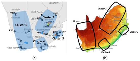
Figure 4. Clusters within the Southern African context. (a) SAURAN [41]; (b) GHI across South Africa [50].

Figure 4a shows the clusters’ geographical location, and Figure 4b shows the penetration levels of GHI. Table 4 shows the different clusters’ training sets’ mean GHI, DNI, and DHI.

Table 4. Mean cluster irradiances.

	Mean 4
	GHI	DNI	DHI
	[$\mathbf{W}/{\mathbf{m}}^{\mathbf{2}}$]	[$\mathbf{W}/{\mathbf{m}}^{\mathbf{2}}$]	[$\mathbf{W}/{\mathbf{m}}^{\mathbf{2}}$]
Cluster 1	592	669	135
Cluster 2	583	604	165
Cluster 3	534	523	178
Cluster 4	557	579	158

⁴ Mean values of training set.

Cluster 1 receives the most GHI and DNI, and Cluster 3 receives the least, as evident from Figure 4b. The different climates are also evident in these clusters: Cluster 3 is more humid and receives, on average, more DHI than Cluster 1.

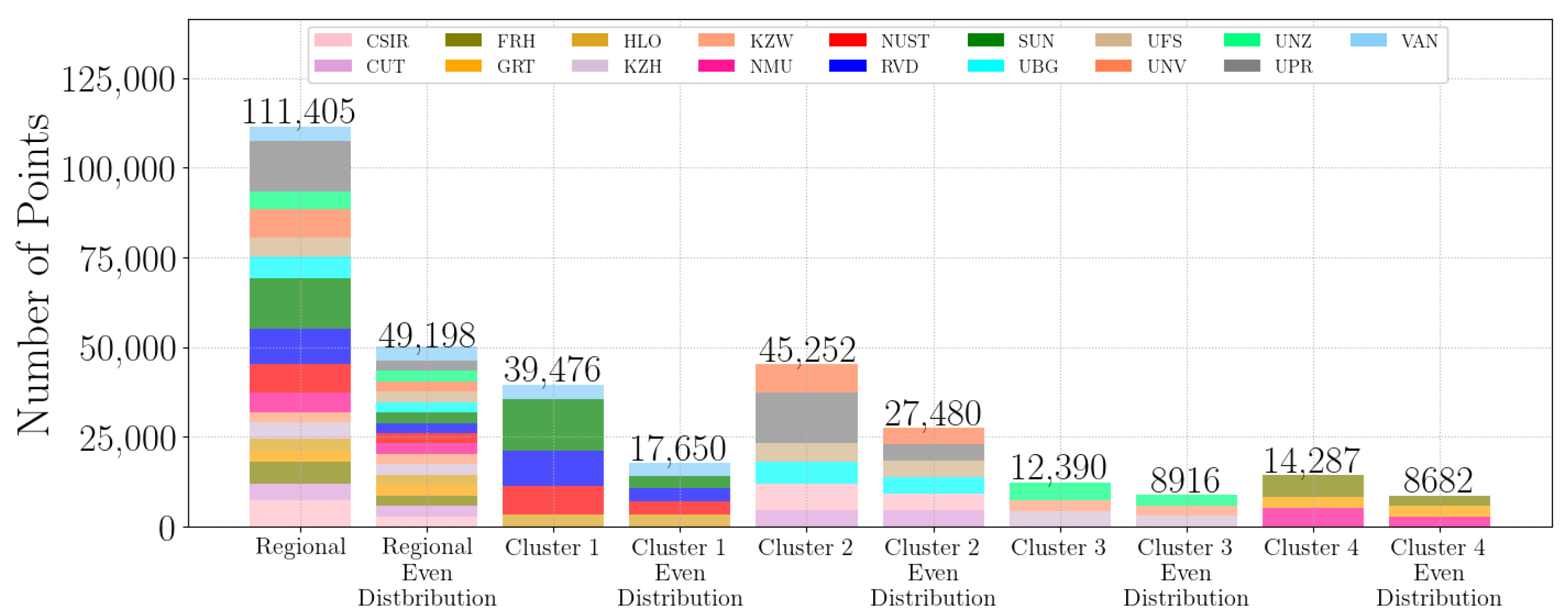
Figure 5 shows how the cluster data are combined. Each cluster and the regional (Southern African) model are combined with even distributions of datasets to avoid introducing a bias, as some stations are over-represented in the original dataset. Some stations, such as the SUN, UPR and RVD stations, have considerably more data available as they are either older stations or have not been closed down.

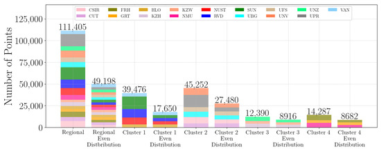
Figure 5. Distribution of data within clusters.

The different stations have varying climates, and therefore, a larger representation of one station will result in a biased model towards that station. The advantage of the even distribution is that every station is sufficiently represented and will not cause a model bias, but this reduces the amount of available data.

Cluster 2’s stations have higher elevation and summer humidity due to its warm, rainy summers and dry, cold winters. The expected annual irradiance levels are lower, as seen in Figure 4b. The stations have higher humidity because of their location and higher DHI levels.

The two stations in Cluster 2, UPR and CSIR, are expected to have more diffuse particles due to the higher air pollution levels and, therefore, higher DHI levels. Cluster 2 has a large bias of the data from Pretoria, South Africa, from the CSIR and UPR datasets.

Cluster 4 has lower annual irradiance levels, as seen in Figure 4b, and FRH and NMU are closer to the coastline, whereas GRT is inland.

3. Development of New Decomposition Models

This section discusses the newly developed a, b and c coefficients of Equation (34).

The section consists of three subsections:

• The localised decomposition models, developed using the training dataset of the SAURAN station;
• The clustered decomposition models, which are modelled on the training data of all the stations within the cluster, as discussed in Figure 5;
• The regional model is modelled on all the stations’ training data (Table 3).

3.1. Localised Decomposition Models

The localised decomposition model equations for the a, b and c coefficients are presented in Appendix A.

3.2. Cluster Decomposition Models

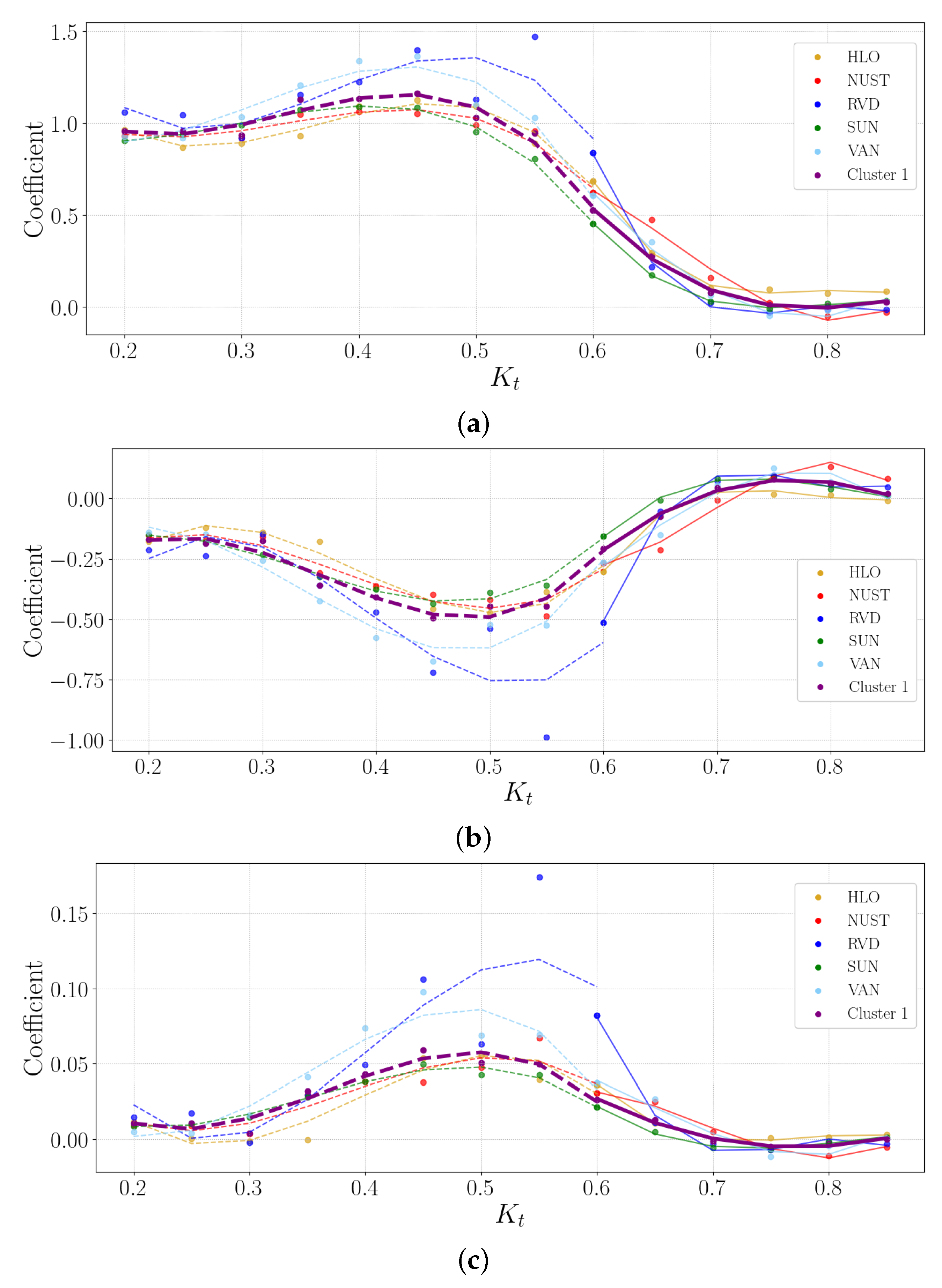
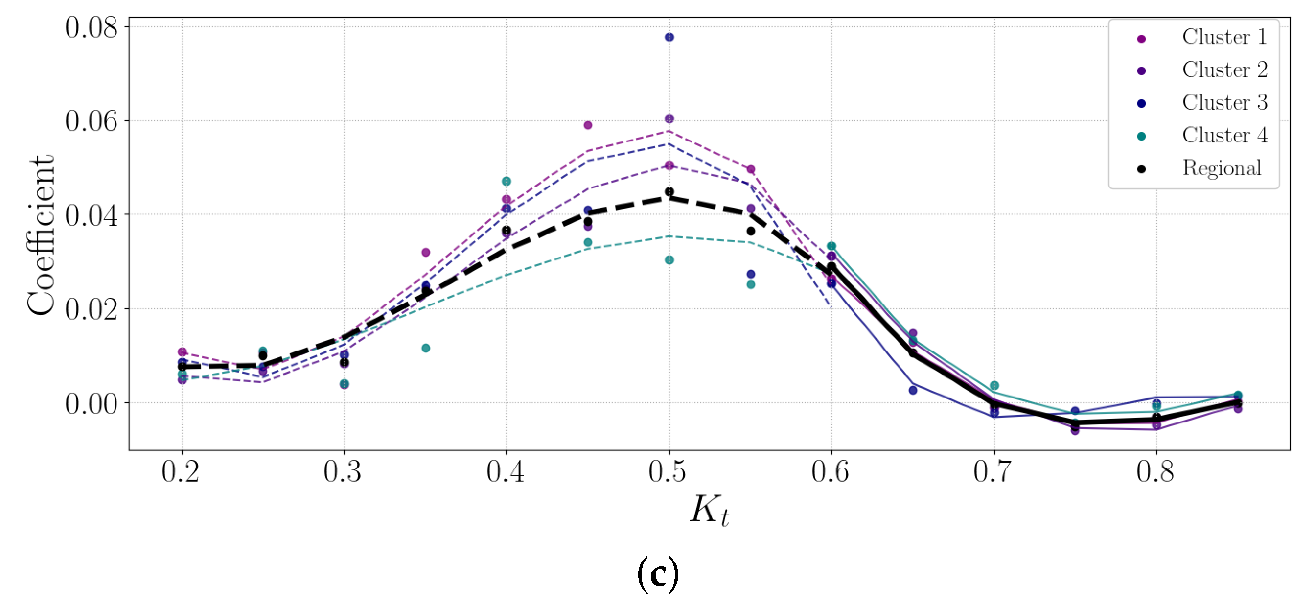
Figure 6, Figure 7, Figure 8 and Figure 9 show the different corresponding clusters’ model coefficients.

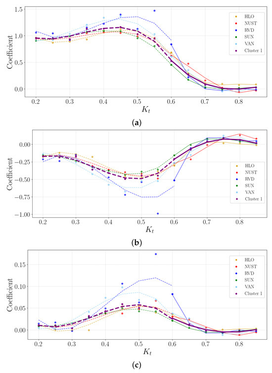
Figure 6. Cluster 1 coefficients in $\Delta K_n=a+b·AM+c·A{M}^2$. (a) a coefficient; (b) b coefficient; (c) c coefficient.

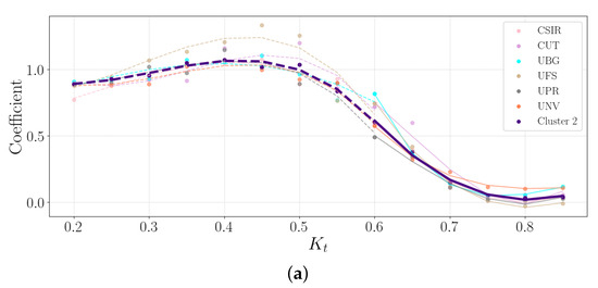
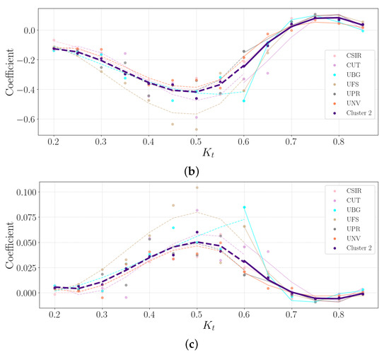
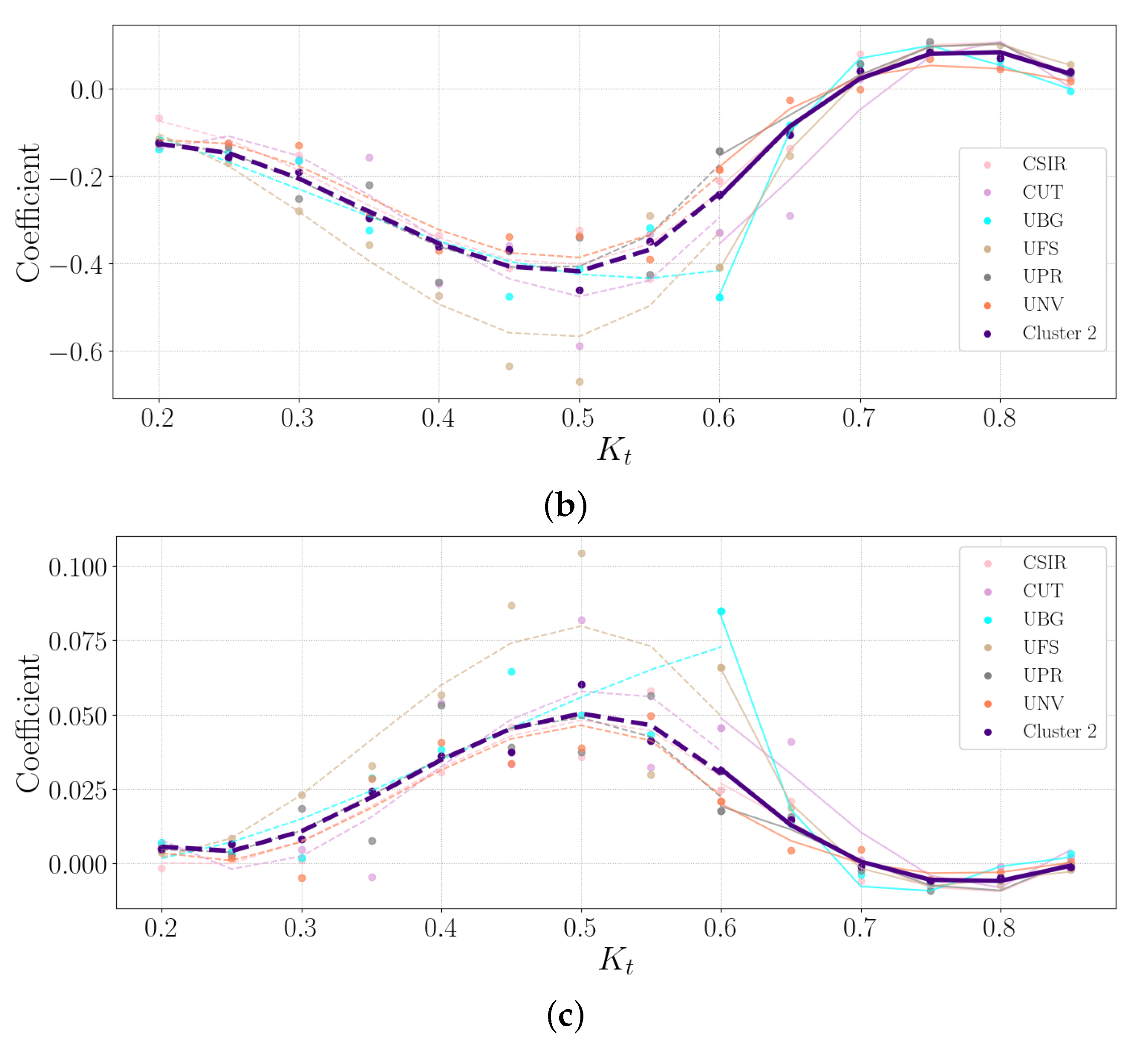
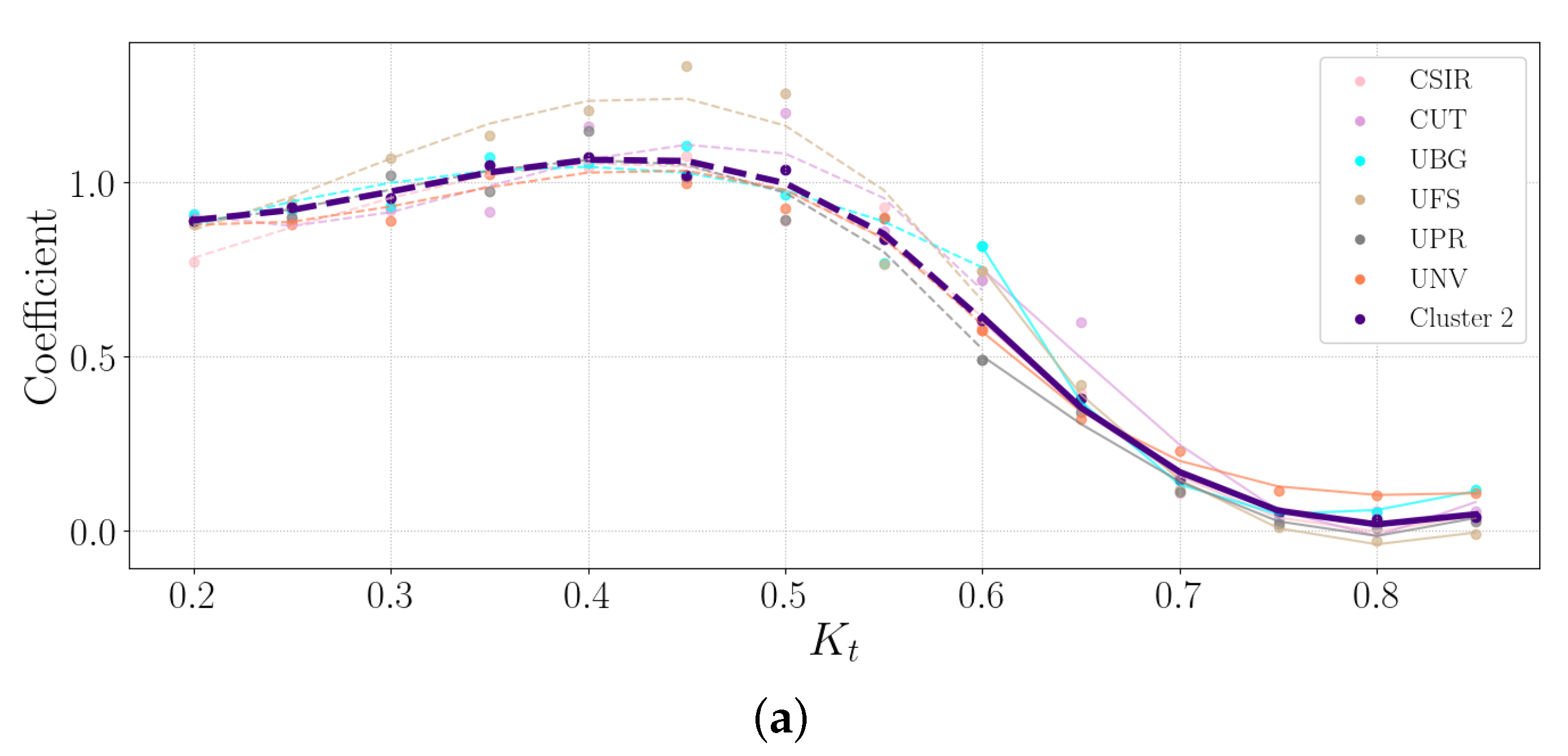
Figure 7. Cluster 2 coefficients in $\Delta K_n=a+b·AM+c·A{M}^2$. (a) a coefficient; (b) b coefficient; (c) c coefficient.

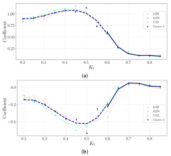
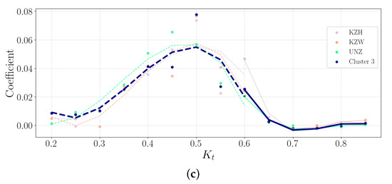
Figure 8. Cluster 3 coefficients in $\Delta K_n=a+b·AM+c·A{M}^2$. (a) a coefficient; (b) b coefficient; (c) c coefficient.

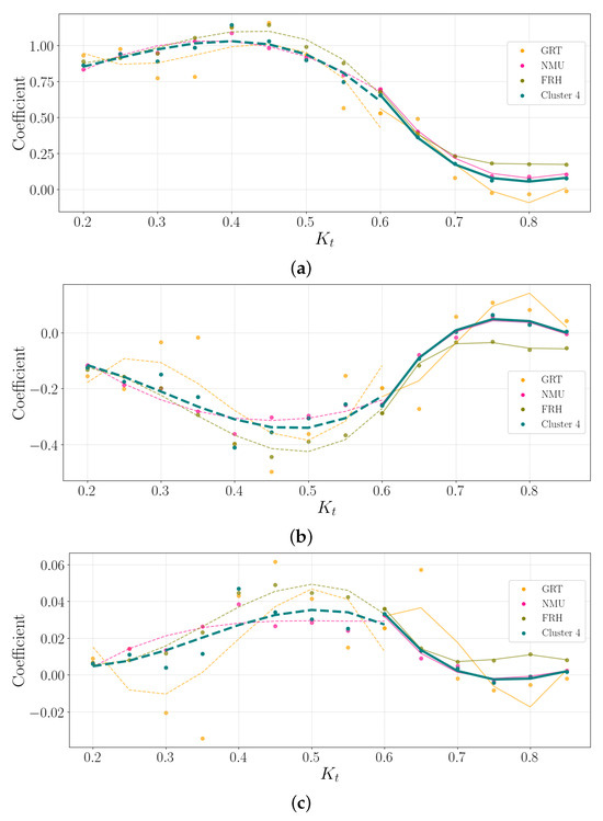
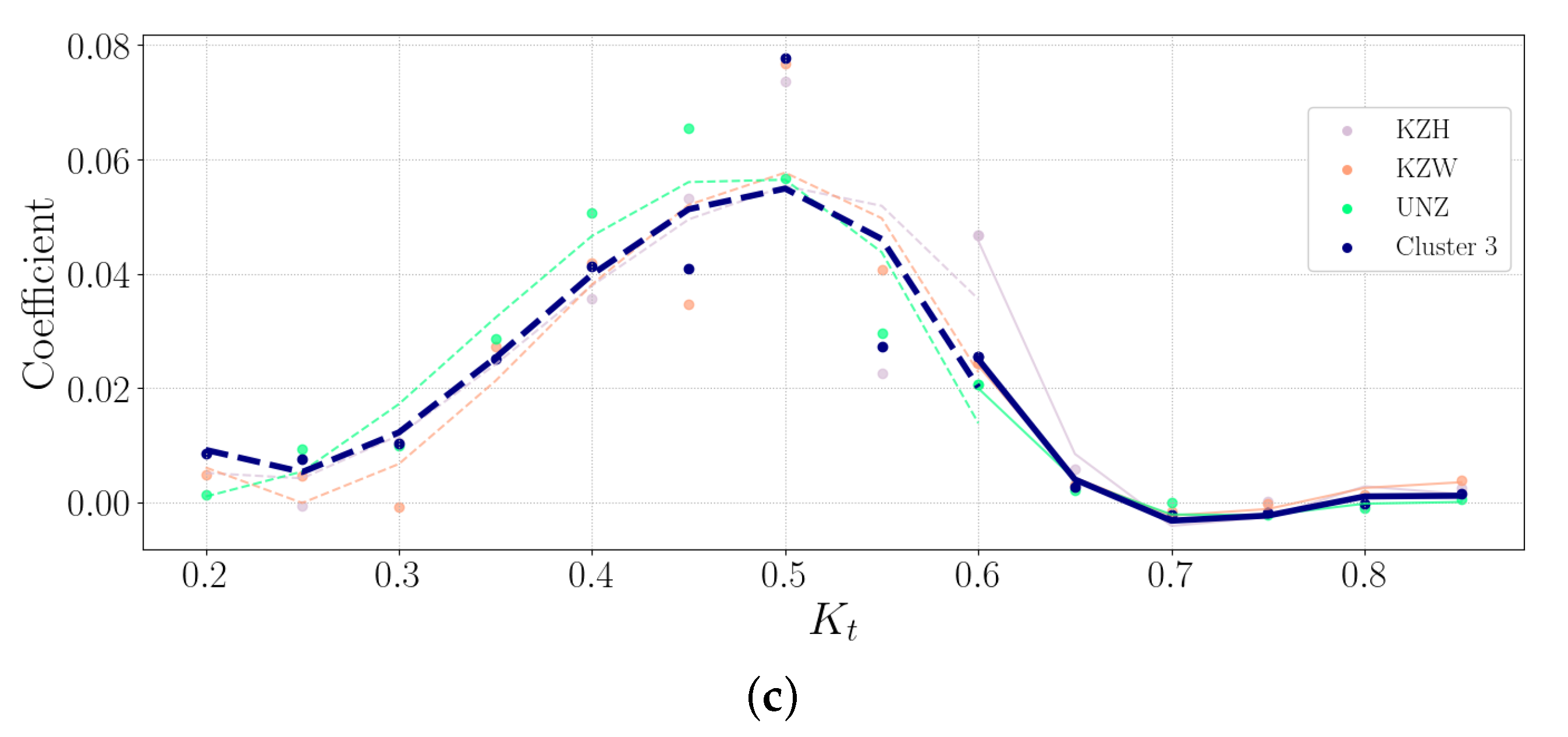
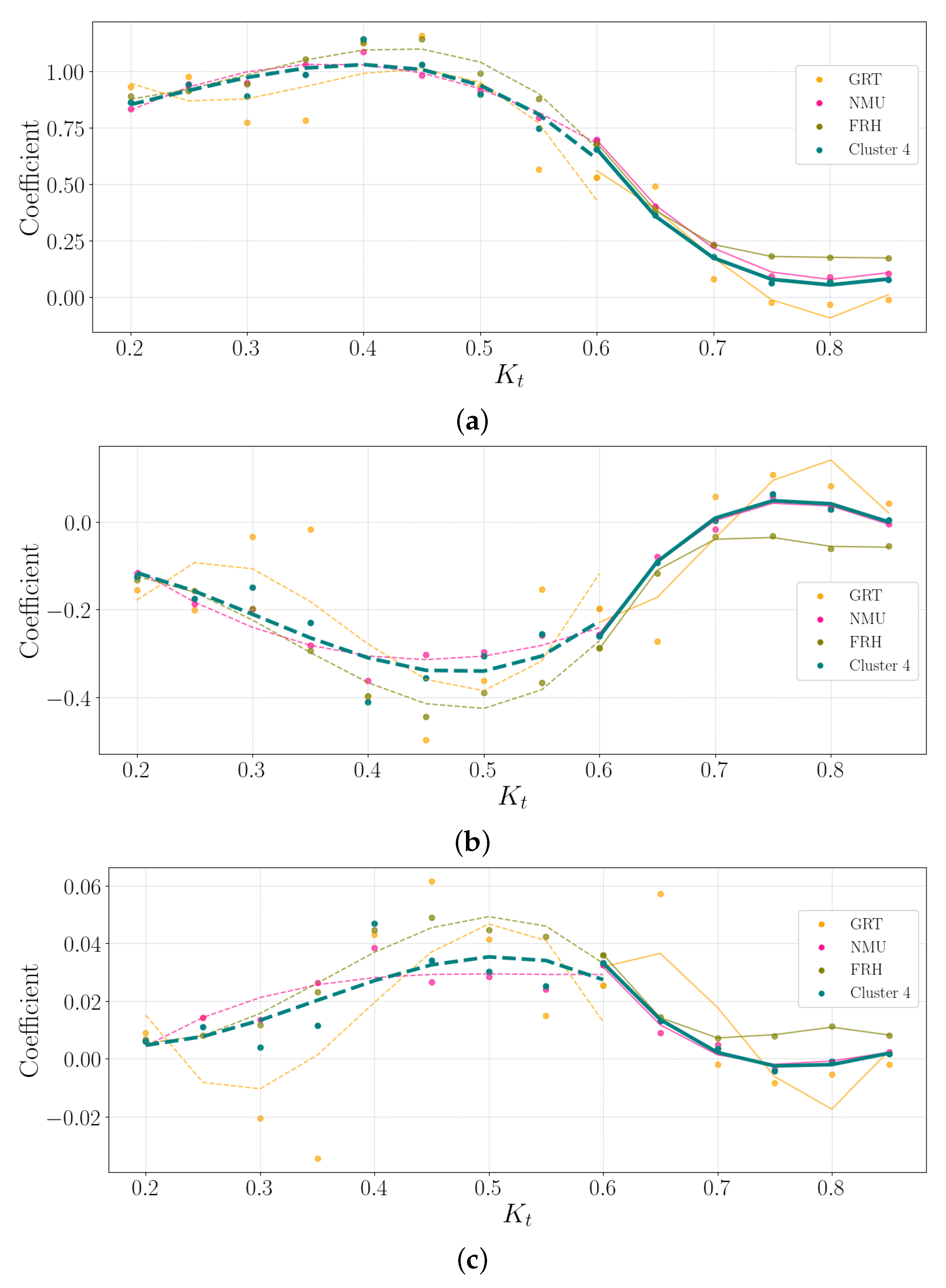
Figure 9. Cluster 4 coefficients in $\Delta K_n=a+b·AM+c·A{M}^2$. (a) a coefficient; (b) b coefficient; (c) c coefficient.

3.2.1. Cluster 1

Cluster 1 comprises the HLO, NUST, RVD, SUN and VAN datasets, as shown in Figure 4a and Figure 5.

Figure 6 shows the Cluster 1 and five stations’ a, b and c coefficients. The discussion of the different stations is in Appendix A under Appendix A.5 (HLO), Appendix A.11 (NUST), Appendix A.12 (RVD), Appendix A.13 (SUN) and Appendix A.19 (VAN).

The RVD model is the only model showing difficulty fitting the coefficients with $K_t$. Table 3 indicates that the RVD station has the highest mean DNI and GHI, with the lowest DHI measurements, compared to the rest of Cluster 1’s stations.

The coefficients for Cluster 1 are

$$\begin{array}{c}\hfill a=\left\{\begin{array}{c}2.4134-15.428K_t+50.7433K_t^2-50.3864K_t^3\mathrm{for}{K}_t<0.60,\hfill \\ 18.4363-61.7241K_t+67.5365K_t^2-23.9963K_t^3\mathrm{for}{K}_t\ge 0.60\hfill \end{array}\right.\\ \hfill b=\left\{\begin{array}{c}-1.4538+13.4628K_t-43.4278K_t^2+40.7081K_t^3\mathrm{for}{K}_t<0.60,\hfill \\ -7.7071+23.0993K_t-20.5561K_t^2+4.7883K_t^3\mathrm{for}{K}_t\ge 0.60\hfill \end{array}\right.\\ \hfill c=\left\{\begin{array}{c}0.2232-2.1593K_t+6.6964K_t^2-6.0805K_t^3\mathrm{for}{K}_t<0.60,\hfill \\ 0.7064-1.9679K_t+1.5214K_t^2-0.2153K_t^3\mathrm{for}{K}_t\ge 0.60\hfill \end{array}\right.\end{array}$$

(36)

3.2.2. Cluster 2

Cluster 2 consists of the CSIR, CUT, UBG, UFS, UPR, and UNV datasets. Figure 7 shows the Cluster 2 and six stations’ a, b and c coefficients.

The discussion of the different stations are in Appendix A under Appendix A.1 (CSIR), Appendix A.2 (CUT), Appendix A.14 (UBG), Appendix A.15 (UFS), Appendix A.18 (UPR) and Appendix A.16 (UNV). The UFS have the greatest deviation from the Cluster 2 fit.

The coefficients for Cluster 2 are

$$\begin{array}{c}\hfill a=\left\{\begin{array}{c}1.4234-6.6647K_t+25.5673K_t^2-27.8939K_t^3\mathrm{for}{K}_t<0.60,\hfill \\ 10.5939-28.4856K_t+21.7611K_t^2-3.348K_t^3\mathrm{for}{K}_t\ge 0.60.\hfill \end{array}\right.\\ \hfill b=\left\{\begin{array}{c}-0.8033+7.723K_t-26.9074K_t^2+25.9995K_t^3\mathrm{for}{K}_t<0.60,\hfill \\ -6.1286+15.6674K_t-9.4832K_t^2-0.4949K_t^3\mathrm{for}{K}_t\ge 0.60.\hfill \end{array}\right.\\ \hfill c=\left\{\begin{array}{c}0.1604-1.5968K_t+5.0219K_t^2-4.537K_t^3\mathrm{for}{K}_t<0.60,\hfill \\ 0.8966-2.6121K_t+2.2392K_t^2-0.4802K_t^3\mathrm{for}{K}_t\ge 0.60.\hfill \end{array}\right.\end{array}$$

(37)

3.2.3. Cluster 3

Cluster 3 consists of the KZH, KZW and UNZ datasets. Figure 8 shows the Cluster 3 and three stations’ a, b and c coefficients.

The discussion of the different stations is in Appendix A under Appendix A.7 (KZH), Appendix A.8 (KZW) and Appendix A.17 (UNZ). The three models fit quite well and are similar to Cluster 3.

The coefficients for Cluster 3 are

$$\begin{array}{c}\hfill a=\left\{\begin{array}{c}1.7678-9.8995K_t+34.9076K_t^2-36.2495K_t^3\mathrm{for}{K}_t<0.60,\hfill \\ 41.1735-157.5062K_t+201.1335K_t^2-85.5391K_t^3\mathrm{for}{K}_t\ge 0.60.\hfill \end{array}\right.\\ \hfill b=\left\{\begin{array}{c}-1.0914+10.2302K_t-33.9924K_t^2+32.4023K_t^3\mathrm{for}{K}_t<0.60,\hfill \\ -31.151+121.964K_t-158.1413K_t^2+67.9737K_t^3\mathrm{for}{K}_t\ge 0.60.\hfill \end{array}\right.\\ \hfill c=\left\{\begin{array}{c}0.2256-2.1961K_t+6.8092K_t^2-6.1997K_t^3\mathrm{for}{K}_t<0.60,\hfill \\ 3.4215-13.4513K_t+17.5277K_t^2-7.5726K_t^3\mathrm{for}{K}_t\ge 0.60.\hfill \end{array}\right.\end{array}$$

(38)

3.2.4. Cluster 4

Cluster 4 consists of the NMU, FRH and GRT datasets. Figure 9 shows the Cluster 4 and three stations’ a, b and c coefficients.

The discussion of the different stations is in Appendix A under Appendix A.10 (NMU), Appendix A.3 (FRH) and Appendix A.4 (GRT). The GRT station’s c-coefficient does show difficulty in a fit determination.

The coefficients for Cluster 4 are

$$\begin{array}{c}\hfill a=\left\{\begin{array}{c}0.7671-0.9387K_t+9.7073K_t^2-14.2827K_t^3\mathrm{for}{K}_t<0.60,\hfill \\ 20.0495-67.0086K_t+73.6919K_t^2-26.4669K_t^3\mathrm{for}{K}_t\ge 0.60.\hfill \end{array}\right.\\ \hfill b=\left\{\begin{array}{c}-0.2382+2.3908K_t-11.3676K_t^2+12.3585K_t^3\mathrm{for}{K}_t<0.60,\hfill \\ -12.5095+42.6536K_t-47.1486K_t^2+16.8022K_t^3\mathrm{for}{K}_t\ge 0.60.\hfill \end{array}\right.\\ \hfill c=\left\{\begin{array}{c}0.0451-0.5012K_t+1.8485K_t^2-1.7706K_t^3\mathrm{for}{K}_t<0.60,\hfill \\ 1.4976-5.1597K_t+5.8075K_t^2-2.1264K_t^3\mathrm{for}{K}_t\ge 0.60.\hfill \end{array}\right.\end{array}$$

(39)

3.3. Regional Decomposition Model

The regional (Southern African) decomposition model data are an even distribution of the SAURAN stations regarding the number of data points used per station. Multiple climates, different elevations, and various pollution levels are represented within the dataset, leading to a better decomposition model for Southern Africa and a regional application.

Figure 10 shows the coefficients a, b and c of the regional model and the four clusters.

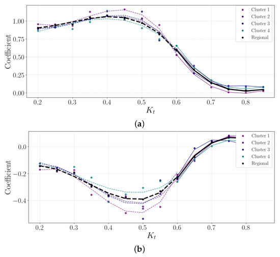
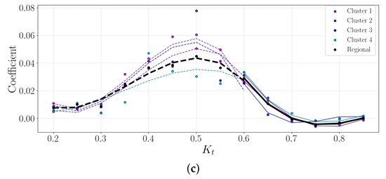
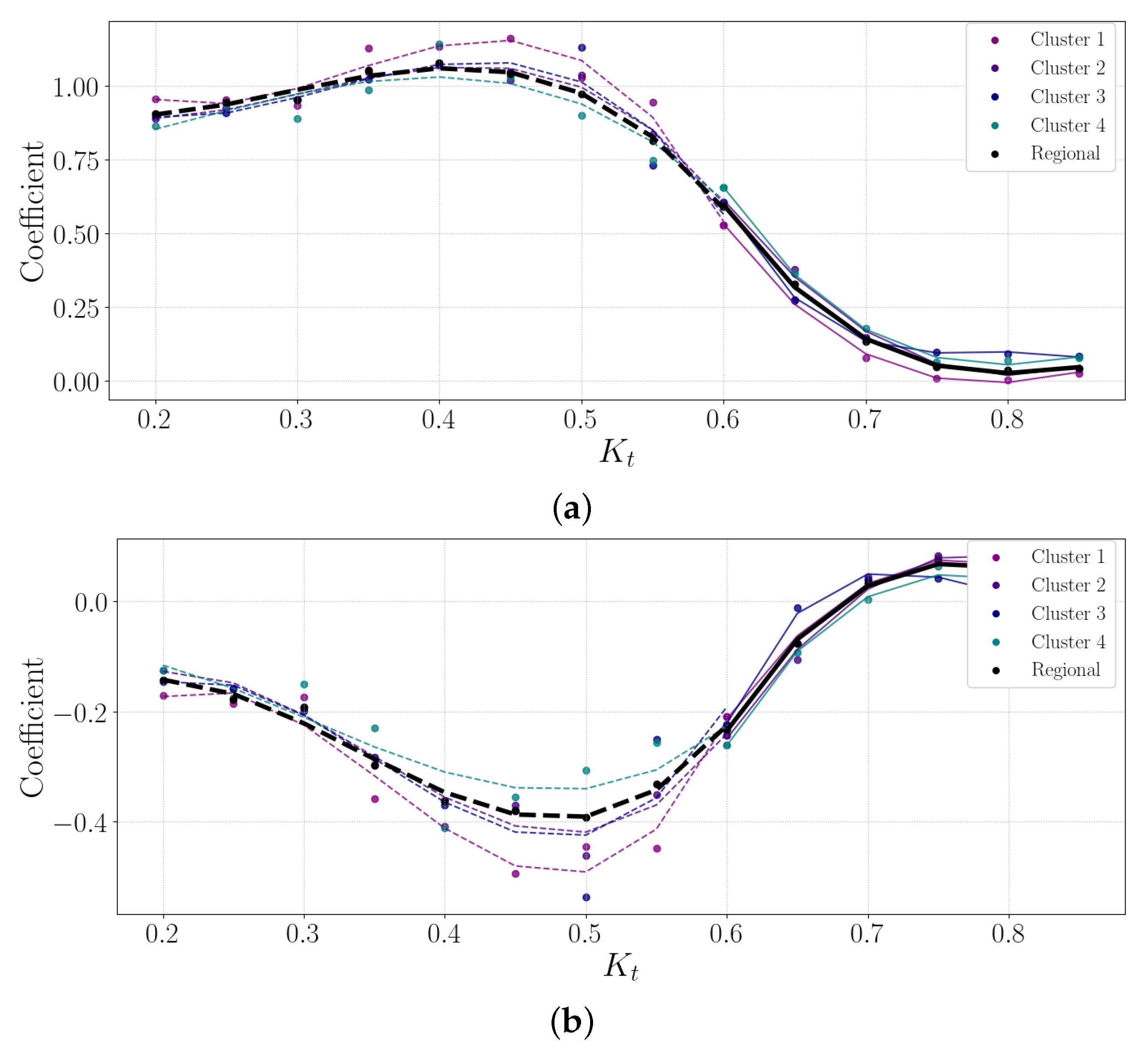
Figure 10. Regional model coefficients in $\Delta K_n=a+b·AM+c·A{M}^2$. (a) a coefficient; (b) b coefficient; (c) c coefficient.

The coefficients for the regional model are

$$\begin{array}{c}\hfill a=\left\{\begin{array}{c}1.2893-5.2531K_t+21.5081K_t^2-24.5156K_t^3\mathrm{for}{K}_t<0.60,\hfill \\ 19.0295-63.9357K_t+70.7485K_t^2-25.6524K_t^3\mathrm{for}{K}_t\ge 0.60.\hfill \end{array}\right.\\ \hfill b=\left\{\begin{array}{c}-0.6327+5.891K_t-21.4431K_t^2+21.2593K_t^3\mathrm{for}{K}_t<0.60,\hfill \\ -11.7813+39.923K_t-43.6596K_t^2+15.3252K_t^3\mathrm{for}{K}_t\ge 0.60.\hfill \end{array}\right.\\ \hfill c=\left\{\begin{array}{c}0.1118-1.1105K_t+3.6089K_t^2-3.3222K_t^3\mathrm{for}{K}_t<0.60,\hfill \\ 1.49-5.2009K_t+5.9381K_t^2-2.2137K_t^3\mathrm{for}{K}_t\ge 0.60.\hfill \end{array}\right.\end{array}$$

(40)

4. Results

Each station is discussed individually by assessing the dataset’s comparison metrics: the $R^2$-value, MBE, RMSE, MAE and MAE of two $K_t$-intervals. The results compare the localised, clustered and regional (Southern African) models to the three baseline models, DISC, Dirint and Lee. The tables visualise the results for each station using red and green, with green denoting lower error and red denoting higher error.

Table 3 discusses the validation data. In the previous section, the localised, clustered, and regional models were empirically determined. Appendix A expands on the equations for the localised models.

Section 3.2 and Section 3.3 discussed the clustered and regional models. The test data also introduce two unknown datasets, the ILA and MIN datasets. These datasets assess the models with new data for the developed models. ILA and MIN have no localised model, but geographically, they fall within a cluster: ILA falls under Cluster 1 and MIN under Cluster 2.

4.1. Testing and Validation Results

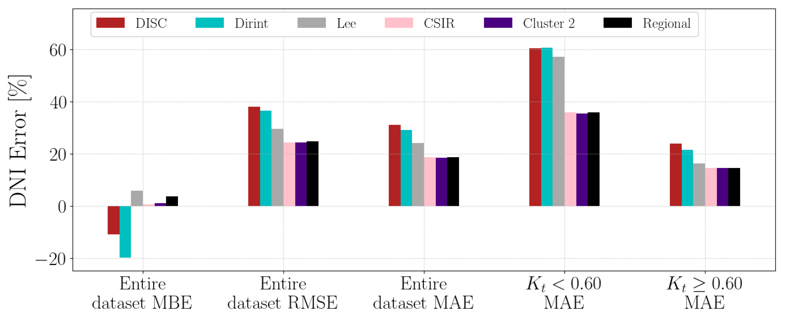
4.1.1. CSIR

Appendix A.1 shows the decomposition model equations for the CSIR station. Table 5 shows the results of the CSIR station. The results show that the localised, Cluster 2 and regional models outperform the baseline models in all metrics. The localised model significantly improves for lower $K_t$, reducing the MAE from around 60% to 36%.

Table 5. Hourly validation results of a decomposition model development for CSIR.

The test results of the CSIR dataset are presented in Figure A1. As seen in the figure, the localised, cluster, and regional models outperform the baseline models, which is consistent with the validation results of the previous section in Table 5.

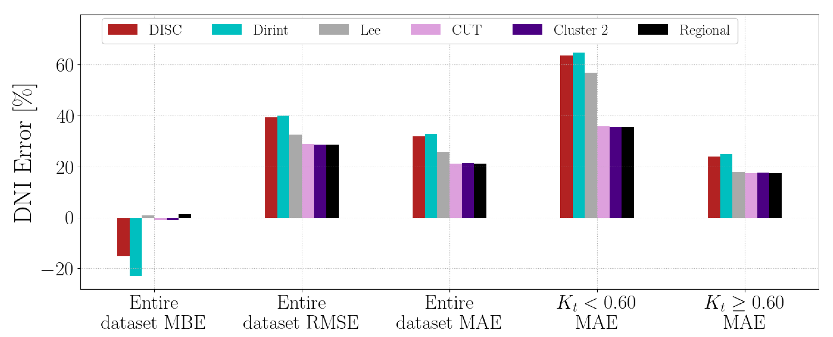
4.1.2. CUT

Appendix A.2 shows the decomposition model equations for the CUT station. Table 6 shows the CUT station results. The localised Cluster 2 and regional model significantly improve the comparison metrics over the three baseline models. The Lee model has a similar MBE to the regional model (±0.7) and has a higher $K_t$-metric similar to Cluster 2. However, the Lee RMSE and MAE still do not outperform the new models.

Table 6. Hourly validation results of decomposition model development for CUT.

Figure A2 presents the test results of the CUT dataset, where the localised, cluster and regional models outperform the baseline models. The test results are consistent with the validation results presented in Table 6.

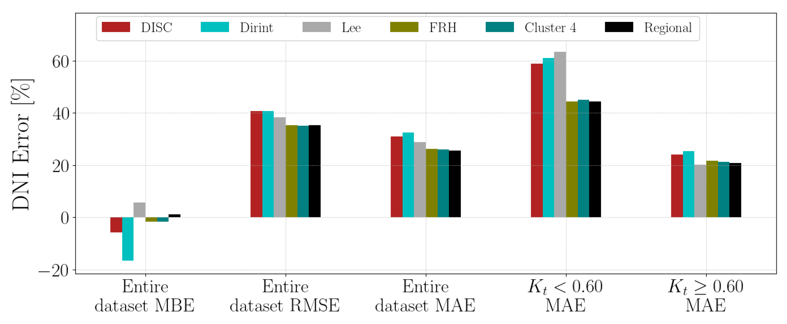
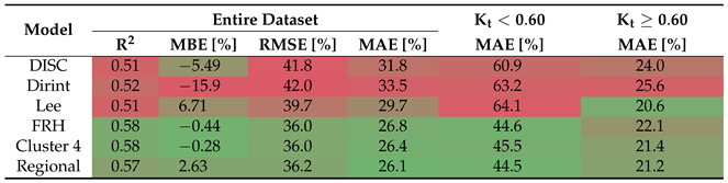
4.1.3. FRH

Appendix A.3 shows the decomposition model equations for the FRH station. Table 7 shows the results of the FRH station. The localised model outperforms the baseline models by improving $R^2$ and MBE and reducing MAE and RSME. The Lee model shows the lowest MAE for higher $K_t$-values; however, it does show an overestimation for DNI with a higher MBE. For most metrics, the localised, Cluster 4 and regional model outperforms the baseline models.

Table 7. Hourly validation results of decomposition model development for FRH.

Figure A3 presents the test results of the FRH dataset. The localised Cluster 2 and regional models outperform the baselines, but no significant difference exists between the three new models. The test results presented in Figure A3 correspond with the validation results in Table 7.

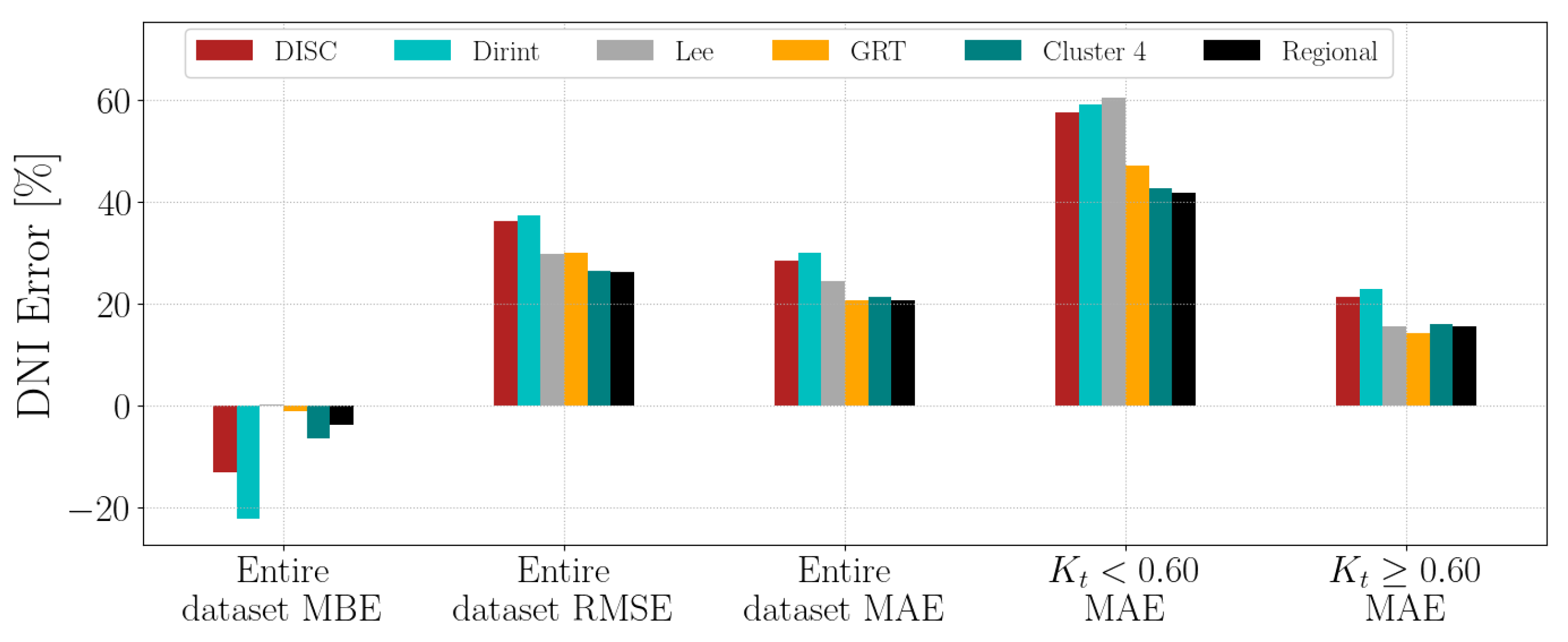
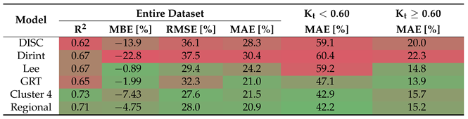
4.1.4. GRT

Appendix A.4 shows the decomposition model equations for the GRT station. Table 8 shows the GRT station results. The localised model does show improvement over the DISC and Dirint model but does not significantly outperform the Lee model. The Lee model has a higher $R^2$ and lower MBE and RMSE, whereas the localised model has a lower MAE for the entire dataset and the two $K_t$ intervals. The Cluster 4 and regional models perform better than the DISC and Dirint models but do not significantly outperform all the baseline models.

Table 8. Hourly validation results of decomposition model development for GRT.

Figure A4 shows the test results of the GRT dataset. The results correspond with the validation results in Table 8. The localised, Cluster 4 and regional model does outperform the DISC and Dirint model but only marginally outperforms the Lee model.

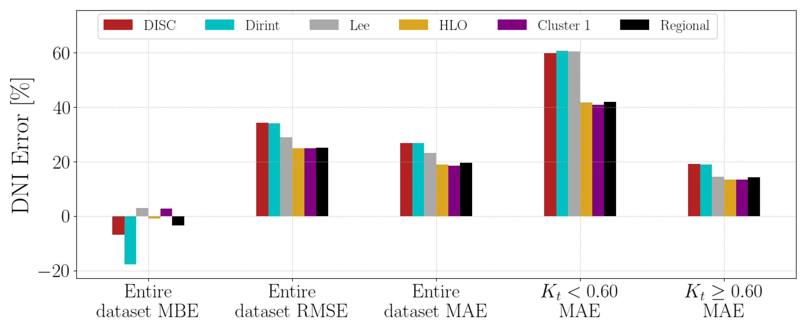
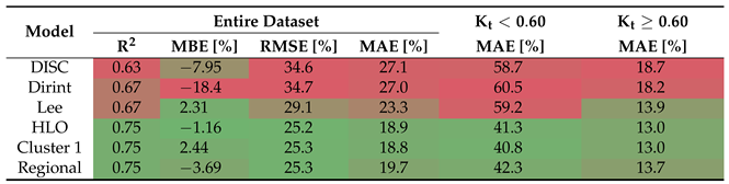
4.1.5. HLO

Appendix A.5 shows the decomposition model equations for the HLO station. Table 9 shows the HLO station results. The localised model performs better than the baseline models and improves all comparison metrics.

Table 9. Hourly validation results of decomposition model development for HLO.

Figure A5 shows the test results of the HLO dataset. The validation results in Table 9 and the test results correspond well, indicating that the localised Cluster 1 and regional models outperform the baseline models.

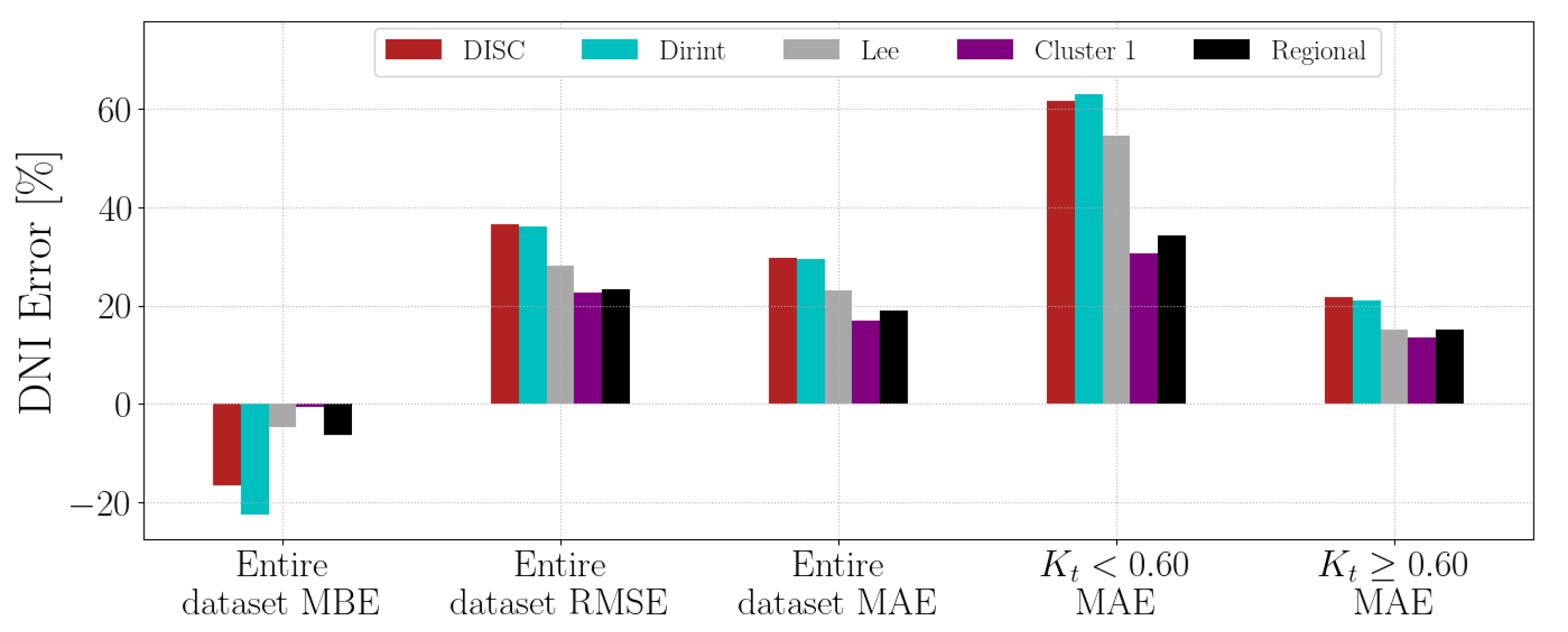
4.1.6. ILA

Figure A6 presents the test results of the ILA dataset. The ILA dataset has no localised decomposition model; therefore, the testing only assesses the Cluster 1 and regional models. The results show that the Cluster 1 and regional models outperform the baseline models. The results highlight the substitution of using a Cluster model when no localised model is available, subject to the geographical location within the Cluster area.

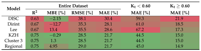
4.1.7. KZH

Appendix A.7 shows the decomposition model equations for the KZH station. Table 10 shows the results of the KZH station. The localised, Cluster 3 and regional models all show significant improvements in reducing the error over the baseline models. The DISC has a lower MBE than the regional model.

Table 10. Hourly validation results of the decomposition model development for KZH.

Figure A7 shows the test results of the KZH dataset. The localised, Cluster 3 and regional models all outperform the baseline models. The regional model does not significantly outperform Cluster 3 or the localised model.

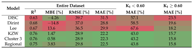
4.1.8. KZW

Appendix A.8 shows the decomposition model equations for the KZW station. Table 11 shows the results of the KZW station. The localised, clustered, and regional models show improvement over the baseline models with metrics that assess the entire dataset.

Table 11. Hourly validation results of decomposition model development for KZW.

Figure A8 shows the test results of the KZW dataset. The validation and testing results from Table 11 correspond.

4.1.9. MIN

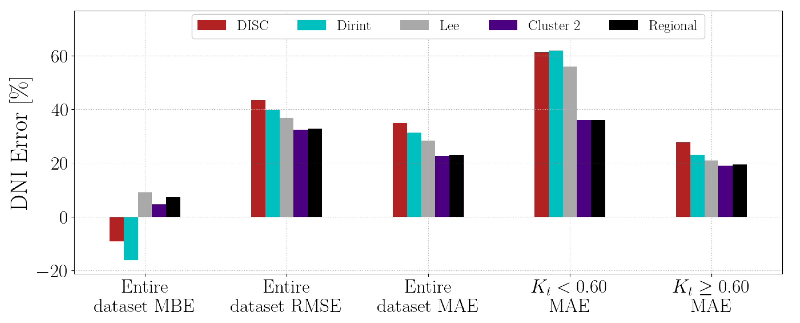
The test results of the MIN dataset are presented in Figure A9. MIN has no localised decomposition model and falls geographically under Cluster 2. The cluster model and localised model show improvement over the baseline models. Much like the ILA dataset, the MIN dataset demonstrates how the clustered and regional models can serve as alternatives to enhance DNI estimations in Southern Africa.

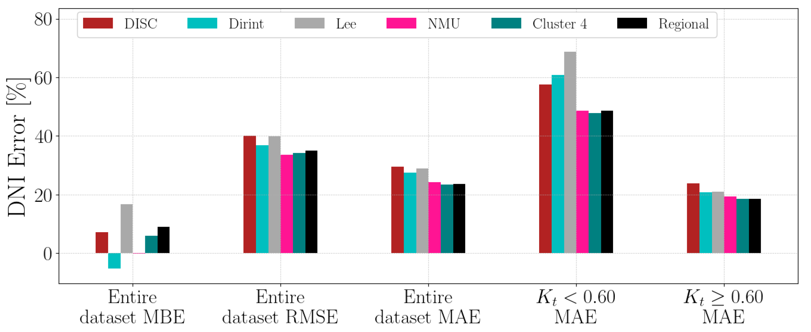
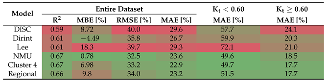
Appendix A.10 shows the decomposition model equations for the NMU station. Table 12 shows the NMU station results. The localised, Cluster 4 and regional models show significant improvement in reducing the errors from the baseline models. Based on the higher MBE, the Cluster 4 and regional models overestimate the DNI more than the DISC and Dirint models.

Table 12. Hourly validation results of decomposition model development for NMU.

The test results of the NMU dataset are presented in Figure A10. Localised and cluster models outperform baseline models, which is consistent with the results in Table 12.

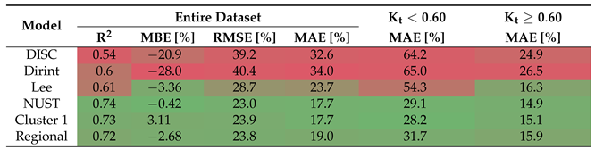
4.1.10. NUST

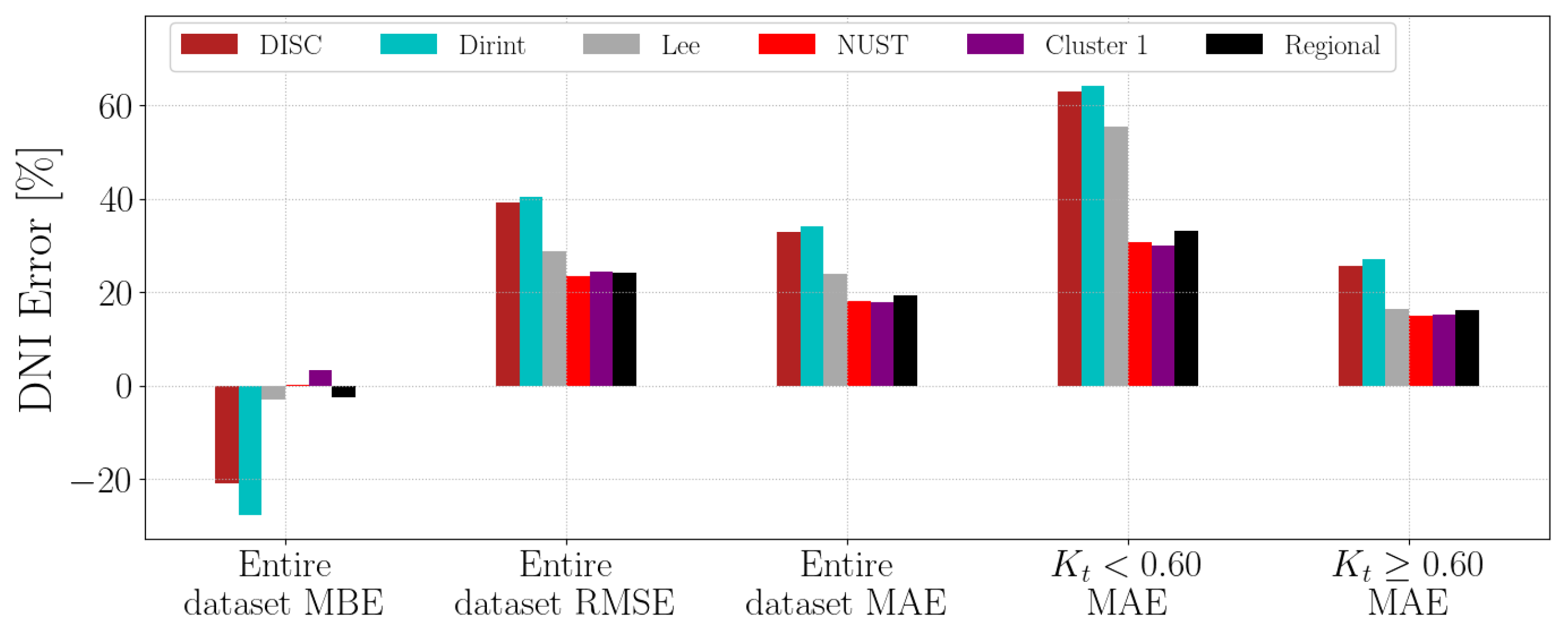
Appendix A.11 shows the decomposition model equations for the NUST station. Table 13 shows the results of the NUST station. The localised model shows superior performance over the baseline models, as well as the clustered and regional models. The metrics of the clustered model compared to the baselines indicate that the regional model slightly overestimates the DNI compared to the lowest baseline model (Lee), which slightly underestimates the DNI.

Table 13. Hourly validation results of decomposition model development for NUST.

The test results of the NUST dataset are presented in Figure A11. Localised, clustered and regional models outperform the baseline models, which is consistent with the validation results presented in Table 13. The regional model shows marginal underperformance compared to the localised and Cluster 1 model, but not significant enough to make it unusable.

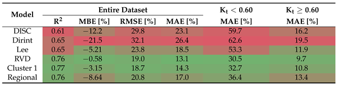
4.1.11. RVD

Appendix A.12 shows the decomposition model equations for the RVD station. Table 14 shows the RVD station results. The localised, clustered and regional models outperform the baseline models. The Lee model performs better than the regional model but does not outperform the localised and cluster models. The RVD station receives more irradiance on average than other stations in the SAURAN database.

Table 14. Hourly validation results of decomposition model development for RVD.

Figure A12 shows the test results of the RVD dataset. The results indicate that the localised, cluster and regional models outperform the baseline models, which is consistent with the validation results of the previous section in Table 14. The localised model’s RMSE is higher than the Lee model; however, the localised model performs best in reducing the error for the other metrics. Though the regional model outperforms the baseline models, it does show the worst performance of the three newly developed models for RVD.

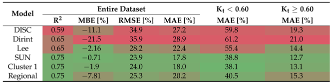
4.1.12. SUN

Appendix A.13 shows the decomposition model equations for the SUN station. Table 15 shows the SUN station results. The localised model outperforms the baseline models by improving $R^2$ and reducing the MBE, RMSE and MAE. The Cluster 1 and regional models show a slightly worse MBE than the Lee baseline model but otherwise outperform the baseline models. The Lee model also predicts higher $K_t$ points with a lower MAE than the regional model; however, the other metrics indicate that the regional model shows better results overall.

Table 15. Hourly validation results of decomposition model development for SUN.

Figure A13 shows the test results of the SUN dataset. The results indicate that the localised, cluster and regional models outperform the baseline models, which is consistent with the testing results of the previous section in Table 15. As with the validation results, the regional model is the worst-performing new model, but it still outperforms the baseline models.

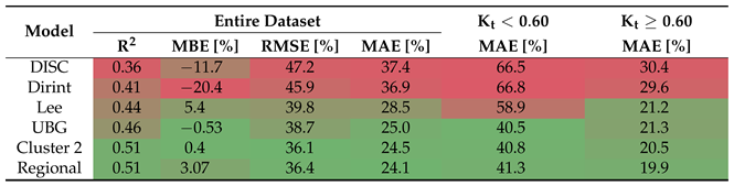
4.1.13. UBG

Appendix A.14 shows the decomposition model equations for the UBG station. Table 16 shows the UBG station results. The localised, clustered and regional models all outperform the baseline models. The Lee model has a lower MBE than the Cluster 1 and regional models. The Lee model also has a lower MAE for $K_t\ge 0.60$; however, the other metrics indicate that the model does not improve the $R^2$, RMSE, overall MAE or $K_t<0.60$ MAE.

Table 16. Hourly validation results of decomposition model development for UBG.

Figure A14 shows the test results of the UBG dataset. The test results show that the localised, Cluster 1 and regional models outperform the baseline models. The Lee model has a lower MBE than the regional model, which is consistent with the validation results in Table 16.

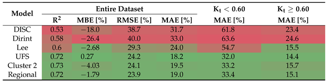
4.1.14. UFS

Appendix A.15 shows the decomposition model equations for the UFS station. Table 17 shows the UFS station results. The localised, Cluster 2 and regional models outperform the baseline models. The Lee model underestimates the DNI slightly better than the Cluster 2 model.

Table 17. Hourly validation results of decomposition model development for UFS.

Figure A15 shows the test results of the UFS dataset. All three new decomposition models significantly improve the errors compared to the baseline models, which is consistent with the validation results in Table 17.

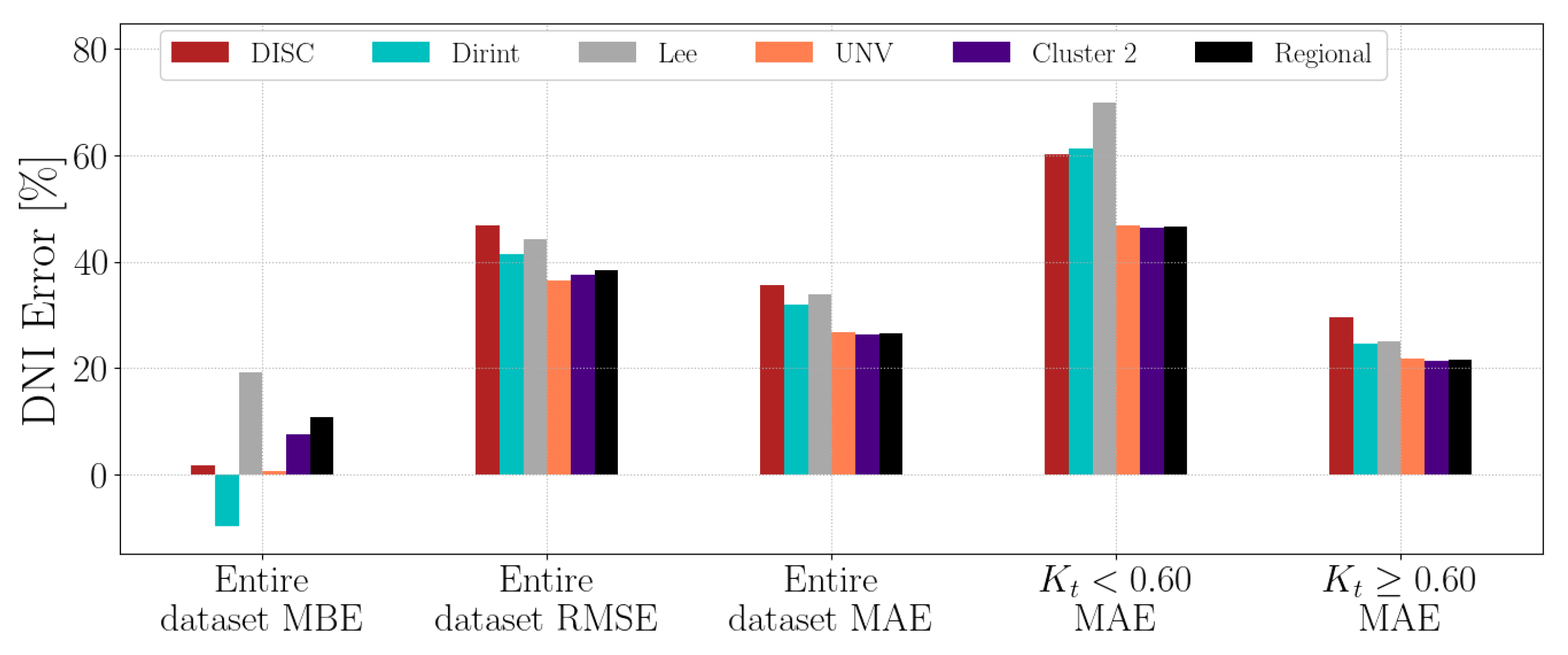
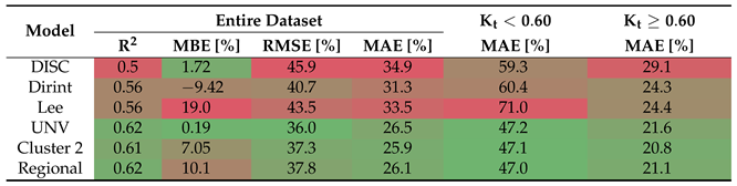
4.1.15. UNV

Appendix A.16 shows the decomposition model equations for the UNV station. Table 18 shows the UNV station results. The localised, Cluster 2 and regional models significantly improved over the baseline models. The Cluster 2 and regional model overestimates the DNI more than the DISC model, based on the MBE.

Table 18. Hourly validation results of decomposition model development for UNV.

Figure A16 shows the test results of the UNV dataset. The test results correspond with the validation results in Table 18, where the localised, Cluster 2 and regional models outperform the baseline models. The only exception is the MBE, where the Cluster 2 and regional models perform worse than the DISC model. Considering all the metrics, the new models outperform the baselines in reducing the overall error of DNI estimations.

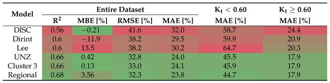
4.1.16. UNZ

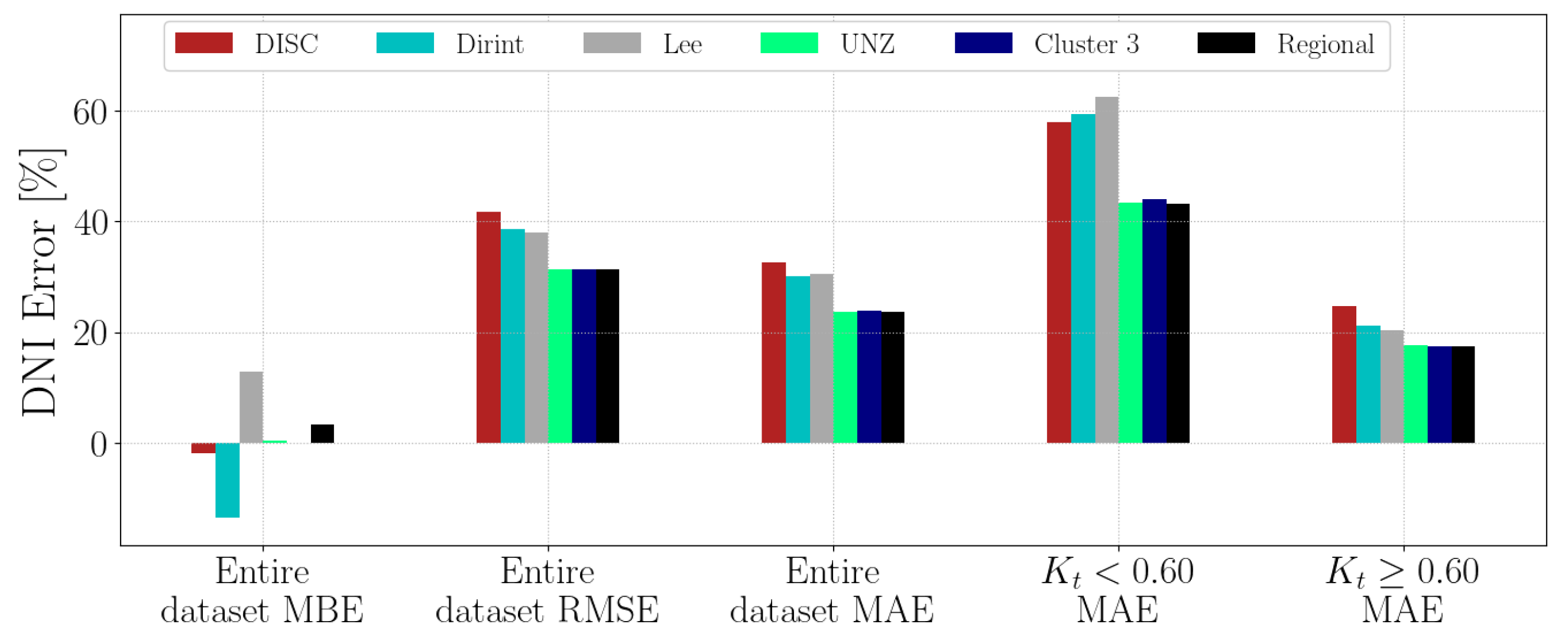
Appendix A.17 shows the decomposition model equations for the UNZ station. Table 19 shows the results of the UNZ station. The localised, clustered and regional models all show improvement over the baselines. The Dirint model has a lower MBE than the regional model.

Table 19. Hourly validation results of the decomposition model development for UNZ.

Figure A17 shows the test results of the UNZ dataset, which correspond with the validation results in Table 19.

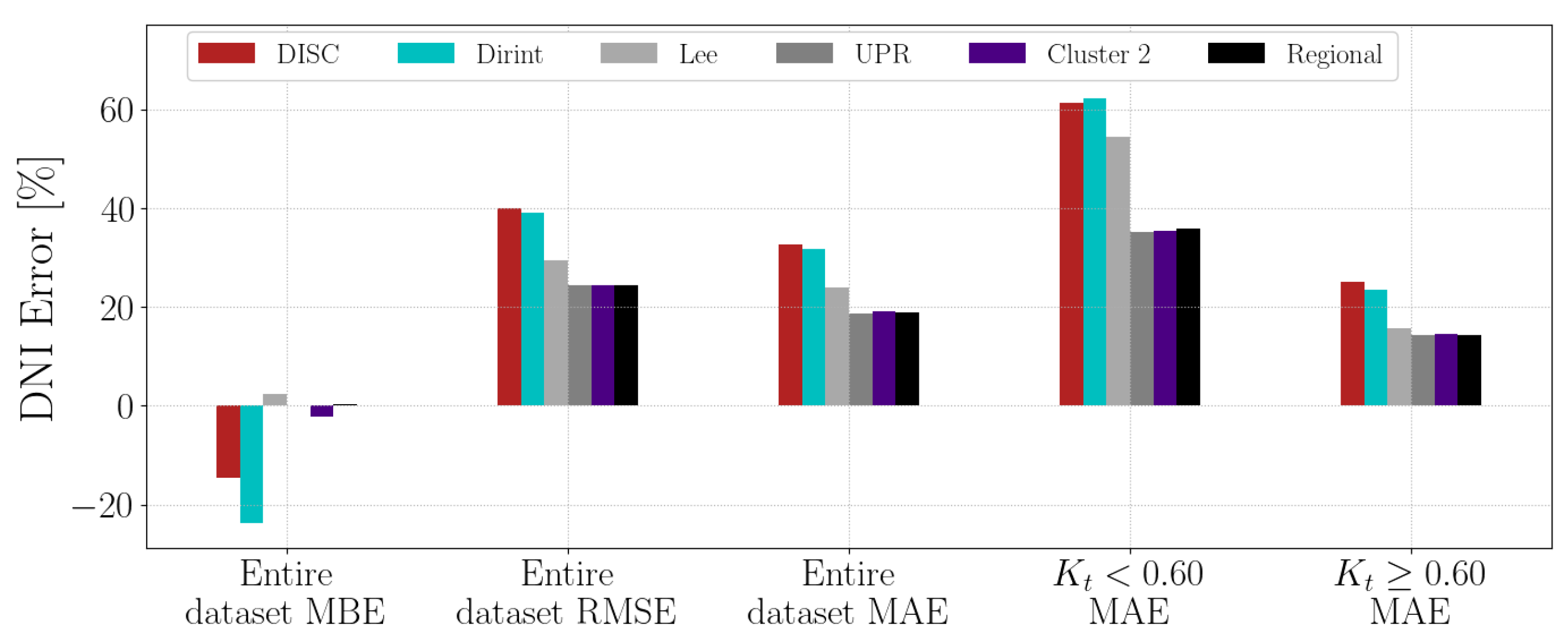
4.1.17. UPR

Appendix A.18 shows the decomposition model equations for the UPR station. Table 20 shows the UPR station results. The localised, cluster and regional models outperform the baseline models.

Table 20. Hourly validation results of decomposition model development for UPR.

Figure A18 shows the test results of the UPR dataset. The comparison metrics of the entire dataset indicate that the localised, cluster and regional models outperform the baseline models, which is consistent with the results of the validation dataset in Table 20.

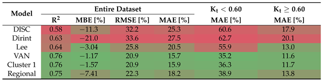
4.1.18. VAN

Appendix A.19 shows the decomposition model equations for the VAN station. Table 21 shows the results of the VAN station. The localised model outperforms the baseline models by improving $R^2$ and reducing the MBE, RMSE and MAE. The new models significantly reduce the MAE in the higher $K_t$ compared to the baseline models. Even when outperforming the baseline models, the regional model performs worse than the new model. The VAN station receives a very high average DNI and DHI and lower DHI than the rest of the database’s stations. These results are similar to the RVD station, which has significantly higher irradiance levels than the other stations.

Table 21. Hourly validation results of decomposition model development for VAN.

Figure A19 shows the test results of the VAN dataset. The new models all outperform the baseline models. The regional model shows the worst performance of the new models, even when outperforming the baseline models, similar to the RVD station that receives more irradiance on average compared to the other stations. These results are consistent with the validation results in Table 21.

4.2. Discussion

Table 22 summarises the performance of the localised, clustered and regional models for both the test and validation sets.

Table 22. Summary of test and validation sets of stations outperforming baseline models.

Dataset	Localised Model Outperforms Baseline Models		Cluster Model Outperforms Baseline ModelsBaseline Models		Regional Model Outperforms Baseline Models
	Test	Validation	Test	Validation	Test	Validation
CSIR	✓	✓	✓	✓	✓	✓
CUT	✓	✓	✓	✓	✓	✓
FRH	✓	✓	✓	✓	✓	✓
GRT	✓	✓	✓	✓	✓	✓
HLO	✓	✓	✓	✓	✓	✓
ILA	-	✓	-	✓	-	✓
KZH	✓	✓	✓	✓	✓	✓
KZW	✓	✓	✓	✓	✓	✓
MIN	-	✓	-	✓	-	✓
NMU	✓	✓	✓	✓	✓	✓
NUST	✓	✓	✓	✓	✓	✓
RVD	✓	✓	✓	✓	✓	✓
SUN	✓	✓	✓	✓	✓	✓
UBG	✓	✓	✓	✓	✓	✓
UFS	✓	✓	✓	✓	✓	✓
UNV	✓	✓	✓	✓	✓	✓
UNZ	✓	✓	✓	✓	✓	✓
UPR	✓	✓	✓	✓	✓	✓
VAN	✓	✓	✓	✓	✓	✓

As expected, the localised models outperformed the baseline models for all station datasets because of the site-specific climatic training data. As discussed in the previous section, the cluster model combines multiple stations in a similar geographical area.

The clustered model will have significantly more data from which to train a model. A clustered model is ideal if a site has no data for localised model development using the discussed methodology. The regional (Southern African) model also shows improvement over the baseline models, indicating that this model may be appropriate for adoption as a new model for Southern Africa. The two models with no localised models (ILA and MIN) showed improvement using the clustered and regional models in the validation study.

5. Conclusions

This article presents the development of a new decomposition model of hourly DNI estimations for Southern Africa using the SAURAN database. The new models improved the DISC model in developing new decomposition models localised for Southern African climates. The new decomposition models significantly improved the DNI estimation errors over the baselines for all the SAURAN stations’ validation and test data sets. The proposed methodology can be helpful for the development of local decomposition models for other areas worldwide.

The results indicate that a localised model will improve the estimations of DNI. Clustered models also indicate that grouping data based on similar geographical and climatic properties can also improve the performance of decomposition models. This phenomenon could be helpful when using a clustered decomposition model if no local model or limited data are available but are available from two or more geographically close stations.

The overall model, the regional decomposition model, is encapsulated by different climatic regions and geographical locations. There are also some exceptions where the model over- or underestimates the DNI; however, the overall metrics indicate that the Southern African model significantly improves over the baseline models.

The validation study conducted at two stations further substantiates the superiority of the developed hourly decomposition models over comparative models, emphasising their robustness and applicability in realistic scenarios where the localised models are usually not unavailable. The study validates hourly irradiance data for $K_t$ intervals between 0.175 and 0.875. Recommendations for future work include developing models for higher and lower $K_t$ values and models for higher temporal resolutions with increased accuracy, which is ideal for the real-time monitoring and short-term forecasting of PV power.

Developing countries with an accurate decomposition model can open the path to expanding the use of renewable energy sources and reducing their dependence on coal and fossil fuels. Good-quality data are needed to ensure the progress of research and development related ot solar energy, and this paper addresses the shortcomings of the Southern African region’s lack of accurate solar resource representation in existing models. The next step is assessing the decomposition models with well-known transposition models to determine improved accuracy for PR estimations.

Appendix A.1. CSIR

The a, b and c coefficients for Equation (34) for the CSIR station are

$$\begin{array}{cc}\hfill a& =\left\{\begin{array}{c}0.6472-1.0883K_t+12.3429K_t^2-17.7027K_t^3\mathrm{for}{K}_t<0.60,\hfill \\ 6.1444-9.484K_t-5.138K_t^2+9.2371K_t^3\mathrm{for}{K}_t\ge 0.60.\hfill \end{array}\right.\hfill \\ \hfill b& =\left\{\begin{array}{c}-0.5032+5.67K_t-22.0707K_t^2+22.2654K_t^3\mathrm{for}{K}_t<0.60,\hfill \\ 2.8669-22.2584K_t+43.4833K_t^2-24.9682K_t^3\mathrm{for}{K}_t\ge 0.60.\hfill \end{array}\right.\hfill \\ \hfill c& =\left\{\begin{array}{c}0.1418-1.4904K_t+4.7805K_t^2-4.3489K_t^3\mathrm{for}{K}_t<0.60,\hfill \\ -1.1287+5.8459K_t-9.4568K_t^2+4.8729K_t^3\mathrm{for}{K}_t\ge 0.60.\hfill \end{array}\right.\hfill \end{array}$$

(A1)

The test results of the CSIR dataset are in Figure A1.

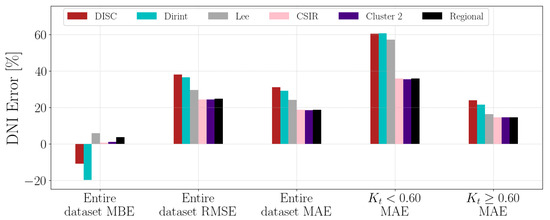
Figure A1. Hourly test results of decomposition model development for CSIR.

Figure A1. Hourly test results of decomposition model development for CSIR.

Appendix A.2. CUT

The a, b and c coefficients for Equation (34) for the CUT station are

$$\begin{array}{cc}\hfill a& =\left\{\begin{array}{c}2.4122-15.382K_t+48.3773K_t^2-45.8766K_t^3\mathrm{for}{K}_t<0.60,\hfill \\ -15.7689+86.1878K_t-141.6902K_t^2+73.2142K_t^3\mathrm{for}{K}_t\ge 0.60.\hfill \end{array}\right.\hfill \\ \hfill b& =\left\{\begin{array}{c}-1.6214+14.8897K_t-45.5364K_t^2+40.6731K_t^3\mathrm{for}{K}_t<0.60,\hfill \\ 17.2881-85.5492K_t+134.0146K_t^2-67.4052K_t^3\mathrm{for}{K}_t\ge 0.60.\hfill \end{array}\right.\hfill \\ \hfill c& =\left\{\begin{array}{c}0.2864-2.6906K_t+7.8329K_t^2-6.7318K_t^3\mathrm{for}{K}_t<0.60,\hfill \\ -1.9147+9.6635K_t-15.3053K_t^2+7.7563K_t^3\mathrm{for}{K}_t\ge 0.60.\hfill \end{array}\right.\hfill \end{array}$$

(A2)

The validation results of the CUT dataset are in Figure A2.

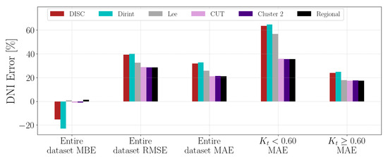
Figure A2. Hourly test results of decomposition model development for CUT.

Figure A2. Hourly test results of decomposition model development for CUT.

Appendix A.3. FRH

The a, b and c coefficients for Equation (34) for the FRH station are

$$\begin{array}{cc}\hfill a& =\left\{\begin{array}{c}1.3199-6.0578K_t+24.6953K_t^2-27.3825K_t^3\mathrm{for}{K}_t<0.60,\hfill \\ 33.3782-124.5221K_t+155.5513K_t^2-64.7203K_t^3\mathrm{for}{K}_t\ge 0.60.\hfill \end{array}\right.\hfill \\ \hfill b& =\left\{\begin{array}{c}-0.5658+5.6247K_t-21.3334K_t^2+21.2952K_t^3\mathrm{for}{K}_t<0.60,\hfill \\ -26.2959+102.0318K_t-131.6271K_t^2+56.3592K_t^3\mathrm{for}{K}_t\ge 0.60.\hfill \end{array}\right.\hfill \\ \hfill c& =\left\{\begin{array}{c}0.0963-1.024K_t+3.5042K_t^2-3.2887K_t^3\mathrm{for}{K}_t<0.60,\hfill \\ 3.9117-15.5175K_t+20.4822K_t^2-8.9754K_t^3\mathrm{for}{K}_t\ge 0.60.\hfill \end{array}\right.\hfill \end{array}$$

(A3)

The test results of the FRH dataset are in Figure A3.

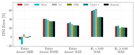
Figure A3. Hourly test results of decomposition model development for FRH.

Figure A3. Hourly test results of decomposition model development for FRH.

Appendix A.4. GRT

The a, b and c coefficients for Equation (34) for the GRT station are

$$\begin{array}{c}\hfill a=\left\{\begin{array}{c}2.9602-19.6392K_t+58.9738K_t^2-55.4505K_t^3\mathrm{for}{K}_t<0.60,\hfill \\ -29.0697+138.0498K_t-209.2486K_t^2+102.455K_t^3\mathrm{for}{K}_t\ge 0.60.\hfill \end{array}\right.\\ \hfill b=\left\{\begin{array}{c}-2.2843+20.1509K_t-58.384K_t^2+51.362K_t^3\mathrm{for}{K}_t<0.60,\hfill \\ 34.8693-155.9554K_t+227.6821K_t^2-108.7518K_t^3\mathrm{for}{K}_t\ge 0.60.\hfill \end{array}\right.\\ \hfill c=\left\{\begin{array}{c}0.4656-4.1668K_t+11.5129K_t^2-9.7101K_t^3\mathrm{for}{K}_t<0.60,\hfill \\ -8.4664+36.6029K_t-51.9382K_t^2+24.2327K_t^3\mathrm{for}{K}_t\ge 0.60.\hfill \end{array}\right.\end{array}$$

(A4)

Figure A4 shows the test results of the GRT dataset.

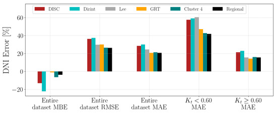
Figure A4. Hourly test results of decomposition model development for GRT.

Figure A4. Hourly test results of decomposition model development for GRT.

Appendix A.5. HLO

The a, b and c coefficients for Equation (34) for the HLO station are

$$\begin{array}{c}\hfill a=\left\{\begin{array}{c}3.1156-21.0151K_t+62.5312K_t^2-57.2369K_t^3\mathrm{for}{K}_t<0.60,\hfill \\ 50.8058-194.5525K_t+248.2624K_t^2-105.3977K_t^3\mathrm{for}{K}_t\ge 0.60.\hfill \end{array}\right.\\ \hfill b=\left\{\begin{array}{c}-2.0533+18.2104K_t-53.4859K_t^2+46.7754K_t^3\mathrm{for}{K}_t<0.60,\hfill \\ -33.1822+128.4612K_t-164.8983K_t^2+70.2185K_t^3\mathrm{for}{K}_t\ge 0.60.\hfill \end{array}\right.\\ \hfill c=\left\{\begin{array}{c}0.3508-3.2108K_t+9.1319K_t^2-7.7849K_t^3\mathrm{for}{K}_t<0.60,\hfill \\ 3.7247-14.4408K_t+18.5853K_t^2-7.9382K_t^3\mathrm{for}{K}_t\ge 0.60.\hfill \end{array}\right.\end{array}$$

(A5)

Figure A5 shows the test results of the HLO dataset.

Figure A5. Hourly test results of decomposition model development for HLO.

Figure A5. Hourly test results of decomposition model development for HLO.

Appendix A.6. ILA

There is no decomposition model developed for the ILA station.

The test results of the ILA dataset are in Figure A6.

Figure A6. Hourly test results of decomposition model development for ILA.

Figure A6. Hourly test results of decomposition model development for ILA.

Appendix A.7. KZH

The a, b and c coefficients for Equation (34) for the KZH station are

$$\begin{array}{c}\hfill a=\left\{\begin{array}{c}1.3444-6.1333K_t+23.7139K_t^2-25.5604K_t^3\mathrm{for}{K}_t<0.60,\hfill \\ 56.4073-216.3047K_t+276.4264K_t^2-117.5281K_t^3\mathrm{for}{K}_t\ge 0.60.\hfill \end{array}\right.\\ \hfill b=\left\{\begin{array}{c}-0.7156+6.8854K_t-24.0569K_t^2+22.9604K_t^3\mathrm{for}{K}_t<0.60,\hfill \\ -45.6353+178.5713K_t-231.593K_t^2+99.6179K_t^3\mathrm{for}{K}_t\ge 0.60.\hfill \end{array}\right.\\ \hfill c=\left\{\begin{array}{c}0.1646-1.6569K_t+5.2451K_t^2-4.7368K_t^3\mathrm{for}{K}_t<0.60,\hfill \\ 6.2156-24.5162K_t+32.0741K_t^2-13.9205K_t^3\mathrm{for}{K}_t\ge 0.60.\hfill \end{array}\right.\end{array}$$

(A6)

The test results of the KZH dataset are in Figure A7.

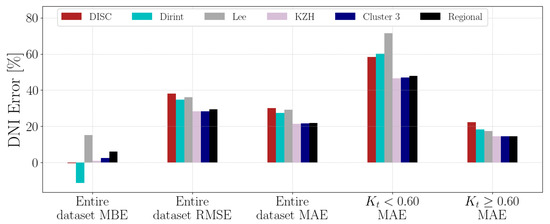
Figure A7. Hourly test results of decomposition model development for KZH.

Figure A7. Hourly test results of decomposition model development for KZH.

Appendix A.8. KZW

The a, b and c coefficients for Equation (34) for the KZW station are

$$\begin{array}{c}\hfill a=\left\{\begin{array}{c}2.2627-14.4806K_t+47.1629K_t^2-46.2386K_t^3\mathrm{for}{K}_t<0.60,\hfill \\ 35.0603-132.558K_t+167.2728K_t^2-70.2359K_t^3\mathrm{for}{K}_t\ge 0.60.\hfill \end{array}\right.\\ \hfill b=\left\{\begin{array}{c}-1.4332+13.4317K_t-42.4822K_t^2+39.1838K_t^3\mathrm{for}{K}_t<0.60,\hfill \\ -28.1708+109.9004K_t-141.9142K_t^2+60.6943K_t^3\mathrm{for}{K}_t\ge 0.60.\hfill \end{array}\right.\\ \hfill c=\left\{\begin{array}{c}0.2678-2.6116K_t+7.9363K_t^2-7.1072K_t^3\mathrm{for}{K}_t<0.60,\hfill \\ 3.1759-12.4602K_t+16.1949K_t^2-6.9726K_t^3\mathrm{for}{K}_t\ge 0.60.\hfill \end{array}\right.\end{array}$$

(A7)

Figure A8 shows the test results of the KZW dataset.

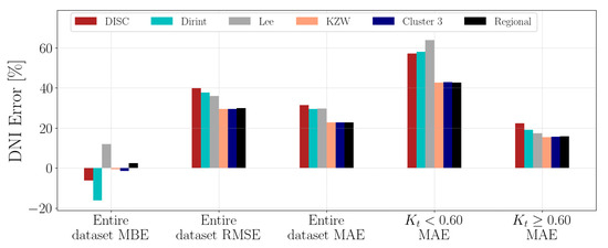
Figure A8. Hourly test results of decomposition model development for KZW.

Figure A8. Hourly test results of decomposition model development for KZW.

Appendix A.9. MIN

There is no decomposition model developed for the MIN station.

The test results of the MIN dataset are in Figure A9.

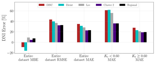
Figure A9. Hourly test results of decomposition model development for MIN.

Figure A9. Hourly test results of decomposition model development for MIN.

Appendix A.10. NMU

The a, b and c coefficients for Equation (34) for the NMU station are

$$\begin{array}{c}\hfill a=\left\{\begin{array}{c}0.0688+5.2168K_t-7.122K_t^2+0.2163K_t^3\mathrm{for}{K}_t<0.60,\hfill \\ 15.7683-48.8606K_t+48.5956K_t^2-15.0438K_t^3\mathrm{for}{K}_t\ge 0.60.\hfill \end{array}\right.\\ \hfill b=\left\{\begin{array}{c}0.3483-2.9436K_t+3.2778K_t^2-0.0145K_t^3\mathrm{for}{K}_t<0.60,\hfill \\ -11.0783+37.046K_t-39.8763K_t^2+13.6687K_t^3\mathrm{for}{K}_t\ge 0.60.\hfill \end{array}\right.\\ \hfill c=\left\{\begin{array}{c}-0.0758+0.598K_t-1.1265K_t^2+0.7025K_t^3\mathrm{for}{K}_t<0.60,\hfill \\ 1.9782-7.2272K_t+8.7285K_t^2-3.4834K_t^3\mathrm{for}{K}_t\ge 0.60.\hfill \end{array}\right.\end{array}$$

(A8)

The test results of the NMU dataset are in Figure A10.

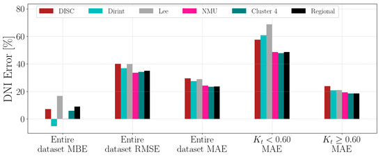
Figure A10. Hourly test results of decomposition model development for NMU.

Figure A10. Hourly test results of decomposition model development for NMU.

Appendix A.11. NUST

The a, b and c coefficients for Equation (34) for the NUST station are

$$\begin{array}{cc}\hfill a& =\left\{\begin{array}{c}2.0021-11.1478K_t+36.3216K_t^2-35.8544K_t^3\mathrm{for}{K}_t<0.60,\hfill \\ -17.9917+91.7087K_t-144.5222K_t^2+72.3519K_t^3\mathrm{for}{K}_t\ge 0.60.\hfill \end{array}\right.\hfill \\ \hfill b& =\left\{\begin{array}{c}-1.2658+11.3567K_t-35.6964K_t^2+32.4545K_t^3\mathrm{for}{K}_t<0.60,\hfill \\ 24.1237-111.1616K_t+165.4905K_t^2-79.997K_t^3\mathrm{for}{K}_t\ge 0.60,\hfill \end{array}\right.\hfill \\ \hfill c& =\left\{\begin{array}{c}0.2056-1.9277K_t+5.7745K_t^2-5.0518K_t^3\mathrm{for}{K}_t<0.60,\hfill \\ -2.59+11.8847K_t-17.6199K_t^2+8.4894K_t^3\mathrm{for}{K}_t\ge 0.60.\hfill \end{array}\right.\hfill \end{array}$$

(A9)

The test results of the NUST dataset are in Figure A11.

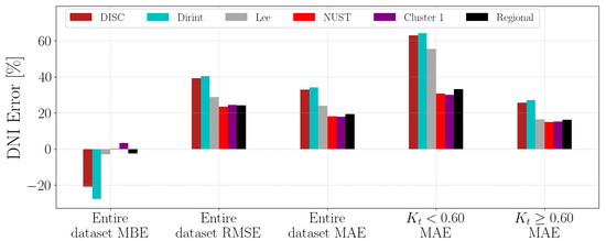
Figure A11. Hourly test results of decomposition model development for NUST.

Figure A11. Hourly test results of decomposition model development for NUST.

Appendix A.12. RVD

The a, b and c coefficients for Equation (34) for the RVD station are

$$\begin{array}{cc}\hfill a& =\left\{\begin{array}{c}4.0191-28.309K_t+83.0024K_t^2-74.0684K_t^3\mathrm{for}{K}_t<0.60,\hfill \\ 84.2546-327.2114K_t+422.3587K_t^2-181.2345K_t^3\mathrm{for}{K}_t\ge 0.60.\hfill \end{array}\right.\hfill \\ \hfill b& =\left\{\begin{array}{c}-2.8895+25.4823K_t-74.043K_t^2+63.2378K_t^3\mathrm{for}{K}_t<0.60,\hfill \\ -65.5943+256.2577K_t-331.9301K_t^2+142.7166K_t^3\mathrm{for}{K}_t\ge 0.60.\hfill \end{array}\right.\hfill \\ \hfill c& =\left\{\begin{array}{c}0.5456-4.9199K_t+13.8139K_t^2-11.415K_t^3\mathrm{for}{K}_t<0.60,\hfill \\ 10.4557-41.161K_t+53.7847K_t^2-23.3378K_t^3\mathrm{for}{K}_t\ge 0.60.\hfill \end{array}\right.\hfill \end{array}$$

(A10)

The test results of the RVD dataset are in Figure A12.

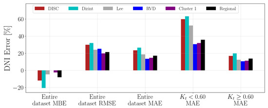
Figure A12. Hourly test results of decomposition model development for RVD.

Figure A12. Hourly test results of decomposition model development for RVD.

Appendix A.13. SUN

The a, b and c coefficients for Equation (34) for the SUN station are

$$\begin{array}{c}\hfill a=\left\{\begin{array}{c}1.4996-7.646K_t+30.0235K_t^2-33.6216K_t^3\mathrm{for}{K}_t<0.60,\hfill \\ 32.6225-122.3879K_t+152.4023K_t^2-62.9667K_t^3\mathrm{for}{K}_t\ge 0.60.\hfill \end{array}\right.\\ \hfill b=\left\{\begin{array}{c}-0.835+7.9823K_t-28.5353K_t^2+28.4965K_t^3\mathrm{for}{K}_t<0.60,\hfill \\ -19.4403+73.2046K_t-90.6277K_t^2+36.9662K_t^3\mathrm{for}{K}_t\ge 0.60.\hfill \end{array}\right.\\ \hfill c=\left\{\begin{array}{c}0.1285-1.3014K_t+4.3214K_t^2-4.0834K_t^3\mathrm{for}{K}_t<0.60,\hfill \\ 2.0866-7.7979K_t+9.595K_t^2-3.8902K_t^3\mathrm{for}{K}_t\ge 0.60.\hfill \end{array}\right.\end{array}$$

(A11)

The test results of the SUN dataset are in Figure A13.

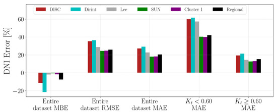
Figure A13. Hourly test results of decomposition model development for SUN.

Figure A13. Hourly test results of decomposition model development for SUN.

Appendix A.14. UBG

The a, b and c coefficients for Equation (34) for the UBG station are

$$\begin{array}{c}\hfill a=\left\{\begin{array}{c}0.5601+1.4348K_t+1.9992K_t^2-6.4178K_t^3\mathrm{for}{K}_t<0.60,\hfill \\ 42.1623-152.8269K_t+183.6564K_t^2-73.01K_t^3\mathrm{for}{K}_t\ge 0.60.\hfill \end{array}\right.\\ \hfill b=\left\{\begin{array}{c}-0.0378+0.6077K_t-6.2716K_t^2+7.0084K_t^3\mathrm{for}{K}_t<0.60,\hfill \\ -44.4913+167.9403K_t-209.5344K_t^2+86.5114K_t^3\mathrm{for}{K}_t\ge 0.60.\hfill \end{array}\right.\\ \hfill c=\left\{\begin{array}{c}0.0159-0.2605K_t+1.1245K_t^2-0.8877K_t^3\mathrm{for}{K}_t<0.60,\hfill \\ 9.2841-35.956K_t+46.1639K_t^2-19.6586K_t^3\mathrm{for}{K}_t\ge 0.60.\hfill \end{array}\right.\end{array}$$

(A12)

The test results of the SUN dataset are in Figure A14.

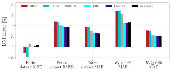
Figure A14. Hourly test results of decomposition model development for UBG.

Figure A14. Hourly test results of decomposition model development for UBG.

Appendix A.15. UFS

The a, b and c coefficients for Equation (34) for the UFS station are

$$\begin{array}{c}\hfill a=\left\{\begin{array}{c}1.1152-5.4355K_t+27.3687K_t^2-32.6276K_t^3\mathrm{for}{K}_t<0.60,\hfill \\ 18.8962-58.0528K_t+56.4791K_t^2-16.8735K_t^3\mathrm{for}{K}_t\ge 0.60.\hfill \end{array}\right.\\ \hfill b=\left\{\begin{array}{c}-0.5439+6.5875K_t-27.7113K_t^2+28.8812K_t^3\mathrm{for}{K}_t<0.60,\hfill \\ -19.1711+65.1123K_t-71.8324K_t^2+25.6916K_t^3\mathrm{for}{K}_t\ge 0.60.\hfill \end{array}\right.\\ \hfill c=\left\{\begin{array}{c}0.1395-1.6147K_t+5.7356K_t^2-5.4904K_t^3\mathrm{for}{K}_t<0.60,\hfill \\ 5.238-19.7369K_t+24.6715K_t^2-10.2415K_t^3\mathrm{for}{K}_t\ge 0.60.\hfill \end{array}\right.\end{array}$$

(A13)

The test results of the SUN dataset are in Figure A15.

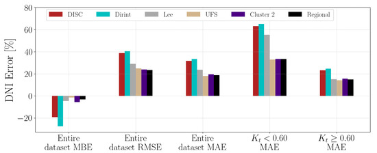
Figure A15. Hourly test results of decomposition model development for UFS.

Figure A15. Hourly test results of decomposition model development for UFS.

Appendix A.16. UNV

The a, b and c coefficients for Equation (34) for the UNV station are

$$\begin{array}{c}\hfill a=\left\{\begin{array}{c}1.6679-8.8496K_t+30.8258K_t^2-31.7801K_t^3\mathrm{for}{K}_t<0.60,\hfill \\ 17.0947-58.7362K_t+67.3532K_t^2-25.6036K_t^3\mathrm{for}{K}_t\ge 0.60.\hfill \end{array}\right.\\ \hfill b=\left\{\begin{array}{c}-0.9329+8.8795K_t-29.6546K_t^2+28.1554K_t^3\mathrm{for}{K}_t<0.60,\hfill \\ -11.0559+39.0859K_t-45.1859K_t^2+17.0921K_t^3\mathrm{for}{K}_t\ge 0.60.\hfill \end{array}\right.\\ \hfill c=\left\{\begin{array}{c}0.1744-1.744K_t+5.4271K_t^2-4.9023K_t^3\mathrm{for}{K}_t<0.60,\hfill \\ 0.7738-2.5106K_t+2.5888K_t^2-0.8303K_t^3\mathrm{for}{K}_t\ge 0.60.\hfill \end{array}\right.\end{array}$$

(A14)

The test results of the UNV dataset are in Figure A16.

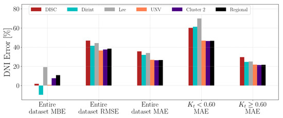
Figure A16. Hourly test results of decomposition model development for UNV.

Figure A16. Hourly test results of decomposition model development for UNV.

Appendix A.17. UNZ

The a, b and c coefficients for Equation (34) for the UNZ station are

$$\begin{array}{c}\hfill a=\left\{\begin{array}{c}1.1129-5.2859K_t+25.5284K_t^2-30.5998K_t^3\mathrm{for}{K}_t<0.60,\hfill \\ 33.4179-127.1391K_t+161.8637K_t^2-68.7679K_t^3\mathrm{for}{K}_t\ge 0.60.\hfill \end{array}\right.\\ \hfill b=\left\{\begin{array}{c}-0.6222+7.0597K_t-28.1112K_t^2+29.4187K_t^3\mathrm{for}{K}_t<0.60,\hfill \\ -24.1838+94.1721K_t-121.4204K_t^2+51.9098K_t^3\mathrm{for}{K}_t\ge 0.60.\hfill \end{array}\right.\\ \hfill c=\left\{\begin{array}{c}0.1398-1.5931K_t+5.5902K_t^2-5.4749K_t^3\mathrm{for}{K}_t<0.60,\hfill \\ 2.3838-9.2877K_t+11.9991K_t^2-5.1432K_t^3\mathrm{for}{K}_t\ge 0.60.\hfill \end{array}\right.\end{array}$$

(A15)

The test results of the UNZ dataset are in Figure A17.

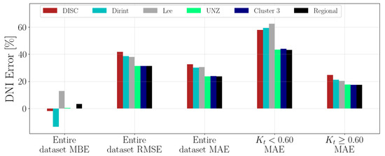
Figure A17. Hourly test results of decomposition model development for UNZ.

Figure A17. Hourly test results of decomposition model development for UNZ.

Appendix A.18. UPR

The a, b and c coefficients for Equation (34) for the UPR station are

$$\begin{array}{c}\hfill a=\left\{\begin{array}{c}1.3766-6.4439K_t+25.7243K_t^2-28.9372K_t^3\mathrm{for}{K}_t<0.60,\hfill \\ -2.5908+24.5466K_t-49.3217K_t^2+28.3294K_t^3\mathrm{for}{K}_t\ge 0.60.\hfill \end{array}\right.\\ \hfill b=\left\{\begin{array}{c}-0.8308+8.2061K_t-29.0534K_t^2+28.667K_t^3\mathrm{for}{K}_t<0.60,\hfill \\ 9.0641-45.9866K_t+73.7132K_t^2-37.7903K_t^3\mathrm{for}{K}_t\ge 0.60.\hfill \end{array}\right.\\ \hfill c=\left\{\begin{array}{c}0.1626-1.6496K_t+5.2698K_t^2-4.8501K_t^3\mathrm{for}{K}_t<0.60,\hfill \\ -1.7989+8.4045K_t-12.7021K_t^2+6.2414K_t^3\mathrm{for}{K}_t\ge 0.60.\hfill \end{array}\right.\end{array}$$

(A16)

The test results of the UPR dataset are in Figure A18.

Figure A18. Hourly test results of decomposition model development for UPR.

Figure A18. Hourly test results of decomposition model development for UPR.

Appendix A.19. VAN

The a, b and c coefficients for Equation (34) for the VAN station are

$$\begin{array}{cc}\hfill a& =\left\{\begin{array}{c}1.8649-12.2743K_t+47.2823K_t^2-50.5904K_t^3\mathrm{for}{K}_t<0.60,\hfill \\ 7.6031-11.9134K_t-6.9687K_t^2+12.3734K_t^3\mathrm{for}{K}_t\ge 0.60.\hfill \end{array}\right.\hfill \\ \hfill b& =\left\{\begin{array}{c}-1.1265+12.1632K_t-44.5245K_t^2+44.4602K_t^3\mathrm{for}{K}_t<0.60,\hfill \\ 3.6296-27.7921K_t+54.161K_t^2-31.162K_t^3\mathrm{for}{K}_t\ge 0.60.\hfill \end{array}\right.\hfill \\ \hfill c& =\left\{\begin{array}{c}0.2277-2.5008K_t+8.4732K_t^2-8.0774K_t^3\mathrm{for}{K}_t<0.60,\hfill \\ -1.3247+7.0528K_t-11.5818K_t^2+6.025K_t^3\mathrm{for}{K}_t\ge 0.60.\hfill \end{array}\right.\hfill \end{array}$$

(A17)

Figure A19 shows the test results of the VAN dataset.

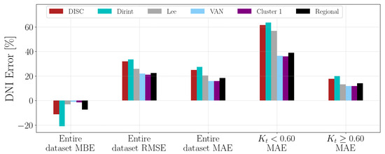
Figure A19. Hourly test results of decomposition model development for VAN.

Figure A19. Hourly test results of decomposition model development for VAN.

References

- Masters, G. Renewable and Efficient Electric Power Systems, 2nd ed.; John Wiley and Sons, Inc.: Hoboken, NJ, USA, 2013; pp. 186–245, 316–398. [Google Scholar]
- Sengupta, M.; Habte, A.; Wilbert, S.; Gueymard, C.; Remund, J. Best Practices Handbook for the Collection and Use of Solar Resource Data for Solar Energy Applications, 3rd ed.; NREL: Golden, CO, USA, 2021. [Google Scholar] [CrossRef]
- ISO 9060:2018; Solar Energy—Specification and Classification of Instruments for Measuring Hemispherical Solar and Direct Solar Radiation. ISO: Geneva, Switzerland, 2018.
- Lee, H.; Kim, S.Y.; Yun, C. Comparison of Solar Radiation Models to Estimate Direct Normal Irradiance for Korea. Energies 2017, 10, 594. [Google Scholar] [CrossRef]
- Bertrand, C.; Vanderveken, G.; Journée, M. Evaluation of decomposition models of various complexity to estimate the direct solar irradiance over Belgium. Renew. Energy 2015, 74, 618–626. [Google Scholar] [CrossRef]
- Liu, B.Y.; Jordan, R.C. The interrelationship and characteristic distribution of direct, diffuse and total solar radiation. Sol. Energy 1960, 4, 1–19. [Google Scholar] [CrossRef]
- Yang, D.; Gueymard, C.A. Ensemble model output statistics for the separation of direct and diffuse components from 1-min global irradiance. Sol. Energy 2020, 208, 591–603. [Google Scholar] [CrossRef]
- Boland, J.; Huang, J.; Ridley, B. Decomposing global solar radiation into its direct and diffuse components. Renew. Sustain. Energy Rev. 2013, 28, 749–756. [Google Scholar] [CrossRef]
- Ridley, B.; Boland, J.; Lauret, P. Modelling of diffuse solar fraction with multiple predictors. Renew. Energy 2010, 35, 478–483. [Google Scholar] [CrossRef]
- Soares, J.; Oliveira, A.P.; Božnar, M.Z.; Mlakar, P.; Escobedo, J.F.; Machado, A.J. Modeling hourly diffuse solar-radiation in the city of São Paulo using a neural-network technique. Appl. Energy 2004, 79, 201–214. [Google Scholar] [CrossRef]
- Talvitie, T.; Eldali, F.; Pinney, D. Predicting Solar Diffuse and Direct Components Using Deep Neural Networks. In Proceedings of the 2021 IEEE Power & Energy Society Innovative Smart Grid Technologies Conference (ISGT), Washington, DC, USA, 16–18 February 2021; pp. 1–5. [Google Scholar]
- Kalyanam, R.; Hoffmann, S. A Novel Approach to Enhance the Generalization Capability of the Hourly Solar Diffuse Horizontal Irradiance Models on Diverse Climates. Energies 2020, 13, 4868. [Google Scholar] [CrossRef]
- Bessafi, M.; Oree, V.; Khoodaruth, A.; Chabriat, J.P. Impact of decomposition and kriging models on the solar irradiance downscaling accuracy in regions with complex topography. Renew. Energy 2020, 162, 1992–2003. [Google Scholar] [CrossRef]
- Janjai, S.; Phaprom, P.; Wattan, R.; Masiri, I. Statistical models for estimating hourly diffuse solar radiation in different regions of Thailand. In Proceedings of the International Conference on Energy and Sustainable Development: Issues and Strategies (ESD 2010), Chiang Mai, Thailand, 2–4 June 2010; pp. 1–6. [Google Scholar] [CrossRef]
- Orgill, J.; Hollands, K. Correlation equation for hourly diffuse radiation on a horizontal surface. Sol. Energy 1977, 19, 357–359. [Google Scholar] [CrossRef]
- Erbs, D.; Klein, S.; Duffie, J. Estimation of the diffuse radiation fraction for hourly, daily and monthly-average global radiation. Sol. Energy 1982, 28, 293–302. [Google Scholar] [CrossRef]
- Louche, A.; Notton, G.; Poggi, P.; Simonnot, G. Correlations for direct normal and global horizontal irradiation on a French Mediterranean site. Sol. Energy 1991, 46, 261–266. [Google Scholar] [CrossRef]
- Maxwell, E. A Quasi-Physical Model for Converting Hourly Global Horizontal to Direct Normal Insolation; Technical Report; Solar Energy Research Institute: Golden, CO, USA, 1987. [Google Scholar]
- Perez, R.; Ineichen, P.; Maxwell, E.; Seals, R.; Zelenka, A. Dynamic global-to-direct irradiance conversion models. ASHRAE Trans. 1992, 98, 354–369. [Google Scholar]
- Lave, M.; Hayes, W.; Pohl, A.; Hansen, C.W. Evaluation of Global Horizontal Irradiance to Plane-of-Array Irradiance Models at Locations Across the United States. IEEE J. Photovoltaics 2015, 5, 597–606. [Google Scholar] [CrossRef]
- Lee, K.; Yoo, H.; Levermore, G.J. Quality control and estimation hourly solar irradiation on inclined surfaces in South Korea. Renew. Energy 2013, 57, 190–199. [Google Scholar] [CrossRef]
- Skartveit, A.; Olseth, J.A. A model for the diffuse fraction of hourly global radiation. Sol. Energy 1987, 38, 271–274. [Google Scholar] [CrossRef]
- Lam, J.C.; Li, D.H. Correlation between global solar radiation and its direct and diffuse components. Build. Environ. 1996, 31, 527–535. [Google Scholar] [CrossRef]
- Reindl, D.; Beckman, W.; Duffie, J. Diffuse Fraction Correlations. Sol. Energy 1990, 45, 1–7. [Google Scholar] [CrossRef]
- Yao, W.; Li, Z.; Xiu, T.; Lu, Y.; Li, X. New decomposition models to estimate hourly global solar radiation from the daily value. Sol. Energy 2015, 120, 87–99. [Google Scholar] [CrossRef]
- Khalil, S.A.; Shaffie, A. A comparative study of total, direct and diffuse solar irradiance by using different models on horizontal and inclined surfaces for Cairo, Egypt. Renew. Sustain. Energy Rev. 2013, 27, 853–863. [Google Scholar] [CrossRef]
- Gueymard, C.A.; Ruiz-Arias, J.A. Extensive worldwide validation and climate sensitivity analysis of direct irradiance predictions from 1-min global irradiance. Sol. Energy 2016, 128, 1–30. [Google Scholar] [CrossRef]
- Laiti, L.; Giovannini, L.; Zardi, D.; Belluardo, G.; Moser, D. Estimating Hourly Beam and Diffuse Solar Radiation in an Alpine Valley: A Critical Assessment of Decomposition Models. Atmosphere 2018, 9, 117. [Google Scholar] [CrossRef]
- Oliveira, A.P.; Escobedo, J.; Machado, A.; Soares, J. Correlation models of diffuse solar-radiation applied to the city of São Paulo, Brazil. Appl. Energy 2002, 71, 59–73. [Google Scholar] [CrossRef]
- Salazar, G.; Pedrosa Filho, M. Analysis of the Diffuse Fraction from Solar Radiation Values Measured in Argentina and Brazil Sites. In Proceedings of the Solar World Congress 2019, Santiago, Chile, 3–7 November 2020. [Google Scholar] [CrossRef]
- Chendo, M.; Maduekwe, A. Hourly global and diffuse radiation of Lagos, Nigeria—Correlation with some atmospheric parameters. Sol. Energy 1994, 52, 247–251. [Google Scholar] [CrossRef]
- Chikh, M.; Mahrane, A.; Haddadi, M. Modeling the Diffuse Part of the Global Solar Radiation in Algeria. Energy Procedia 2012, 18, 1068–1075. [Google Scholar] [CrossRef]
- Benchrifa, M.; Tadili, R.; Idrissi, A.; Essalhi, H.; Mechaqrane, A. Development of New Models for the Estimation of Hourly Components of Solar Radiation: Tests, Comparisons, and Application for the Generation of a Solar Database in Morocco. Int. J. Photoenergy 2021, 2021, 8897818. [Google Scholar] [CrossRef]
- Engerer, N. Minute resolution estimates of the diffuse fraction of global irradiance for southeastern Australia. Sol. Energy 2015, 116, 215–237. [Google Scholar] [CrossRef]
- Tsubo, M.; Walker, S. Relationships between photosynthetically active radiation and clearness index at Bloemfontein, South Africa. Theor. Appl. Climatol. 2005, 80, 17–25. [Google Scholar] [CrossRef]
- Nijegorodov, N. Improved ashrae model to predict hourly and daily solar radiation components in Botswana, Namibia, and Zimbabwe. Renew. Energy 1996, 9, 1270–1273. [Google Scholar] [CrossRef]
- Mabasa, B.; Lysko, M.D.; Tazvinga, H.; Zwane, N.; Moloi, S.J. The Performance Assessment of Six Global Horizontal Irradiance Clear Sky Models in Six Climatological Regions in South Africa. Energies 2021, 14, 2583. [Google Scholar] [CrossRef]
- Mahachi, T. Energy Yield Analysis and Evaluation of Solar Irradiance Models for a Utility Scale Solar PV Plant in South Africa. Master’s Thesis, University of Stellenbosch, Stellenbosch, South Africa, 2016. [Google Scholar]
- Daniel, F.M.; Rix, A.J. The Evaluation of Decomposition Models Under Varying Weather Conditions for South Africa. In Proceedings of the Southern African Sustainable Energy Conference, Stellenbosch, South Africa, 17–19 November 2021; pp. 207–213. [Google Scholar]
- Daniel-Durandt, F.M.; Rix, A.J. Automating Quality Control of Irradiance Data with a Comprehensive Analysis for Southern Africa. Solar 2023, 3, 596–617. [Google Scholar] [CrossRef]
- SAURAN. 2022. Available online: https://sauran.ac.za/ (accessed on 23 June 2022).
- Walpole, R.; Myers, R.; Myers, S.; Ye, K. Probability & Statistics for Engineers & Scientists; Pearson Education Inc.: Boston, MA, USA, 2012. [Google Scholar]
- Anaconda Software Distribution. 2020Anaconda Inc. Available online: https://www.anaconda.com/ (accessed on 14 February 2020).
- Holmgren, W.; Hansen, C.; Mikofski, M. pvlib python: A python package for modeling solar energy systems. J. Open Source Softw. 2018, 3, 884. [Google Scholar] [CrossRef]
- McKinney, W. Data structures for statistical computing in python. In Proceedings of the 9th Python in Science Conference, Austin, TX, USA, 28–30 June 2010; Volume 445, pp. 51–56. [Google Scholar]
- Hunter, J.D. Matplotlib: A 2D graphics environment. Comput. Sci. Eng. 2007, 9, 90–95. [Google Scholar] [CrossRef]
- Mahachi, T.; Rix, A. Evaluation of irradiance decomposition and transposition models for a region in South Africa Investigating the sensitivity of various diffuse radiation models. In Proceedings of the IECON 2016—42nd Annual Conference of the IEEE Industrial Electronics Society, Florence, Italy, 24–27 October 2016; pp. 3064–3069. [Google Scholar] [CrossRef]
- Kasten, F.; Young, A.T. Revised optical air mass tables and approximation formula. Appl. Opt. 1989, 28, 4735–4738. [Google Scholar] [CrossRef] [PubMed]
- Farmer, W.; Rix, A.J. Mapping the spatial perturbations seen by the power system network due to intermittent renewable energy sources. In Proceedings of the Southern African Sustainable Energy Conference, Stellenbosch, South Africa, 17–19 November 2021; pp. 222–228. [Google Scholar]
- GHI Solar Map ©2017 Solargis. 2021. Available online: https://solargis.com/maps-and-gis-data/download/south-africa (accessed on 27 July 2022).
Disclaimer/Publisher’s Note: The statements, opinions and data contained in all publications are solely those of the individual author(s) and contributor(s) and not of MDPI and/or the editor(s). MDPI and/or the editor(s) disclaim responsibility for any injury to people or property resulting from any ideas, methods, instructions or products referred to in the content. |
© 2024 by the authors. Licensee MDPI, Basel, Switzerland. This article is an open access article distributed under the terms and conditions of the Creative Commons Attribution (CC BY) license (https://creativecommons.org/licenses/by/4.0/).