Limits of Harmonic Stability Analysis for Commercially Available Single-Phase Inverters for Photovoltaic Applications

Abstract

The growth of renewables in public energy networks requires suitable strategies to assess the stable operation of the respective power electronic devices, e.g., inverters. Different assessment methods can be performed with regard to the available knowledge and the assessment objective, e.g., a specific frequency range or the input signal characteristics that are typically classified into small-signal and large-signal disturbances. This paper addresses the limits of the measurement-based small-signal stability analysis in the harmonic frequency range of commercially available single-phase inverters for photovoltaic applications. The harmonic stability is analyzed, and the results for a sinusoidal background voltage and distorted background voltages are assessed based on measurements. The measurements prove that even in the harmonic frequency range, the harmonic stability analysis can only provide a sufficient but not a necessary condition in terms of the statement towards an instable operation.

1. Introduction

The growth of renewables in public energy networks [1], e.g., low-voltage (LV) networks, leads to an increasing number of installed power electronic (PE) devices. One type of PE device is inverters that enable a DC-AC power conversion and connect DC power applications to AC networks. For low-power applications in public LV networks, these inverters are usually single-phase connected on the AC side.

To ensure the reliable operation of power grids, different approaches to model inverters and analyze their stability are known from the literature. Furthermore, the device emission of single-phase devices has to comply with respective standards, e.g., in Europe with the IEC 61000-3-2 [2], the IEC 61000-3-12 [3] and the IEC TS 61000-3-16 [4]. Despite precautionary studies, standards and regulations, the phenomenon of harmonic instabilities [5] has been reported in the field, i.e., firstly in the Swiss railway network [6]. Later, harmonic instabilities have also been measured and documented in distribution networks with large numbers of photovoltaic (PV) inverters, e.g., [7,8,9].

With regard to Power Quality analyses in the harmonic frequency range, i.e., above 50 Hz up to 2 kHz, white-box approaches can give detailed information about the origin of an instability but are only applicable if the topology and the parameters of the inverter are known, e.g., for device manufacturers. For commercially available inverters with unknown parameters, black-box approaches have been developed to measure the device characteristics and analyze the device stability afterwards.

The aim of this paper is the measurement-based demonstration of the limits of a black-box stability analysis in the harmonic frequency range. The measurements show that the black-box stability analysis based on the impedance-based stability criterion is not sufficient to reliably indicate the stable operation of an inverter.

In the following Section 2, the state of the art is introduced briefly. Section 3 presents the measurement setup and the measurement results of a commercially available single-phase inverter for PV applications. Section 4 discusses further aspects that are relevant for this topic, and finally, Section 5 concludes this study with a summary and refers to future work.

2. The State of the Art

The entire system can be modeled in two parts, i.e., the LV network and the inverter. A representation in frequency domain is depicted in Figure 1.

2.1. Low-Voltage Network Model

For harmonic studies, the LV network is typically represented by a network impedance Z_g and a voltage source. The network impedance reflects the linear voltage–current relation at the Point of Connection (PoC) and the voltage source the background voltage U_g to include the nonlinear characteristics, e.g., resulting from other grid-connected devices. Both the network impedance and the background voltage can vary largely depending on the type and number of grid-connected devices and the specifications of the network itself, e.g., length of cables and overhead lines, transformers, etc. For practical reasons and the lack of information, the network impedance is often simplified as an RL-equivalent that considers the X/R ratio at power system frequency.

2.2. Inverter Model

From a classical system modeling perspective, different types of models can be developed based on the available knowledge, e.g., the white-box, the gray-box and the black-box model.

2.2.1. White-Box Model

For white-box models, all (relevant) details of the device design have to be known. The most elaborate representation is the switched model that can accurately represent even multiples of the switching frequency. In general, but also for stability studies specifically, the appropriate solver settings are crucial for the accuracy of the simulation results and also affect the simulation duration significantly. To simplify the switched model and to reduce the computational effort, the switched model can be averaged and reduced to study-relevant components. A model that is suitable for most harmonic studies is the linear time-periodic (LTP) model in time domain with its general description in terms of

$$\dot{\mathit{x}}\left(t\right)=\mathit{A}\left(t\right)\mathit{x}\left(t\right)+\mathit{B}\left(t\right)\mathit{u}\left(t\right)$$

(1)

and

$$\mathit{y}\left(t\right)=\mathit{C}\left(t\right)\mathit{x}\left(t\right)+\mathit{D}\left(t\right)\mathit{u}\left(t\right).$$

(2)

The real-value system parameter matrices $\mathit{A}$, $\mathit{B}$, $\mathit{C}$ and $\mathit{D}$ are periodic with $T$, which is one cycle of the power system frequency f₁ in the form

$$\mathit{A}\left(t+T\right)=\mathit{A}\left(t\right)$$

(3)

The LTP model in time domain can be transferred into the harmonic state space (HSS) by Fourier expansion. The transferred model consists of harmonic transfer functions (HTFs) and can be arranged in a matrix in terms of

$$\mathit{H}\left(\mathrm{s}\right)=\left[\begin{array}{ccccc}\ddots & ⋮& ⋮& ⋮& \\ \dots & H_0\left(s-j{\omega }_1\right)& H_{-1}\left(s\right)& H_{-2}\left(s+j{\omega }_1\right)& \dots \\ \dots & H_1\left(s-j{\omega }_1\right)& H_0\left(s\right)& H_{-1}\left(s+j{\omega }_1\right)& \dots \\ \dots & H_2\left(s-j{\omega }_1\right)& H_1\left(s\right)& H_0\left(s+j{\omega }_1\right)& \dots \\ & ⋮& ⋮& ⋮& \ddots \end{array}\right]$$

(4)

White-box models are typically used by power electronic manufacturers and research institutions that design and analyze individual device components and parameters in detail.

2.2.2. Gray-Box Model

Gray-box modeling implies the availability of partial knowledge for the modeling process. Also, the identification of components in terms of the topology and individual parameters can be performed. While classical identification methods with regard to parameter estimation have been introduced long ago and the techniques are known, e.g., by using Kalman filter [10], recent approaches also include algorithms making use of artificial intelligence (AI), e.g., [11], to identify the parameters, e.g., gains of the control, of a known structure.

A second category that falls into gray-box approaches is the identification and parametrization of the subsystems, e.g., hardware components [12] of the inverter. Though equivalent models have been developed for different types of PE devices and some parametrization and component identification techniques have been proposed, holistic gray-box models for single-phase inverters are not known to the authors as of yet.

2.2.3. Black-Box Model

Typically, neither the topology nor the parameters of the topology of individual components of commercially available inverters are disclosed by the manufacturer. To develop black-box models, suitable identification methods have to be applied for their parametrization. Black models can be derived from white-box simulation models or from unknown inverters by measurements. For white-box models, it is possible to calculate the input–output signal characteristics of the internal design for each component and aggregate them into black-box models in the structure of (4), while the individual parameters such as L’s, C’s, R’s and the detailed terms of the controllers and the PLL, e.g., gains, filter-functions, etc., do not have to be disclosed but can be represented by numerical Eigenvalues. The calculated model is still subjected to the manufacturer tolerances of the individual physical components that can differ from the data sheet. On the other hand, unknown devices with an undisclosed design have to be identified by measurements in the laboratory.

While the first tests on the dynamic behavior of commercially available inverters, e.g., by step changes in the fundamental frequency and their transient reaction [13], have been conducted, no dynamic large-signal model is known to the authors. One of the constraints is that the model has to run in time domain to reflect the transient and instantaneous interaction on the AC side of the inverter. The Heisenberg–Gabor limit prevents the hybrid modeling of the inverter dynamics, i.e., modeling the interaction in combined frequency–time domain models. According to the Heisenberg–Gabor limit [14], the resolution of time ${\sigma }_t$ and frequency ${\sigma }_f$ is always constant with

$${\sigma }_t{\sigma }_f\ge {\displaystyle \frac{1}{4\mathsf{\pi }}}$$

(5)

Consequently, the time instance and the excited frequencies cannot both be identified at the moment of the occurrence of the transient.

Different black-box model structures have been tested and respective parametrization methods developed. With regard to time domain models, nonlinear models, e.g., neural networks [15] and the Hammerstein Wiener model ([16,17]), have been tested by using training and validation data with harmonic distortions. The technical limitations and possibilities have not been analyzed sufficiently, while the parametrization of these models also lacks a more detailed specification with regard to the test signals and the method’s application in general. However, these model structures present interesting approaches for black-box simulations of instabilities next to the analytic, classic stability analysis.

Since nonlinear, general black-box time domain models are currently not available, the state-of-the-art representation is the coupled Norton model, as depicted in Figure 1. The model is a small-signal model in frequency domain and is related to a reference point around which it is linearized. To identify the parameters of the coupled Norton model, measurements are performed in the laboratory.

2.2.4. Measurement-Based Identification

The measurement-based identification of LTP systems relies on the principle of a frequency sweep [18]. The application of the frequency sweep on PE devices in energy systems has been called the fingerprint [19]. In the first step, a reference voltage, e.g., a sinusoidal voltage at power system frequency, is applied at the AC-side inverter clamps for a specific power level. The current response ${\underset{\_}{I}}_{\mathrm{A}\mathrm{C} \mathrm{r}\mathrm{e}\mathrm{f}}\left(f_I\right)$ at all frequencies $f_I$ is measured for each measurement i. Next to a reference voltage ${\underset{\_}{U}}_{\mathrm{A}\mathrm{C} \mathrm{r}\mathrm{e}\mathrm{f}}\left(f_U\right)$, a single-frequent distortion is superimposed and swept over its frequency $f_U$ in terms of entire multiples of the power system frequency, i.e., the voltage harmonics. With regard to Figure 1, the current at the PoC can be expressed by the first Kirchhoff law (Kirchhoff’s Current Law) with

$${\underset{\_}{I}}_{\mathrm{P}\mathrm{o}\mathrm{C}}\left(f_I\right)={\underset{\_}{I}}_{\mathrm{P}\mathrm{o}\mathrm{C} \mathrm{r}\mathrm{e}\mathrm{f}}\left(f_I\right)+{\underset{\_}{U}}_{\mathrm{P}\mathrm{o}\mathrm{C}}\left(f_I\right)\underset{\_}{Y}\left(f_I\right)+\sum _{\begin{array}{c}{f}_U=0\\ f_U\ne f_I\end{array}}^{\mathrm{\infty }}\mathsf{\Delta }{\underset{\_}{U}}_{\mathrm{P}\mathrm{o}\mathrm{C}}\left(f_U\right){\underset{\_}{Y}}_{\mathrm{I}\mathrm{n}\mathrm{v}}(f_I,f_U).$$

(6)

The elements of the so-called frequency coupling matrix (FCM) Y, which was firstly introduced as a crossed frequency admittance matrix [20], at the specific power level can be calculated elementwise with

$${\underset{\_}{Y}}_{\mathrm{I}\mathrm{n}\mathrm{v}}\left(f_I,f_U\right)={\displaystyle \frac{{\underset{\_}{I}}_{\mathrm{P}\mathrm{o}\mathrm{C} i}\left(f_I\right)-{\underset{\_}{I}}_{\mathrm{P}\mathrm{o}\mathrm{C} \mathrm{r}\mathrm{e}\mathrm{f}}\left(f_I\right)}{{\underset{\_}{U}}_{\mathrm{P}\mathrm{o}\mathrm{C} i}\left(f_U\right)-{\underset{\_}{U}}_{\mathrm{P}\mathrm{o}\mathrm{C} \mathrm{r}\mathrm{e}\mathrm{f}}\left(f_U\right)}}.$$

(7)

The principle of the frequency sweep is generally applicable to LTP system representations. However, the linearity and the specifications with regard to the definition of the operating point (grid side and inverter side) are very individual for each type of PE device. For single-phase PV inverters, the voltage at the PoC (grid side) has an approximately linear impact on the current response, but the impact of the operating power (inverter side) needs to be considered separately by different sets of parameters [21].

2.3. Harmonic Stability Analysis

According to classical stability definition, e.g., [22], stability implies the ability of a system to remain in an equilibrium state under normal operating conditions and furthermore the convergence to an equilibrium state if subjected to disturbances. In general, stability is a system characteristic and relates to the entire frequency range. However, harmonic stability refers to the explicit interaction of harmonic voltages and currents at the PoC. This interaction is defined by the inverter control, the grid-side filter circuit and the network impedance. The harmonic stability analysis studies the frequency range above the power system frequency (e.g., 50 Hz in Europe) up to 2 kHz. Thus, the stability at power system frequency is not considered, e.g., the power balance between the consumer and generator and also active and reactive power as well as synchronization issues for large frequency and phase jumps due to the Phase-Locked Loop (PLL).

For the harmonic stability analysis, two main approaches are typically applied with regard to the available knowledge.

If a detailed inverter model is available, the Eigenvalue analysis, e.g., [23], according to Lyapunov is possible. The analysis is performed based on the time domain model and considers the detailed inverter design at a specific operating point, i.e., a specific operating power. For commercially available inverters, this is not suitable since the Eigenvalues are not disclosed.

Consequently, a second approach is applied for inverters with an unknown design, i.e., a black-box approach, called the impedance-based approach [24]. By applying the previously introduced frequency sweep either on a synthetic white-box model in simulations or on a physical device in the laboratory, the FCM and the respective impedance characteristics, i.e., the reciprocal of the main diagonal of the FCM, can be identified. By applying the Nyquist criterion on the impedance characteristics, the small-signal stability for a selected operating point, i.e., a specific operating power, can be analyzed. Previous work has demonstrated that the harmonic stability can be calculated for inverters with a known internal design, and the theory can be validated by measurements, e.g., [25]. The impedance-based calculation studies the ratio of the impedances as previously introduced. This method cannot consider the impact of harmonic (background) voltages at the PoC on the harmonic stability by definition of the stability and the system characteristics.

A constraint of both methods is that the impedance characteristics of the LV network have to be assumed. While typically, RL-equivalent circuits are considered for the network, Ref. [26] demonstrates that neglecting resonances by simply extrapolating the X/R ratio at power system frequency can lead to false conclusions towards the device stability. Therefore, a probabilistic approach by considering field measurements of LV network impedances has been applied exemplarily in [27].

3. Limits of Harmonic Stability Assessment

3.1. Theoretic Considerations

According to classical control theory, the device stability can be assessed as introduced previously. Though there are different definitions and approaches, it can be concluded that a stable system provides enough damping to decrease excited signals, while an instable system will increase the signal excitation. To provide stable operation, this is not sufficient, which will be demonstrated in the following. It seems obvious that strong signal excitations will trigger overcurrent and overvoltage protections within the device even in the absence of an impedance connected to the AC side of the inverter. This unwanted behavior is called tripping. For a statement towards the stable operation of the inverter, both the tripping and the stability have to be considered. Eventually, they will both challenge the device immunity. Currently, measurement-based assessments consider only the device stability and neglect the impact of the background distortion. From the stability point of view, the distortion of the background voltage provides a disturbance to the system. If the system is stable, the system is able to handle the distortion, i.e., the distortion at the PoC remains stable and is not amplified. Consequently, the background distortion is neglected in the stability analysis as it does not affect the stability of the system.

In [28], a so-called flat-top voltage has been identified that represents the typical voltage waveform at a PoC in public LV networks in western Europe. The flat-top waveform [29] voltage meets the distortion limits specified by the relevant standards, e.g., the EN 50160 [30] or the IEC 61000-2-2 [31]. The spectrum of this flat-top voltage according to [28] will be used as representative background voltage later in this study.

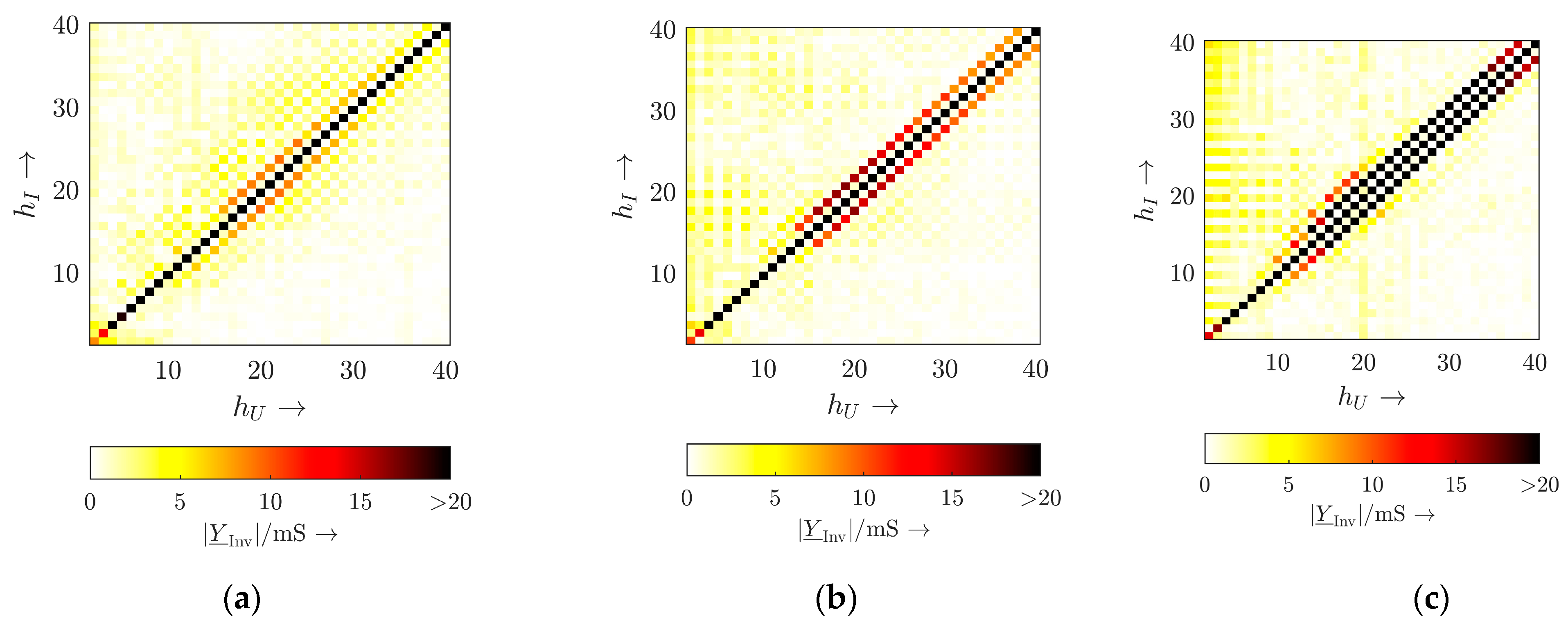
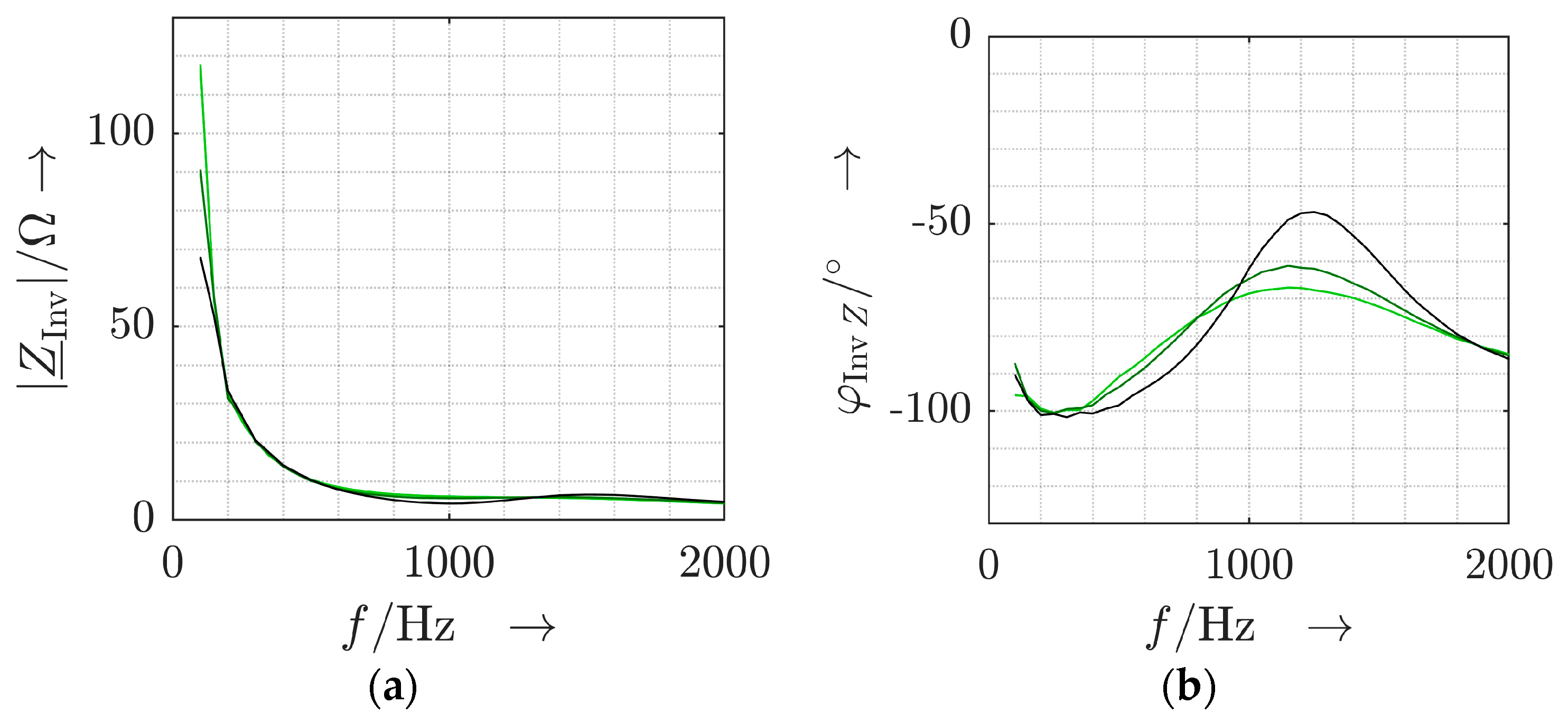
3.2. Measurement-Based Identification of Small-Signal Characteristics

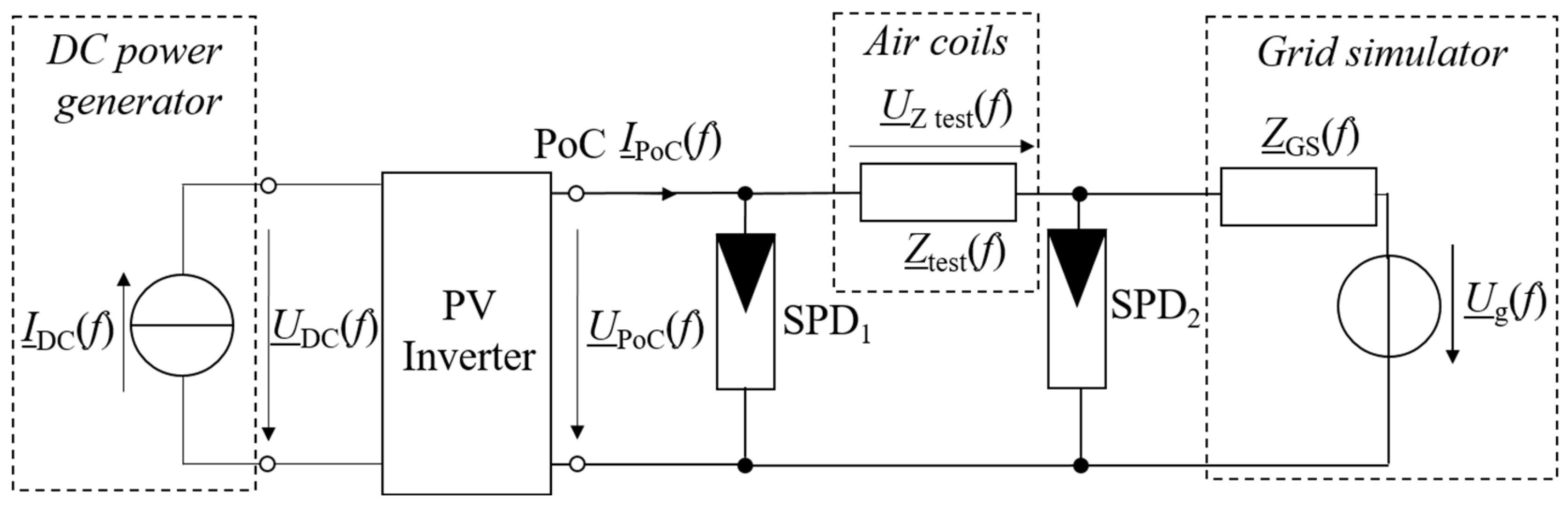
3.2.1. Measurement Setup

The test stand consists of a network simulator that provides the AC-side background voltage and is rated at 45 kVA. The measured, commercially available single-phase inverter for PV applications is rated at 4.5 kW which represents a typical inverter for PV rooftop applications as typical power ratings of single-phase inverters for PV rooftop applications are between 2.0 kW and 4.6 kW. The power on the DC side of the inverter is provided by a DC power generator rated at 7 kW that is controlled by a software to emulate the characteristics of solar panels and the respective strings. This software also includes the possibility to set a voltage–current characteristic with a Maximum Power Point (MPP) of the solar panel operation that is set to 400 V as the optimum DC-link voltage in this study. The Maximum Power Point Tracker (MPPT) of the inverter tracks the change in the voltage–current characteristics to enable the optimal operation of the solar panels.

For identifying the small-signal characteristics of the inverter, no extra impedance is implemented, i.e., the impedance of the test stand seen by the inverter at the PoC is as low as possible, ideally zero.

The maximum acceptable measurement uncertainty has been defined with 10% by the authors and can be ensured for voltage amplitudes above 20 mV and current amplitudes above 20 mA. The sampling rate of the transient recorder is set to 1 MS/s.

To identify the small-signal characteristics, i.e., the FCMs and impedances of the inverter at different operating points, the frequency sweep as described in Section 2.2.4 is applied. The parameters of the sweep component for the frequency sweep have been set to an amplitude of $5\sqrt{2}$ V with a phase angle of 0°. The amplitude of the sweep component has to be large enough to be dominant with respect to measurement uncertainties and noise but low enough to comply with the limits of the maximum voltage distortion at the PoC to enable the stable operation of the inverter.

3.2.2. Measurement Results

The magnitudes of the FCMs for the three operating points, i.e., 1 kW, 2.5 kW and 4.5 kW, are depicted as heatmaps in Figure 2.

For the impedance-based stability analysis, the impedance characteristics of the inverter are required (phase angle and magnitude). They correspond to the inverse of the diagonal elements of the FCMs and can be calculated in complex domain with

$$\underset{\_}{Z}\left(f\right)={\displaystyle \frac{1}{{\underset{\_}{Y}}_{\mathrm{I}\mathrm{n}\mathrm{v}}(f_I,f_U)}}\forall f_I=f_U=f.$$

(8)

The results are depicted in Figure 3 and demonstrate the dependency of magnitude and phase angle characteristics on the operating power.

3.3. Measurement-Based Evaluation of Stable Operation

3.3.1. Measurement Setup

Test Stand Configuration

For measuring the inverter under non-ideal conditions, specifically with regard to the later superposition of distorted background voltages and the presence of an impedance, the test stand and the respective measurement setup are depicted in Figure 4.

For setting a large range of inductance values, air coils are used to form the test impedance Z_test. The implementation provides a cost-efficient and flexible setup and has been introduced in [32]. The individual inductance value of each air coil is between 1 mH and 1.3 mH. The air coils are physically arranged in pairs. Each pair of air coils consists of two air coils wound into each other that can be connected in series or parallel. By arranging multiple pairs of air coils, the air gap between coils of different pairs can be varied to adjust the resulting inductance. The resulting inductance L_test is determined by the respective inductance values L₁ and L₂ and the air gap in terms of the magnetic coupling M with

$$L_{\mathrm{t}\mathrm{e}\mathrm{s}\mathrm{t}}=L_1+L_2+2M$$

(9)

Any adjusted inductance values of Z_test (cf.

Table 1. Measurement results for sinusoidal and flat-top reference voltage.

Operating Power	Inductance Value @1 kHz	Operation Status
		Sinusoidal Voltage	Flat-Top Voltage (and Pointed-Top)
1 kW	3785 µH	Stable	Stable
	3943 µH	Stable	Instable
	4112 µH	Instable	-
2.5 kW	3785 µH	Stable	Stable
	3943 µH	Instable	-
	4112 µH	Instable	-
4.5 kW	1625 µH	Stable	Stable
	1908 µH	Stable	Instable
	2385 µH	Instable	-

) have been verified at 1 kHz by using an LCR measurement bridge.

Measurement Scenarios

For each operating power, critical inductance values are determined according to the impedance-based stability criterion. With regard to real measurements as performed in the following, a range of inductance values around the theoretic values are set via the air coils to consider parasitic effects and uncertainties in the measurements. The applied inductance values are listed in Table 1 together with the measured operating status of the inverter. These critical impedances are higher than realistic values in public LV networks, as the main purpose of this study is the analysis of the limits of the stable operation of the inverter in the harmonic range.

The background voltage is set as sinusoidal, flat-top and also pointed-top waveform. While the flat-top voltage waveform is typical for public LV networks, the pointed-top voltage waveform is rather representative for industry LV networks. In case the flat-top voltage waveform caused an instable operation of the inverter, the pointed-top voltage waveform was not applied, as the flat-top voltage waveform already indicated the impact of a background voltage distortion. As a result, the pointed-top voltage waveform was only measured for stable inverter operations and did not cause additional instable inverter operations. Instable implies, in this study, that the inverter shuts down. An overview of the test measurements is listed in Table 1.

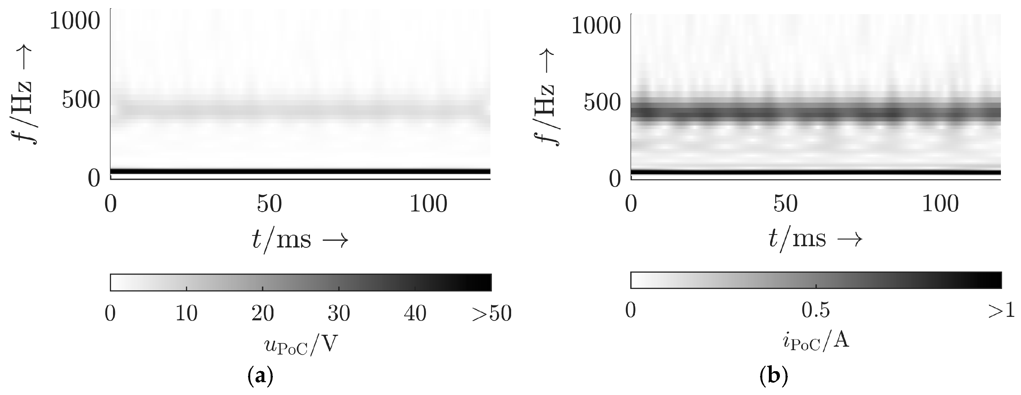
3.3.2. Measurement Results

The measurement results have been plotted exemplarily for 1 kW for undistorted (sinusoidal) background voltage (Figure 5 and Figure 6) and distorted (flat-top) voltage (Figure 7 and Figure 8) for the scenario where the inverter is operating stable with sinusoidal background voltage but is not able to operate stable and shuts down for the flat-top background voltage, i.e., with a test stand inductance L_test of 3.943 mH.

3.3.3. Measurement Result Categorization

For the individual measurements, different results can be identified with regard to the general stability statement, i.e., stable or instable, and, in the case of an instability, furthermore specified into the type of instability, i.e., if the device shuts down during steady state (category 2A), if the device shuts down during the change in the voltage waveform of the background voltage (category 2B) or if the device was not able to reach the intended operating point, which is called unspecified (category 2C). An overview of this classification is presented in

Table 2. Categories of measured results.

Cate-Gory		Stability Statement	Type of Instability	Voltage Waveform	Specifications
1		Stable	-	Sinusoidal	-
				Flat-top	-
				Pointed-top	-
2	A	Instable	Steady state	Sinusoidal	-
				Flat-top	-
	B	Instable	Transient	Sinusoidal to flat-top	Shut down when changing the background voltage
	C	Instable	Unspecified	Sinusoidal	Not reaching the intended operating point before shutting down

.

3.3.4. Measurement Evaluation

Stable inverter operations (category 1) have been measured in addition to the presented measurements for selected test impedance values below the listed values in Table 1 for the specific power levels for the three voltage waveforms and been presented by the authors in [21]. These measurements have not been listed separately as they all indicated a stable inverter operation as expected.

For the assessment of the steady-state stability (category 2A) with a sinusoidal background voltage, the operation at different operating power demonstrates that impedance-based stability can provide a reasonable statement for one operating power though a general stability assessment requires the analysis of a suitable set of different operating powers.

The background distortion, here tested with the flat-top voltage waveform, has an impact on the stable operation for an intended steady state (category 2A). The measurements indicate that the distorted background voltage causes the inverter to shut down, before the impedance-based analysis, i.e., by the Nyquist criterion, concludes a shut down. This is different from simply assuming a certain phase margin reserve due to inaccuracies and swinging since the operation with sinusoidal reference voltage can be related rather accurately to the prediction based on the Nyquist criterion.

The transient stability is challenged when changing the background voltage (category 2B) for setups where the impedance-based criterion indicates a low stability margin, i.e., the phase margin and the reserve before the inverter becomes instable are small. This indicates that the system is not dampened sufficiently. The transient voltage u_PoC triggers a transient response of the inverter current i_PoC and accounts a broadband excitation, depending on the point on wave (PoW) at which the voltage amplitudes are changed or the size of the phase angle step change. For category 2B, the Nyquist criterion can give a first indication, but specifically, resonances in the network impedance and frequency-specific immunity of the inverter can challenge the prediction.

For strongly distorted voltages at the PoC, e.g., due to the interaction of the inverter current with the test stand impedance, the inverter is not even able to reach its steady-state operating point (category 2C). The attempts to reach the intended operating power, e.g., by the MPPT, can be interrupted immediately as soon as the DC power is present, or it can take over a minute before the inverter shuts down eventually. Since the inverter has not reached an equilibrium point, this category is neither related to steady-state stability nor transient stability.

4. Discussion

4.1. Network Impedance

In accordance with typical state-of-the-art analysis approaches, only RL-equivalent test impedances have been used in this study. It is a challenge to consider the possible frequency-dependent network impedances of real public LV networks in the measurement setup due to their multiple degrees of freedom, e.g., resonances (magnitude and phase angle characteristics). For one, this is because of the large range of magnitudes and phase angles in terms of their absolute values but also in terms of their frequency dependency, e.g., the change in one network impedance over its frequency spectrum. Secondly, it is a challenge to build impedances that allow for setting and adjusting resonances within the test impedance from the physical perspective with regard to power ratings of some kW.

However, for the identification of the stable operation in a specific frequency range, only the frequency-dependent values of the impedances, i.e., inverter and network, matter but not the physical implementation. Thus, the measurement results will be similar for measurements based on RL-equivalents and other designs (T-equivalent, $\pi$-equivalent, etc.) if the impedance values in the critical frequency region are similar.

4.2. Background Distortion

One of the main outcomes of this study is the impact of the background distortion on the stable operation of the inverter. While the impact of the network impedance on the inverter stability can be analyzed, the classical assumption towards the background distortion is that it does not affect the stability of the inverter or is simply neglected. If the voltage distortion at the PoC depends solely on the interaction of the current injected by the inverter and the network impedance, i.e., the background voltage distortion is zero, the voltage distortion is considered by the impedance-based analysis. However, next to linear voltage–current relations at the PoC, there are also effects that superimpose nonlinear voltage–current relations. Independent voltage emissions, e.g., due to fixed switching frequencies of pulse-width modulated (PWM)-based grid-connected power electronic devices, rectifiers and simply nonlinear hardware characteristics (semiconductors, non-ideal inductances, capacitances, etc.) are not considered in the impedance-based stability. Since they are independent, they will not violate the stability by its classical definition in terms of amplifications or damping as they only introduce an independent disturbance to the system. However, stable operation is not only related to classical stability phenomena but includes all effects that challenge the device immunity.

4.3. General Assessment Framework

Nowadays, for single-phase PV inverters in the frequency range up to 2 kHz, only current emission limits measured at sinusoidal supply voltage and without network impedance according to the newly developed IEC 61000-3-16 [4] apply. With regard to immunity, IEC 61000-4-13 [29] specifies tests with individual harmonic voltages and combinations of harmonic voltages (flat-top, pointed-top).

As this study proves that the reliable operation of single-phase PV inverters, i.e., stable operation, includes not only the interaction between inverters and the network impedance but also the resilience towards an existing voltage distortion and voltage transients at the PoC, the device testing according to present regulations and standards should be reconsidered. Recent laboratory measurements made by the authors have demonstrated the differences in the device emission between different inverter designs from different manufacturers for sinusoidal voltage but also in terms of their response to distorted voltages (steady state) and voltage transients [13]. Consequently, testing methods should include a typical range of voltage distortion levels and suitable voltage waveforms [33].

With regard to the device immunity, more advanced test methods including different operating powers and the superposition of the test stand impedance and the background voltage are required. A frequency-dependent sensitivity index has to be developed in general to assess individual inverter designs towards their grid robustness. The first test measurements in the laboratory have shown a higher sensitivity of individual inverters on low even-order harmonics compared to others in the frequency range up to about 300 Hz.

5. Conclusions

5.1. Summary

This paper demonstrates that the currently applied black-box small-signal stability analysis is bound to classical stability analysis. Though the impedance-based stability criterion according to Nyquist indicated the stable operation of the inverter, the introduction of a background distortion in the supply voltage that presents a typical voltage waveform in public LV networks caused the inverter to shut down. An overall statement towards the stable operation, even restricted to the harmonic frequency range and considering only reasonable background distortions, cannot be generally concluded. Harmonic stability as the current state of the art consequently represents a relevant part but does not holistically cover the immunity assessment in the harmonic frequency range. If the impedance-based analysis concludes an instable inverter operation, the statement is sufficient. However, the impedance-based analysis cannot give a statement towards the stable operation of the inverter in reverse, since the background distortion can exceed the immunity limits and cause a shut down.

5.2. Future Work

This study demonstrates the necessity to develop a holistic immunity framework that includes not only the classical stability analysis but also the superposition of the background distortion and the network impedance. Though the detailed white-box analysis would be able to perform such an analysis, a measurement-based framework is missing for the analysis and assessment of commercially available devices including PV inverters with an unknown topology. This framework should include more realistic testing conditions, e.g., typical network impedance characteristics including possible resonance conditions, a comprehensive set of different background distortions which could be based on probabilistic approaches based on grid measurement campaigns as well as testing transient voltages.

Furthermore, an emission framework and appropriate contribution assessment techniques should be developed with regard to the impact of the current emission on other grid-connected devices. To enable these tests, an adjustable test stand impedance for power ratings of some kW will have to be designed and implemented.

References

1. REN21 Renewables 2022 Global Status Report 2022. Available online: https://www.ren21.net/wp-content/uploads/2019/05/GSR2022_Full_Report.pdf (accessed on 14 July 2024).
2. IEC 61000-3-2:2018; Electromagnetic Compatibility (EMC)—Part 3-2: Limits—Limits for Harmonic Current Emissions (Equipment Input Current ≤ 16 A per Phase). IEC: Geneva, Switzerland, 2018.
3. IEC 61000-3-12:2011; Electromagnetic Compatibility (EMC)—Part 3-12: Limits—Limits for Harmonic Currents Produced by Equipment Connected to Public Low-Voltage Systems with Input Current > 16 A and ≤ 75 A per Phase. IEC: Geneva, Switzerland, 2011.
4. IEC TS 61000-3-16:2023; Electromagnetic Compatibility (EMC)-Part 3-16: Limits—Limits for Harmonic Currents Produced by the Inverter of Inverter-Type Electrical Energy-Supplying Equipment, with a Reference Current Less than or Equal to 75 A per Phase. IEC: Geneva, Switzerland, 2023.
5. Wang, X.; Blaabjerg, F. Harmonic Stability in Power Electronic-Based Power Systems: Concept, Modeling, and Analysis. IEEE Trans. Smart Grid 2019, 10, 2858–2870. [Google Scholar] [CrossRef]
6. Möllerstedt, E.; Bernhardsson, B. Out of Control Because of Harmonics-an Analysis of the Harmonic Response of an Inverter Locomotive. IEEE Control Syst. 2000, 20, 70–81. [Google Scholar] [CrossRef]
7. Enslin, J.H.R.; Heskes, P.J.M. Harmonic Interaction Between a Large Number of Distributed Power Inverters and the Distribution Network. IEEE Trans. Power Electron. 2004, 19, 1586–1593. [Google Scholar] [CrossRef]
8. Höckel, M.; Gut, A.; Arnal, M.; Schild, R.; Steinmann, P.; Schori, S. Measurement of Voltage Instabilities Caused by Inverters in Weak Grids. CIRED-Open Access Proc. J. 2017, 2017, 770–774. [Google Scholar] [CrossRef]
9. Moghbel, M.; Glenister, S.; Calais, M.; Shahnia, F.; Carter, C.; Edwards, D.; Stephens, D.; Jones, L.; Trinkl, P. Fluctuations in the Output Power of Photovoltaic Systems Distributed Across a Town with an Isolated Power System Using High-Resolution Data. In Proceedings of the 2019 9th International Conference on Power and Energy Systems (ICPES), Perth, Australia, 10–12 December 2019; pp. 1–5. [Google Scholar]
10. Kalman, R.E. A New Approach to Linear Filtering and Prediction Problems. J. Basic Eng. 1960, 82, 35–45. [Google Scholar] [CrossRef]
11. Lin, B.H.; Tsai, J.T.; Lian, K.L. A Non-Invasive Method for Estimating Circuit and Control Parameters of Voltage Source Converters. IEEE Trans. Circuits Syst. I Regul. Pap. 2019, 66, 4911–4921. [Google Scholar] [CrossRef]
12. Kaufhold, E.; Meyer, J.; Schegner, P. Black-Box Identification of Grid-Side Filter Circuit for Improved Modelling of Single-Phase Power Electronic Devices for Harmonic Studies. Electr. Power Syst. Res. 2021, 199, 107421. [Google Scholar] [CrossRef]
13. Kaufhold, E.; Meyer, J.; Schegner, P. Transient Response of Single-Phase Photovoltaic Inverters to Step Changes in Supply Voltage Distortion. In Proceedings of the 2020 19th International Conference on Harmonics and Quality of Power (ICHQP), Dubai, United Arab Emirates, 6–7 July 2020; IEEE: Dubai, United Arab Emirates, 2020; pp. 1–6. [Google Scholar]
14. Gabor, D. Theory of Communication. Part 1: The Analysis of Information. J. Inst. Electr. Eng.-Part III Radio Commun. Eng. 1946, 93, 429–441. [Google Scholar] [CrossRef]
15. Kaufhold, E.; Grandl, S.; Meyer, J.; Schegner, P. Feasibility of Black-Box Time Domain Modeling of Single-Phase Photovoltaic Inverters Using Artificial Neural Networks. Energies 2021, 14, 2118. [Google Scholar] [CrossRef]
16. Patcharaprakiti, N.; Kirtikara, K.; Chenvidhya, D.; Monyakul, V.; Muenpinij, B. Modeling of Single Phase Inverter of Photovoltaic System Using System Identification. In Proceedings of the 2010 Second International Conference on Computer and Network Technology, Bangkok, Thailand, 23–25 April 2010; pp. 462–466. [Google Scholar]
17. Wiesermann, L.M. Developing a Transient Photovoltaic Inverter Model in Opendss Using the Hammerstein-Wiener Mathematical Structure. Ph.D. Thesis, University of Pittsburgh, Pittsburgh, PA, USA, 2017. [Google Scholar]
18. Hall, S.R.; Wereley, N.M. Generalized Nyquist Stability Criterion for Linear Time Periodic Systems. In Proceedings of the 1990 American Control Conference, San Diego, CA, USA, 23–25 May 1990; pp. 1518–1525. [Google Scholar]
19. Cobben, S.; Kling, W.; Myrzik, J. The Making and Purpose of Harmonic Fingerprints. In Proceedings of the 19th International Conference on Electricity Distribution, Vienna, Austria, 21–24 May 2007; pp. 21–24. [Google Scholar]
20. Fauri, M. Harmonic Modelling of Non-Linear Load by Means of Crossed Frequency Admittance Matrix. IEEE Trans. Power Syst. 1997, 12, 1632–1638. [Google Scholar] [CrossRef]
21. Kaufhold, E.; Meyer, J.; Myrzik, J.; Schegner, P. Harmonic Stability Assessment of Commercially Available Single-Phase Photovoltaic Inverters Considering Operating-Point Dependencies. Solar 2023, 3, 473–486. [Google Scholar] [CrossRef]
22. Kundur, P. Power System Stability and Control; McGraw-Hill, Inc.: New York, NY, USA, 1994; p. 1176. [Google Scholar]
23. Salis, V.; Costabeber, A.; Cox, S.M.; Zanchetta, P. Stability Assessment of Power-Converter-Based AC Systems by LTP Theory: Eigenvalue Analysis and Harmonic Impedance Estimation. IEEE J. Emerg. Sel. Top. Power Electron. 2017, 5, 1513–1525. [Google Scholar] [CrossRef]
24. Sun, J. Impedance-Based Stability Criterion for Grid-Connected Inverters. IEEE Trans. Power Electron. 2011, 26, 3075–3078. [Google Scholar] [CrossRef]
25. Salis, V.; Costabeber, A.; Cox, S.M.; Tardelli, F.; Zanchetta, P. Experimental Validation of Harmonic Impedance Measurement and LTP Nyquist Criterion for Stability Analysis in Power Converter Networks. IEEE Trans. Power Electron. 2019, 34, 7972–7982. [Google Scholar] [CrossRef]
26. Kaufhold, E.; Meyer, J.; Schegner, P. Impact of Grid Impedance and Their Resonance on the Stability of Single-Phase PV-Inverters in Low Voltage Grids. In Proceedings of the 2020 IEEE 29th International Symposium on Industrial Electronics (ISIE), Delft, The Netherlands, 17–19 June 2020; pp. 880–885. [Google Scholar]
27. Kaufhold, E.; Meyer, J.; Müller, S.; Schegner, P. Probabilistic Stability Analysis for Commercial Low Power Inverters Based on Measured Grid Impedances. In Proceedings of the 2019 9th International Conference on Power and Energy Systems (ICPES), Perth, Australia, 10–12 December 2019; pp. 1–6. [Google Scholar]
28. Langella, R.; Testa, A.; Meyer, J.; Moller, F.; Stiegler, R.; Djokic, S.Z. Experimental-Based Evaluation of PV Inverter Harmonic and Interharmonic Distortion Due to Different Operating Conditions. IEEE Trans. Instrum. Meas. 2016, 65, 2221–2233. [Google Scholar] [CrossRef]
29. IEC 61000-4-13:2002; Electromagnetic Compatibility (EMC)—Part 4-13: Testing and Measurement Techniques—Harmonics and Interharmonics Including Mains Signalling at a.c. Power Port, Low Frequency Immunity Tests. IEC: Geneva, Switzerland, 2002.
30. EN 50160:2022; Voltage Characteristics of Electricity Supplied by Public Electricity Networks. Cenelec: Brussels, Belgium, 2022.
31. IEC 61000-2-2:2002; Electromagnetic Compatibility (EMC)—Part 2-2: Einvironment—Compatibility Levels for Low-Frequency Conducted Disturbances and Signalling in Public Low-Voltage Power Supply Systems. IEC: Geneva, Switzerland, 2002.
32. Kaufhold, E.; Duque, C.A.; Meyer, J.; Schegner, P. Measurement-Based Black-Box Harmonic Stability Assessment of Single-Phase Power Electronic Devices Based on Air Coils. IEEE Trans. Instrum. Meas. 2022, 71, 1–9. [Google Scholar] [CrossRef]
33. Kaufhold, E.; Meyer, J.; Myrzik, J.; Schegner, P. Framework to Assess the Stable Operation of Commercially Available Single-Phase Inverters for Photovoltaic Applications in Public Low Voltage Networks. Renew. Energy Power Qual. J. 2023, 21, 214–219. [Google Scholar] [CrossRef]
Figure 1. A frequency domain model of a PV inverter (coupled Norton model) and a public LV network (Thevenin equivalent).
Solar 04 00017 g001
Figure 2. Heatmaps of magnitudes of frequency coupling matrices for 1 kW (a), 2.5 kW (b) and 4.5 kW (c).
Solar 04 00017 g002
Figure 3. Magnitude (a) and phase angle (b) characteristics of the inverter for 1 kW (light green), 2.5 kW (dark green) and 4.5 kW (black).
Solar 04 00017 g003
Figure 4. A scheme of the test stand configuration for evaluating the stable operation of an inverter.
Solar 04 00017 g004
Figure 5. Voltage u P o C (a) and current i P o C (b) of inverter at 1 kW in time domain for sinusoidal background voltage and applied test stand impedance Ltest of 3.943 mH.
Solar 04 00017 g005
Figure 6. Voltage u P o C (a) and current i P o C (b) of inverter at 1 kW in wavelet domain for sinusoidal background voltage and applied test stand impedance Ltest of 3.943 mH.
Solar 04 00017 g006
Figure 7. Voltage u P o C (a) and current i P o C (b) during shut down of inverter at 1 kW in time domain for flat-top background voltage and applied test stand impedance Ltest of 3.943 mH.
Solar 04 00017 g007
Figure 8. Voltage u P o C (a) and current i P o C (b) during shut down of inverter at 1 kW in wavelet domain for flat-top background voltage and applied test stand impedance Ltest of 3.943 mH.
Solar 04 00017 g008