Blade-Resolved CFD Simulations of a Periodic Array of NREL 5 MW Rotors with and without Towers

Abstract

A fully resolved (FR) NREL 5 MW turbine model is employed in two unsteady Reynolds-averaged Navier–Stokes (URANS) simulations (one with and one without the turbine tower) of a periodic atmospheric boundary layer (ABL) to study the performance of an infinitely large wind farm. The results show that the power reduction due to the tower drag is about 5% under the assumption that the driving force of the ABL is unchanged. Two additional simulations using an actuator disc (AD) model are also conducted. The AD and FR results show nearly identical tower-induced reductions of the wind speed above the wind farm, supporting the argument that the AD model is sufficient to predict the wind farm blockage effect. We also investigate the feasibility of performing delayed-detached-eddy simulations (DDES) using the same FR turbine model and periodic domain setup. The results show complex turbulent flow characteristics within the farm, such as the interaction of large-scale hairpin-like vortices with smaller-scale blade-tip vortices. The computational cost of the DDES required for a given number of rotor revolutions is found to be similar to the corresponding URANS simulation, but the sampling period required to obtain meaningful time-averaged results seems much longer due to the existence of long-timescale fluctuations.

1. Introduction

A variety of approaches exist to model wind turbines of different sizes and types, for different purposes of use. Each type of model has its specific strengths and weaknesses. The actuator disc (AD) model has been widely adopted in wind energy studies [1,2,3,4] as it is relatively simple to implement and has low computational cost; however, it can represent only limited details of the turbine. The actuator line (AL) model considers the rotational motion of turbine blades and uses predetermined aerofoil data to represent the loading on each blade [5,6,7] with a medium computational cost. The most comprehensive and computationally intensive method is the fully resolved (FR) model, where the exact 3D geometry of the wind turbine is resolved during simulations; therefore, it models turbine motions and flow behaviours in a much more realistic manner [8,9,10].

Due to the complex and computationally expensive nature of the FR turbine model, it has been primarily used for simulations of an isolated turbine or a very small number (commonly two) of turbines [11,12,13,14], not for large wind farm cases. In addition, although the turbine tower is commonly present in FR turbine models, the tower effects on the efficiency of turbines or a wind farm are rarely discussed in detail.

In 2009, Zahle et al. [15] conducted investigations on wind turbine rotor–tower interaction using an FR NREL Phase VI turbine model [16]. Two simulations (using EllipSys3D) were presented in their study: one for an isolated rotor and the other for a downwind configuration of a full turbine (with tower) under tunnel flow conditions. The results of the simulations showed good agreement with existing experimental data. The CFD data showed a clear interaction between the tower wake and rotor blades, which caused noticeable velocity deficit in the wake, and the blades had a strong effect on the tower shedding frequency. However, there was no discussion on how the tower affects the turbine efficiency in this study.

In a more recent study, Rodrigues and Lengsfeld [9,17] developed a twin FR turbine model (parallel configuration) based on the MEXICO (Model Experiments in Controlled Conditions) experiment [18] to investigate the performance of a turbine in a wind farm. Their approach to mimic wind farm flow conditions was to perform sequential simulations, where the outlet of one simulation (for the first row of turbines in a wind farm) was used as the inlet of the other simulation (for the second row of turbines). The results showed clear tower wakes in both near- and far-wake flow fields. Noticeable velocity deficit and increased turbulence intensity caused by the turbine towers were also reported. Their approach of modelling wind farm flow has the advantage of not having to deploy multiple rows of turbines in the domain, dramatically reducing the mesh size and, hence, simulation cost. However, the wind farm layout investigated was limited to fully aligned and 10D spacing between each row of turbines, which are less commonly seen in modern large wind farms.

As a continuation of a recent study by Delafin and Nishino [19], in this paper, we employ an FR turbine model in a horizontally periodic computational domain to investigate the performance of an infinitely large wind farm with a fully staggered layout, with and without the turbine towers. The FR turbine model is based on the NREL 5 MW horizontal-axis turbine design [20,21], and the wind flow is simulated by solving the unsteady Reynolds-averaged Navier–Stokes (URANS) equations. A fully developed wind farm boundary layer is achieved by applying periodic boundary conditions, which enable the simulation of a single turbine to represent a turbine operating inside an infinitely large wind farm. The FR-URANS results are compared with corresponding AD-RANS results, as well as a theoretical model based on the two-scale momentum theory [22,23]. In addition, we also perform a delayed-detached-eddy simulation (DDES) using the same FR turbine model, to demonstrate the possibility of eddy-resolving FR turbine simulations for wind farm modelling.

2. Methodology

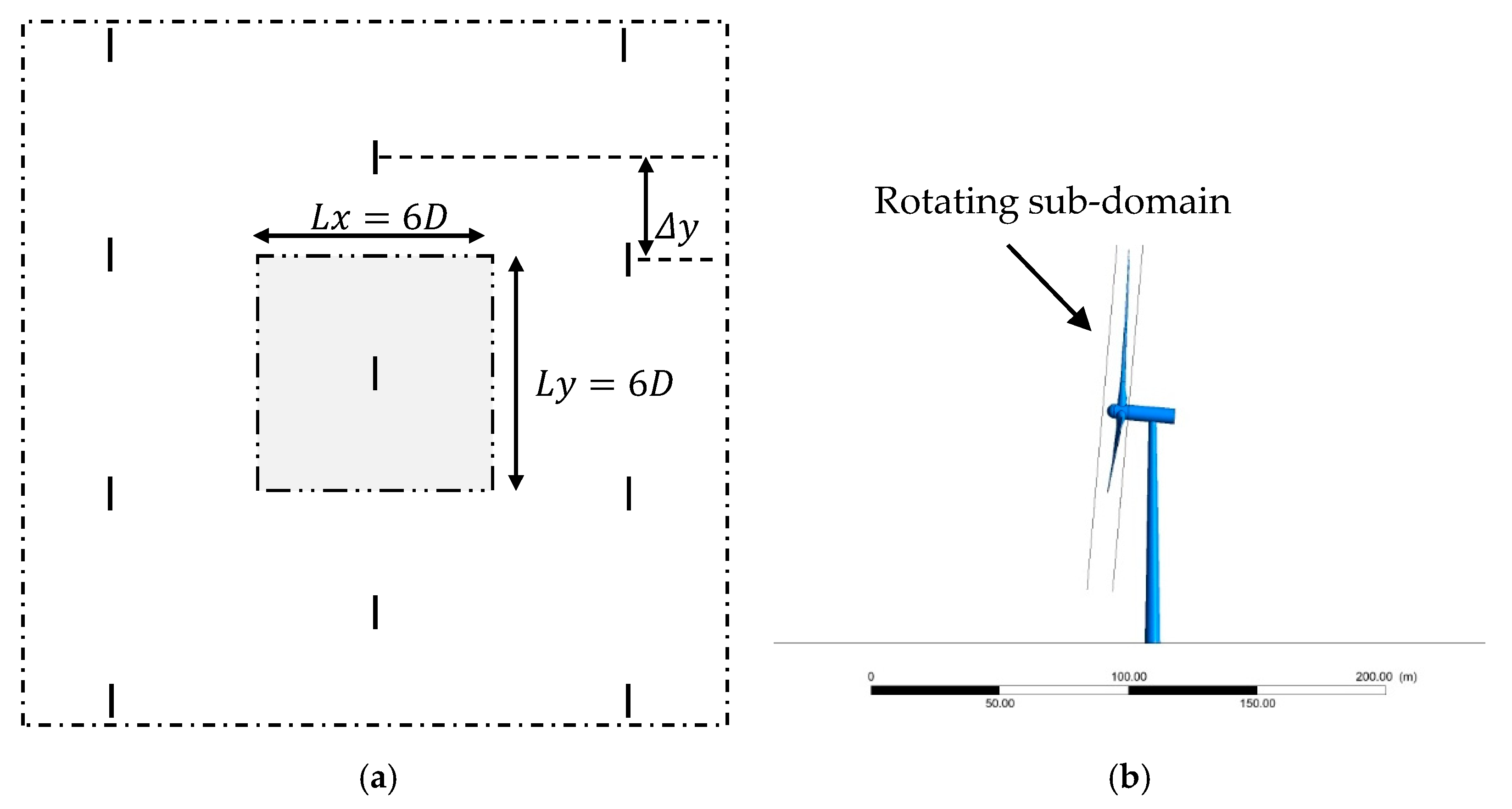
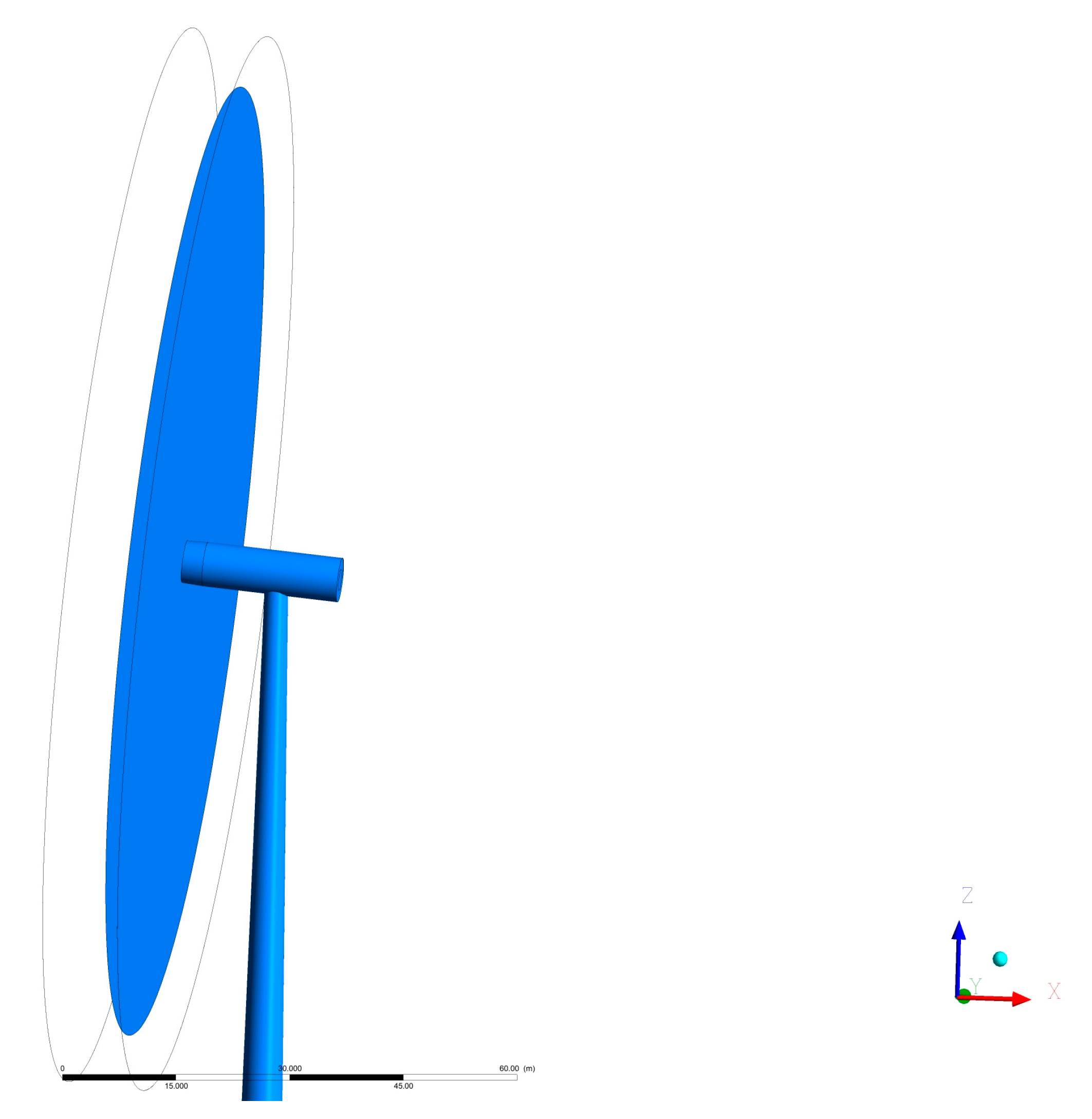
2.1. Turbine and Domain Geometries

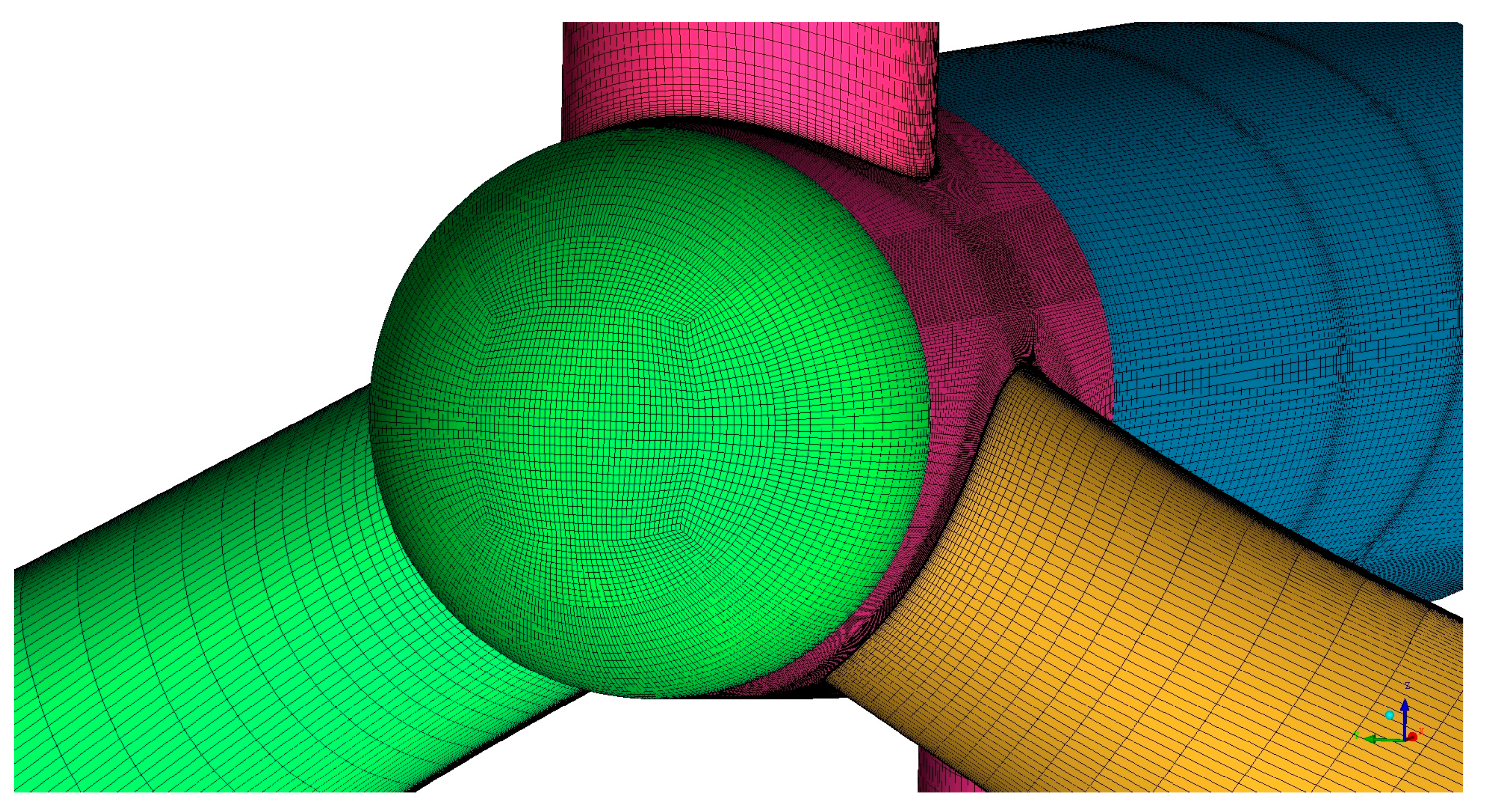
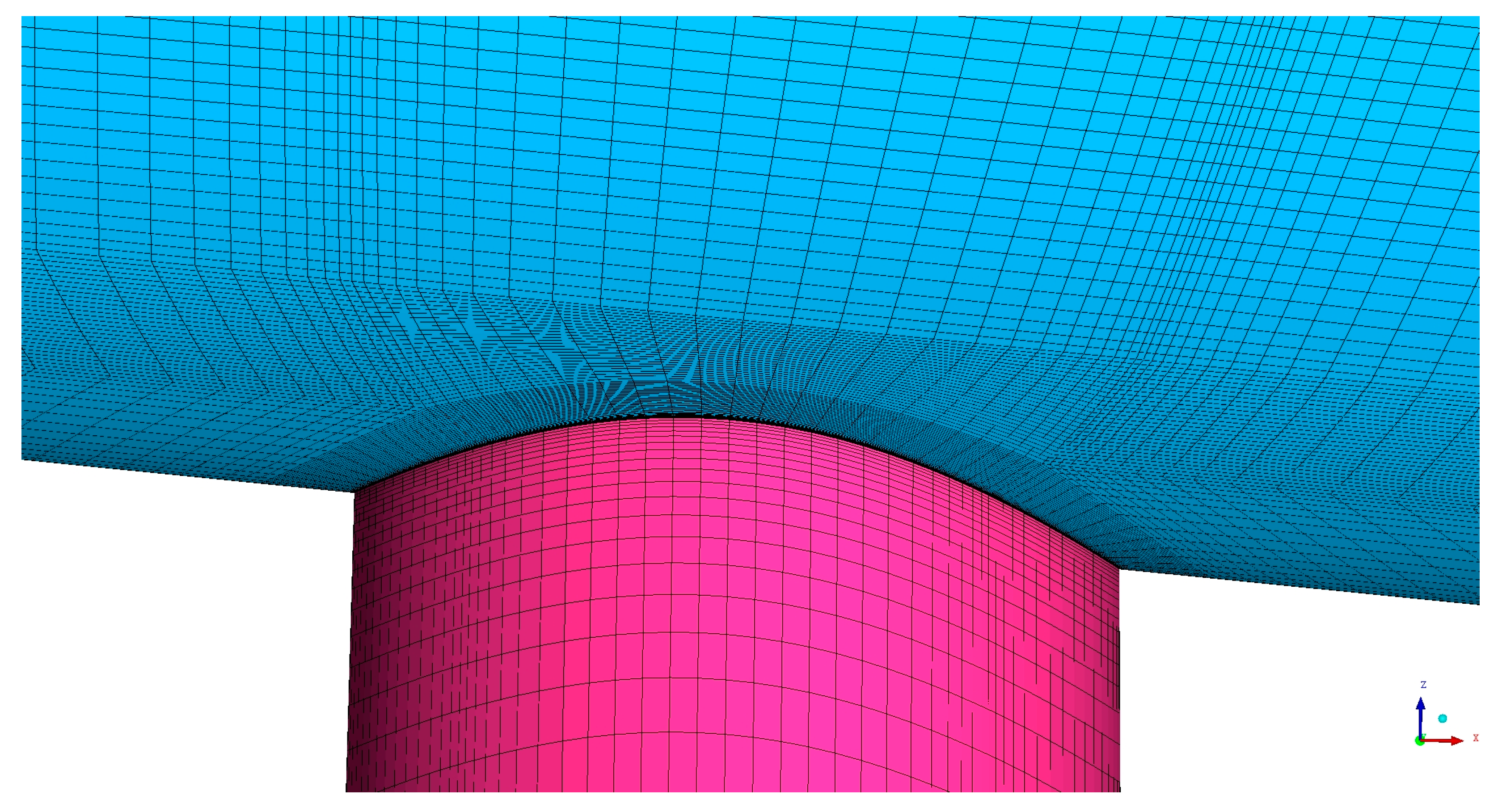
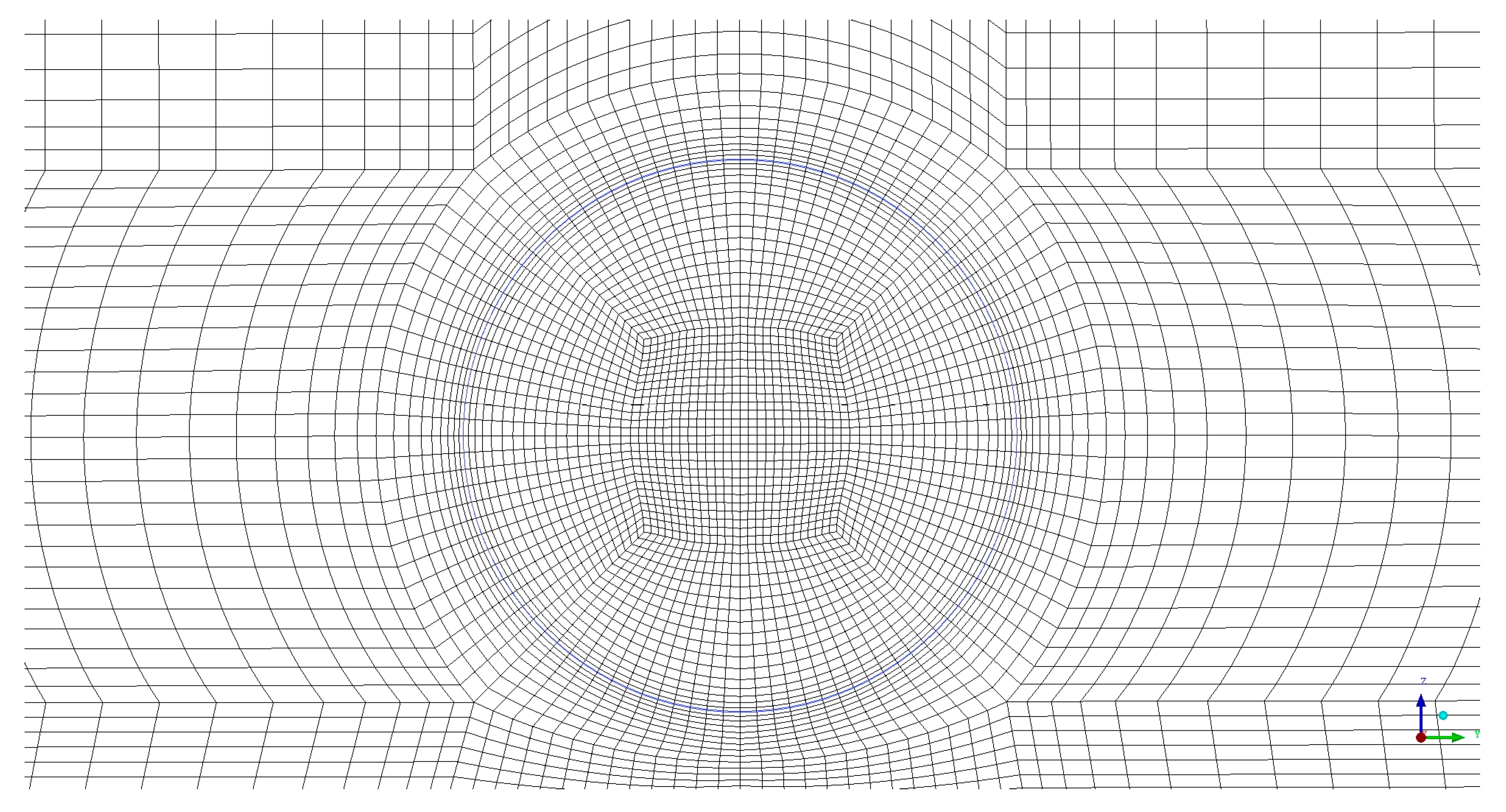
The turbine design used in this study was the NREL 5 MW three-blade model [20], which has a diameter (D) of 126 m. We also considered the alterations suggested by Sandia National Laboratories [21]: an additional smoothing process was applied to blade thickness distribution, as well as root–blade transition. Furthermore, as the tip shape was not specified in the reference designs, a ‘rounded’ tip design approach was used in this study (Figure 1), in a similar way to Bazilev et al. [24]. In addition, to simplify the construction process of a fully structured mesh, the hub diameter was increased to 5.4 m (3 m in the original design). As a consequence, a small part of the root of each blade was hidden by the enlarged hub, which was believed to not significantly affect the aerodynamics of the whole rotor. The hub centre was 90 m above the ground, equivalent to $0.21D$ ground clearance. There was 5° (respect to the horizontal plane) tilt angle applied to the rotational axis and a 2.5° precone, as defined in [20]. The original report states that the turbine tower base diameter is 6 m and the top diameter (at 87.6 m where the tower is connected to the nacelle) is 3.87 m [20]. To simplify the 3D modelling and meshing process, we used a slightly narrower design for the tower in this study. The base diameter was still 6 m, and the tower diameter at the nacelle and tower interaction was 3.14 m.

All simulations in this study considered a fully developed boundary layer flow over an infinitely large wind farm, which was modelled as a fully periodic array of turbines (Figure 2a). The outer domain size was $L_x=L_y=6D$ and $L_z=8D$, representing reasonable turbine spacing within a wind farm. The turbine rotor was placed inside a rotating cylindrical subdomain (diameter = $1.1D$ and thickness = $0.079D$ (10 m)), as shown in Figure 2b. As for the AD model, the configuration was the same as in the previous study [19], using a 126 m diameter disc whose centre was located at $x=y=0$ m and $z=90$ m, to allow a direct comparison with the FR model.

2.2. Meshing

For the purpose of this study, the boundary layers on the blades and tower were resolved (with $y_{max }^{+} ~ 1$), but wall functions were applied on the hub and nacelle surfaces in order to reduce the total number of cells. In addition, wall boundary conditions with a specific roughness height were applied on the bottom surface (representing a hypothetical ground or sea surface conditions) [19,22]. Therefore, the bottom surface was treated as a solid wall during this meshing stage.

The surface mesh of the blades was created on one blade with O-grid topology and then copied to the other two blades. There were 111 nodes in the blade spanwise direction. The spanwise cell sizes at each end of the blade were 0.001 m (next to the hub) and 0.0015 m (at the tip), and the largest size was 1.8 m (in the middle section of the blade). In the chordwise direction, 190 nodes were distributed. Although it was infeasible to conduct a mesh sensitivity study for the entire rotor, we carefully designed the blade surface mesh according to the results of existing mesh sensitivity studies in the literature. For example, a recent study showed that, for an NACA 64-618 aerofoil profile, under similar flow conditions, grid independence could be achieved when the total node number was above 180 around the aerofoil [25]. Figure 3 shows part of the complete surface mesh of the rotor. The streamwise cell sizes were 0.5 m and 0.1 m immediately upstream and downstream of the rotating subdomain, respectively. Away from the rotating subdomain, the largest streamwise spacing was 6 m and largest lateral spacing was 7 m. The first cell above the ground was 1 m high across the entire domain for the ‘without tower’ mesh. For the ‘with tower’ case, the tower was added to the existing outer domain mesh, with moderate modifications. For the node distribution on the tower surface, there were 115 nodes distributed in the circumferential direction of the tower (Figure 4), and 87 nodes were used along the tower height. Near to the tower bottom, the height of the first cell above the ground was reduced slightly, for better consistency and keeping reasonable cell aspect ratios. Overall, this mesh for the FR with tower contained $17.1\times {10}^6$ cells.

We used slightly different meshing approaches for the AD with and without tower models. The AD model had 104 nodes along the disc edge, and an ‘O-grid’ mesh topology was used inside and around the disc (Figure 5). For the AD only case, the rest of the mesh was built around the disc without creating a subdomain. The streamwise node spacing started from 0.5 m and expanded to 11 m at the inlet and outlet boundaries, and the total number of cells for the AD only model was $8\times {10}^5$. For the AD + tower case, we used the same outer domain mesh as the FR + tower case (which contained the nacelle and tower). Then, the blade-resolved rotor model was replaced by the AD model inside the rotor subdomain (Figure 6). The mesh construction was slightly modified inside the subdomain in order to accommodate the AD model. The ‘AD + tower’ mesh contained $12.2\times {10}^6$ cells. A summary of the four different meshes created is shown in

Table 1. Summary of the number of cells for each case.

	FR + Tower	FR	AD + Tower	AD
Rotor subdomain	$5.8\times {10}^6$	$5.8\times {10}^6$	$0.9\times {10}^6$	N/A
Outer domain	$11.3\times {10}^6$	$6.8\times {10}^6$	$11.3\times {10}^6$	N/A
Total	$17.1\times {10}^6$	$12.6\times {10}^6$	$12.2\times {10}^6$	$0.8\times {10}^6$

.

The FR and AD models were previously tested in an isolated (not periodic) flow condition [19], and the results were in good agreement with [20].

2.3. RANS Setup

For the majority of the CFD simulations in this study, the Reynolds-averaged Navier–Stokes (RANS) equations were solved using the commercial CFD solver ‘ANSYS FLUENT 17.2’ [26] with the k–ω SST turbulence model [27]. The density and dynamic viscosity of the working fluid (air) were $\rho =1.225 \mathrm{kg}/{\mathrm{m}}^3$ and $\mu =1.7894\times {10}^{-5} \mathrm{kg}/\left(\mathrm{ms}\right)$, respectively. The bottom boundary condition for all simulations was set as ‘wall’ [26], with a nominal roughness height $K_s=1 \mathrm{m}$ and the empirical constant $E$ and roughness constant $C_s$ values were kept as 9.793 and 0.5, respectively (this corresponds to an aerodynamic roughness length of $z_0=0.051$ m since $K_s=\left(E/C_S\right)z_0$ [28]). The top boundary was set as ‘symmetry’. Periodic conditions were applied to both streamwise and lateral ends of the domain. However, the streamwise ends (or the inlet and outlet interface) were split vertically in the middle into two parts, where the right inlet was connected to the left outlet and vice versa. This allowed us to simulate an infinitely large fully staggered turbine array, as previously shown in Figure 2a.

In order to decide the background pressure gradient inside the periodic domain, an ‘empty box’ simulation [19,22] with a fixed mass flow rate was conducted first. This simulation (steady RANS) was carried out using the ‘AD only’ mesh, with the disc boundary condition set as ‘interior’. This fixed mass flow rate was calculated using a power-law velocity profile (with an exponent of 0.1) with reference wind speed $U_{ref}=15\mathrm{m}/\mathrm{s}$ at $z=90 \mathrm{m}$ (hub level). This resulted in a farm-averaged wind speed below the rated wind speed for the NREL 5 MW turbine (11.4 m/s) in this study. The pressure gradient obtained from this empty box simulation was $-7.49\times {10}^{-4} \mathrm{Pa}/\mathrm{m}$, which was used as the driving force of the wind flow for all wind farm simulations in this study. This was based on the assumption that, for an infinitely large wind farm, the driving force of the wind is not affected by the existence of wind turbines [1,22]. In reality, the driving force of wind over a large (finite-size) wind farm should depend on the characteristics of mesoscale atmospheric response [29,30]. To obtain the correct driving force and, thus, the correct wind speed for a real wind farm, we would need to assess the ‘extractability’ of wind at a given wind farm site using a mesoscale weather model [30], but this is outside the scope of the present study.

2.3.1. AD Simulations

In the AD simulations (using steady RANS), the effect of the rotor was modelled as streamwise momentum losses, i.e., as a stationary porous surface of zero thickness with a momentum loss factor $K$ [22]. To obtain the most appropriate $K$ value, a few isolated actuator disc simulations were conducted by Delafin et al. [19] prior to the current study. Different $K$ values were tested to obtain a $C_T$ (thrust coefficient) value as close as possible to an isolated FR turbine simulation (with TSR = 7.0) in [19]. The most appropriate value was found to be K = 1.2825, yielding an area-averaged streamwise velocity over the AD, $U_{T single}=8.666 \mathrm{m}/\mathrm{s}$. The SIMPLE algorithm was used for pressure–velocity coupling, and the second-order upwind scheme was used for the discretisation of the momentum and turbulence model equations. Both AD simulations (with and without tower) were run for ${10}^6$ iterations to obtain fully converged results.

2.3.2. FR Simulations

The FR simulations were carried out using unsteady RANS. All turbine surfaces were considered as ‘wall’. The rotating motion of the rotor (with a fixed rotating speed of 7.703 rpm) was achieved by applying the ‘sliding mesh’ method to the subdomain containing the turbine rotor. Since the velocity profile inside the fully developed farm boundary layer was not known a priori, the rotating speed was determined using AD simulation results, to match the tip speed ratio (TSR) with the ‘optimal’ value (TSR = 7.0) reported in [20]. Specifically, we assumed a proportional relationship between the rotor rpm and $U_T$ values (obtained from AD simulations for the single turbine case and for the periodic farm case, respectively) to determine the rotational speed for the FR farm simulations.

$$\frac{RP{M}_{single}}{RP{M}_{farm}}=\frac{U_{T single}}{U_{T farm}} \to \frac{12.1 \mathrm{rpm}}{RP{M}_{farm}}=\frac{8.666\mathrm{m}/\mathrm{s}}{5.517\mathrm{m}/\mathrm{s}} \to RP{M}_{farm}=7.703 \mathrm{rpm}$$

(1)

where $U_{T farm}$ was obtained from the ‘AD only’ (without tower) farm simulation. Once the rotational speed was determined, the timestep size was set as $\mathsf{\Delta }t=0.0108 \mathrm{s}$ (which led to a rotor azimuthal angle of $\mathsf{\Delta }\theta =0.5°$ per timestep), and 15 iterations were conducted per timestep. It should be noted that this rotational speed was for the ‘FR rotor only’ (without tower) simulation. As shown later, adding the tower to the model reduced the average wind speed across the domain. This means that the rotational speed would need to be slightly altered after adding the tower, in order to achieve the same TSR as the rotor only case. However, in this study, we used the same rotational speed (7.703 rpm) for both ‘tower’ and ‘no tower’ cases for simplicity. After completing the FR simulations, the difference in TSR between the ‘tower’ and ‘no tower’ cases was approximately 2.1%, which can be considered negligible. According to a recent study [31], a small TSR variation would not cause noticeable changes in turbine performance (approximately 0.53% difference in power output).

To quickly generate a fully developed atmospheric boundary layer flow for the FR simulations, the flow field obtained from the AD simulations was applied as the initial flow conditions. The ‘Coupled’ algorithm [26] was employed for pressure–velocity coupling. A second-order implicit scheme was used for the temporal discretisation, and the second-order upwind scheme was used for spatial discretisation of the momentum and turbulence model equations. The FR simulations (with and without tower) were run for 100 revolutions first, and then additional 18 revolutions were carried out to calculate time-averaged results to be compared with the theoretical model [22]. For the FR with tower case, it took about 13 h to run one revolution simulation on 128 CPUs.

2.4. DDES Setup

In addition to the URANS simulations, we also attempted to run DDES for the FR with tower case. The k–ω SST turbulence model was switched from its URANS mode to DDES mode available in FLUENT [26] after the first 100 revolutions of URANS simulations. All boundary conditions were unchanged. We also used the same fixed RPM as we used in URANS, although this meant that the TSR fluctuated more in DDES (about 20.2%) than in URANS (about 3.5%). A bounded central differencing scheme was used for the spatial discretisation of the momentum equations, and a bounded second-order implicit scheme was employed for the temporal discretisation. The DDES was run only for 54 revolutions due to the limited availability of computational resources.

2.5. Postprocessing of URANS Results

The rotor moment coefficient, $C_m$, is defined as

$$C_m=\frac{\tau }{\frac{1}{2}\rho Ar{U}_{F0}^2}$$

(2)

where $\tau$ is the torque of the rotor, $A$ is the swept area of the rotor ($A=\pi r^2$), $r$ is the radius of the rotor, and $U_{F0}$ is the natural farm-layer wind speed obtained from the ‘empty box’ simulation. The power output of the rotor is calculated as,

$$P=\tau · \omega$$

(3)

where $\omega$ is the rotational speed of the turbine (0.8067 rad/s for the farm simulations and 1.267 rad/s for the isolated turbine simulation).

3. Results and Discussion

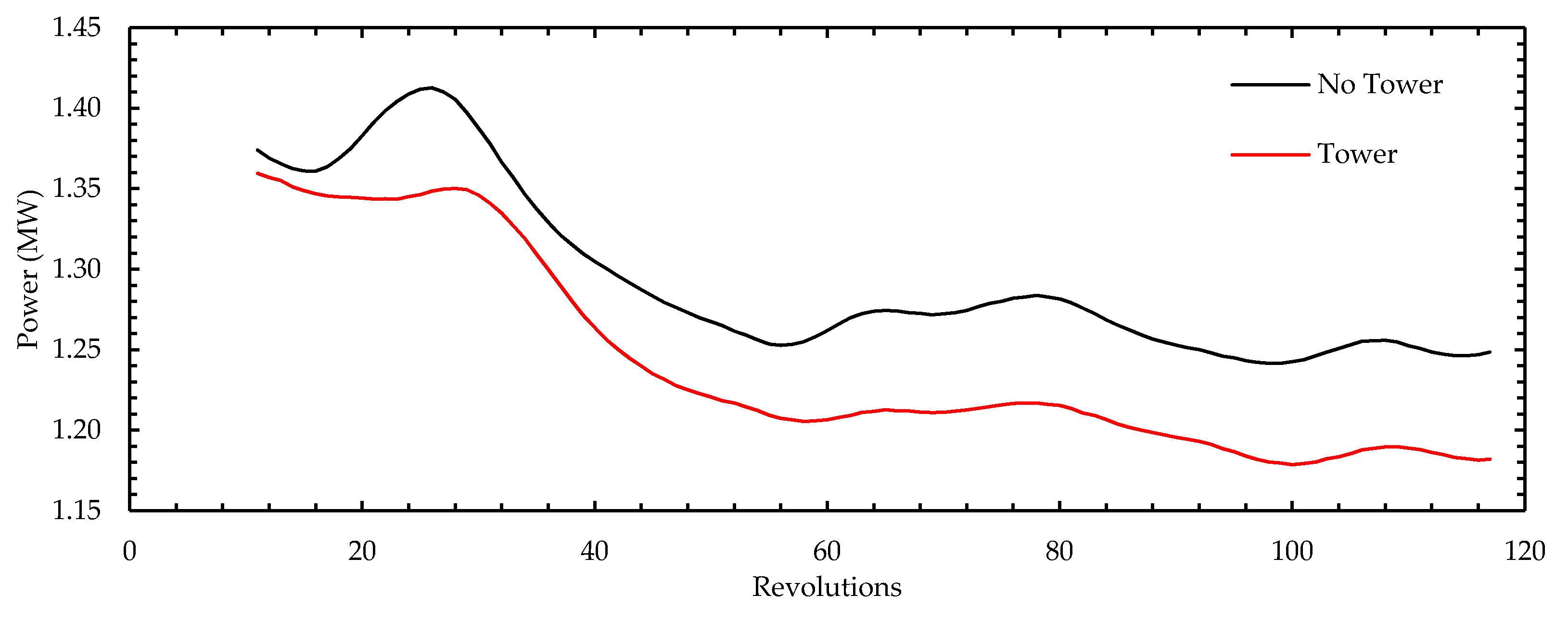
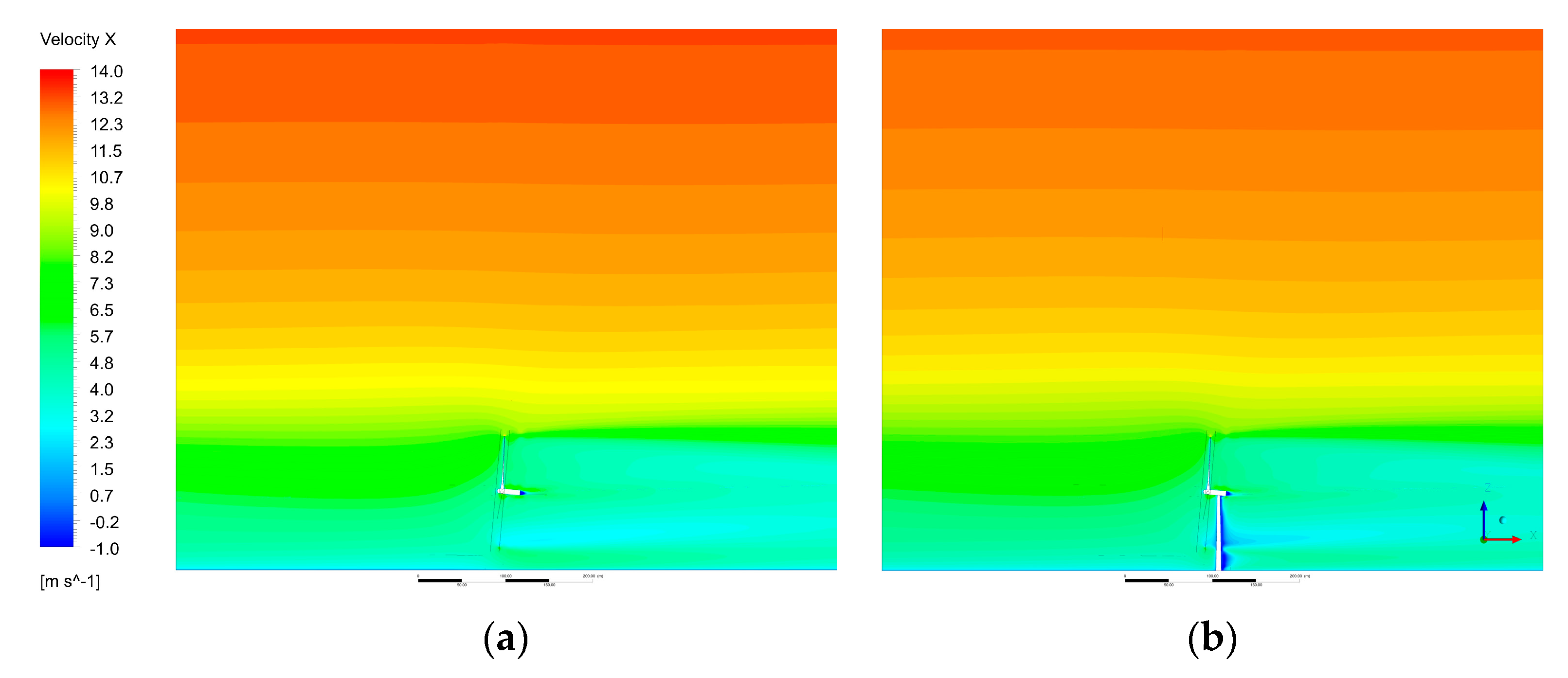
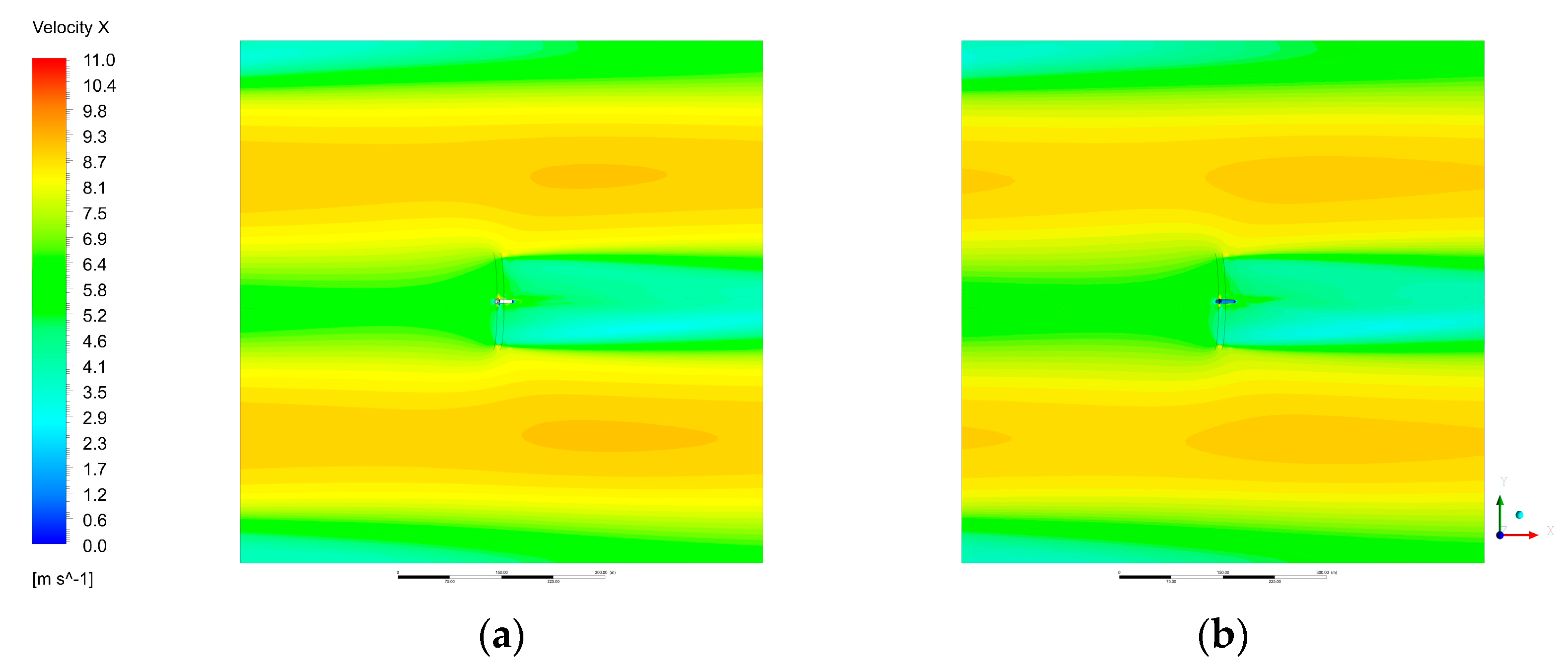
3.1. URANS

Figure 7 shows the time histories of the turbine power output observed in the FR-URANS simulations with and without the tower. It can be seen that, for both cases, a large number of rotor revolutions were required for the power to reach a quasi-stationary state. A consistent difference of about 0.06 MW (5%) between the two cases was observed after around 100 revolutions. This clearly shows that the predicted power was reduced by adding the turbine tower to the model.

The flow field comparison between ‘tower’ and ‘no tower’ cases is shown in Figure 8 and Figure 9; the former is plotted on a vertical plane that goes through the centre of the turbine, and the latter is plotted on the horizontal plane at the hub centre level (90 m above the ground). The tower generated its own wake and, thus, enlarged the velocity deficit behind the lower part of the rotor. This can also be observed in the velocity profiles plotted in Figure 10, especially at $x/D=0.5$, where there was a noticeable speed reduction close to the ground due to the turbine tower. However, a more important effect of the tower in this study is that it reduced the wind speed above the turbine (Figure 8). This is because the additional flow resistance (or drag) created by the tower contributed to a stronger development of the internal boundary layer (IBL). In other words, the slower wind speed observed above a given turbine was not because of the tower of that turbine, but because of the towers of other turbines located upstream (note that there are an infinite number of turbines located upstream of the turbine shown in Figure 8, due to the periodicity). It is clear from Figure 10 that this reduction in wind speed above the turbine was observed at any streamwise positions, confirming that this is a farm-scale (rather than a local/turbine-scale) wind speed reduction. On the other hand, the wind speed difference observed behind the tower diminished quickly towards downstream due to strong turbine-scale wake mixing, and the flow profiles further downstream appeared almost identical between ‘no tower’ and ‘tower’ cases (Figure 10d).

The AD (with and without tower) RANS results are also plotted in Figure 10 for comparison. Between the AD and FR cases, the differences in flow profiles were mostly within the rotor region (approximately $0.21<z/D<1.21$). In addition, the AD results also showed that the tower reduced the wind velocity at higher positions. It is remarkable that the wind profiles above the top of the turbine ($z/D>1.21$) were almost identical between the AD with/without tower and the FR with/without tower cases. This highlights a key finding that the choice of the rotor model (AD or FR) does not affect the prediction of the tower effect on the farm-scale wind speed reduction. This finding supports the argument that the AD model (with tower) would be sufficient to predict the wind farm blockage effect. This is discussed further in Section 3.3.

3.2. DDES

As shown in Figure 11a, the turbine power output started to deviate from the URANS results about 13 revolutions after switching to DDES, and then large fluctuations started to occur. Since the average wind speed at the hub height was about 8 m/s, these 13 revolutions approximately correspond to the time required for the hub height wind to travel through the periodic domain once. Although not shown here for brevity, the turbine thrust also fluctuated in a very similar manner to the power output. Such fluctuations of the blade loadings were also reported in a previous LES study of a single rotating blade of the NREL 5 MW turbine interacting with realistic atmospheric turbulence [32]. The time history (recorded every four timesteps) of the streamwise velocity measured at $2.5D$ upstream of the turbine (at the hub height) is plotted in Figure 11b. By comparing the two figures, it can be seen that the power output fluctuations were closely correlated with the upstream velocity fluctuations.

Figure 12 shows an example of instantaneous velocity contours on vertical and horizontal planes, visualising the turbulent flow field around the turbine. The flow in the top half of the domain did not contain any turbulent eddies; this is presumably because the simulation was not run long enough, but this may also be because of the relatively small horizontal size of the domain used in this study. Nevertheless, the flow at the turbine level appeared to be already fully turbulent (Figure 13 and Figure 14).

Figure 15 and Figure 16 show the instantaneous vortical flow structures obtained from URANS and DDES results. These vortex structures were visualised using iso-surfaces of the Q-Criterion, and the colour scheme is based on the instantaneous streamwise velocity. Seven identical flow fields obtained from the original single-turbine domain are plotted together in these figures, in order to better visualise the flow structures over the staggered array of turbines (see Figure 2). As expected, the URANS results (Figure 15) show only some strong turbine-generated vortices, such as tip and hub vortices. On the other hand, the DDES results (Figure 16, using the same Q-Criterion values as in Figure 15) show much more complex turbulent flow structures created in the wake region and how they interacted with the strong turbine-generated vortices. It is remarkable that some large hairpin-like vortices were also visible in front of the turbine, similarly to those commonly appearing near the top of a turbulent boundary layer [33].

3.3. Comparison with Theoretical Model

In this section, we compare the AD-RANS and FR-URANS simulation results with the theoretical model of an infinitely large wind farm reported earlier in [22]. For the calculation of the tower resistance in the theoretical model, we employed a typical drag coefficient of a circular cylinder (at a corresponding Reynolds number) of 0.6. A summary of the comparison is shown in

Table 2. Comparison of AD-RANS, FR-URANS, and theoretical model predictions.

		${\mathit{C}}_{\mathit{P}}$	${\mathit{C}}_{\mathit{P}}^{*}$	${\mathit{C}}_{\mathit{T}}$	${\mathit{C}}_{\mathit{T}}^{*}$
AD-RANS	No Tower	0.0651	0.414	0.176	0.603
	Tower	0.0641	0.412	0.174	0.601
	Diff.%	1.55%	0.52%	1.04%	0.35%
FR-URANS	No Tower	0.0495	0.303	0.167	0.561
	Tower	0.0469	0.306	0.163	0.570
	Diff.%	5.21%	−0.90%	2.48%	−1.67%
Theoretical model [22]	No Tower	0.0622	0.380	0.198	0.570
	Tower	0.0607	0.380	0.195	0.570
	Diff.%	2.50%	0.00%	1.68%	0.00%

. The wind farm power and thrust coefficients ($C_P$ and $C_T$) were calculated as $C_P=P/\frac{1}{2}\rho A{U}_{F0}^3$ and $C_T=T/\frac{1}{2}\rho A{U}_{F0}^2$, respectively, whereas the ‘local’ power and thrust coefficients ($C_P^{*}$ and $C_T^{*}$) were calculated using $U_F$ (farm-layer-average wind speed, see [22] for details) instead of $U_{F0}$. Note that the $C_P$ and $C_T$ values were very small in this study as we considered an infinitely large wind farm with a fixed driving force of the wind. The $C_P$ values calculated from the AD-RANS simulations were very close to the theoretical model predictions, and the $C_T$ values were also closer to the theoretical results compared to the FR-URANS results. This agrees with the findings in the previous study (for the same NREL 5 MW rotor without a tower) [19].

As for the effect of the tower, both AD-RANS and FR-URANS simulations agreed fairly well with the theoretical model predictions as summarised in Table 2. The $C_P$ and $C_T$ values were slightly (about 1 to 5%) lower due to the additional farm-scale wind speed reduction caused by the tower, whereas its effects on the $C_P^{*}$ and $C_T^{*}$ values seemed negligibly small. The effect of the tower on $C_P$ was a little underestimated by the AD-RANS (1.55%) and the theoretical model (2.50%) compared to the FR-URANS (5.21%), showing the limitation of the methods based on the classical actuator disc theory. A possible solution to this problem would be to replace the actuator disc part of the theoretical model with the blade element momentum (BEM) theory. This modification (called the ‘BEM-farm-momentum’ method) has already been reported in [34] but only for the case without the tower. Therefore, it would be useful to also apply this method to the case with the tower in a future study.

4. Conclusions

In this paper, we presented blade-resolved CFD simulations of the NREL 5 MW wind turbine placed in a horizontally periodic domain, representing an infinitely large wind farm. Three main wind farm simulations were conducted in this study, namely, FR-URANS ‘without tower’, FR-URANS ‘with tower’, and FR-DDES ‘with tower’. Two additional wind farm simulations using steady RANS with a simple AD model were also conducted for comparison. The FR-URANS results showed substantial effects of the tower on the overall wind farm efficiency, with a decrease of about 5% in the total power due to the additional tower drag (under the assumption that the driving force of wind over the wind farm was unchanged). This further confirms the importance of including turbine support structures in the modelling of large wind farms, which agrees with the findings reported earlier in [22,35].

We also showed that the AD-RANS and FR-URANS simulations predicted nearly identical velocity profiles above the wind farm (for each of the cases with and without the tower). This suggests that the simple AD model can capture the farm-scale wind speed reduction as accurately as the FR model does. In addition, both AD and FR simulations agreed fairly well with the theoretical model reported earlier in [22] in terms of the tower effect on the overall thrust (or drag) of the wind farm. However, the FR-URANS results showed a larger power reduction due to the tower (5.21%) compared to the AD-RANS (1.55%) and the theoretical model (2.50%).

The discrepancy between the FR-URANS and the theoretical model seemed largely due to the limitation of the actuator disc theory employed in the theoretical model. It may, therefore, be beneficial to replace the actuator disc part of the current theoretical model with BEM (as proposed for the case without the tower in [34]) in future studies. The FR-URANS results could be used to validate and/or improve such an extended theoretical wind farm model in future studies.

The FR-DDES results presented in this paper also provide useful information on 3D vortical flow structures over a periodic array of wind turbines, e.g., the interaction of large hairpin-like vortices with small but strong blade-tip vortices. However, due to limited computational resources, it was not possible in this study to obtain meaningful time-averaged results from the DDES for the wind farm performance. We found that the computational cost of the FR-DDES required for a given number of turbine revolutions is very similar to the corresponding FR-URANS simulation, but the sampling period required is much longer as the timescale for the fluctuation of the flow field is much longer than that for the turbine revolution.

References

1. Nishino, T. Two-scale momentum theory for very large wind farms. J. Phys. Conf. Ser. 2016, 753, 32054. [Google Scholar] [CrossRef]
2. Wu, Y.T.; Porté-Agel, F. Large-Eddy Simulation of Wind-Turbine Wakes: Evaluation of Turbine Parametrisations. Bound.-Layer Meteorol. 2011, 138, 345–366. [Google Scholar] [CrossRef]
3. Naderi, S.; Parvanehmasiha, S.; Torabi, F. Modeling of horizontal axis wind turbine wakes in Horns Rev offshore wind farm using an improved actuator disc model coupled with computational fluid dynamic. Energy Convers. Manag. 2018, 171, 953–968. [Google Scholar] [CrossRef]
4. Richmond, M.; Antoniadis, A.; Wang, L.; Kolios, A.; Al-Sanad, S.; Parol, J. Evaluation of an offshore wind farm computational fluid dynamics model against operational site data. Ocean Eng. 2019, 193, 106579. [Google Scholar] [CrossRef]
5. Stevens, R.J.; Martínez-Tossas, L.A.; Meneveau, C. Comparison of wind farm large eddy simulations using actuator disk and actuator line models with wind tunnel experiments. Renew. Energy 2017, 116, 470–478. [Google Scholar] [CrossRef]
6. Sørensen, J.N.; Mikkelsen, R.F.; Henningson, D.S.; Ivanell, S.; Sarmast, S.; Andersen, S.J. Simulation of wind turbine wakes using the actuator line technique. Phil. Trans. R. Soc. 2015, 373, 20140071. [Google Scholar] [CrossRef] [Green Version]
7. Kalvig, S.; Manger, E.; Hjertager, B. Comparing different CFD wind turbine modelling approaches with wind tunnel measurements. J. Phys. Conf. Ser. 2014, 555, 012056. [Google Scholar] [CrossRef] [Green Version]
8. Madsen, M.H.A.; Zahle, F.; Sørensen, N.N.; Martins, J.R.R.A. Multipoint high-fidelity CFD- based aerodynamic shape optimization of a 10 MW wind turbine. Wind Energ. Sci. 2019, 4, 163–192. [Google Scholar] [CrossRef] [Green Version]
9. Rodrigues, R.V.; Lengsfeld, C. Development of a Computational System to Improve Wind Farm Layout, Part I: Model Validation and Near Wake Analysis. Energies 2019, 12, 940. [Google Scholar] [CrossRef] [Green Version]
10. Stergiannis, N.; Lacor, C.; Beeck, J.V.; Donnelly, R. CFD modelling approaches against single wind turbine wake measurements using RANS. J. Phys. Conf. Ser. 2016, 753, 032062. [Google Scholar] [CrossRef]
11. Uchida, T.; Taniyama, Y.; Fukatani, Y.; Nakano, M.; Bai, Z.; Yoshida, T.; Inui, M. A New Wind Turbine CFD Modeling Method Based on a Porous Disk Approach for Practical Wind Farm Design. Energies 2020, 13, 3197. [Google Scholar] [CrossRef]
12. Weihing, P.; Schulz, C.; Lutz, T.; Krämer, E. Comparison of the Actuator Line Model with Fully Resolved Simulations in Complex Environmental Conditions. J. Phys. Conf. Ser. 2017, 854, 012049. [Google Scholar] [CrossRef]
13. Miao, W.; Li, C.; Pavesi, G.; Yang, J.; Xie, X. Investigation of wake characteristics of a yawed HAWT and its impactson the inline downstream wind turbine using unsteady CFD. J. Wind. Eng. Ind. Aerodyn. 2017, 168, 60–71. [Google Scholar] [CrossRef]
14. Wilson, J.M.; Davis, C.J.; Venayagamoorthy, S.K.; Heyliger, P.R. Comparisons of Horizontal-Axis Wind Turbine Wake Interaction Models. J. Sol. Energ. Eng. 2015, 137, 031001. [Google Scholar] [CrossRef]
15. Zahle, F.; Sørensen, N.N.; Johansen, J. Wind Turbine Rotor-Tower Interaction Using an Incompressible Overset Grid Method. Wind Energy 2009, 12, 594–619. [Google Scholar] [CrossRef]
16. Hand, M.M.; Simms, D.A.; Fingersh, L.J.; Jager, D.W.; Cotrell, J.R.; Schreck, S.; Larwood, S.M. Unsteady Aerodynamics Experiment Phase VI: Wind Tunnel Test Configurations and Available Data Campaigns. Tech. Rep. 2001, 15000240. [Google Scholar] [CrossRef] [Green Version]
17. Rodrigues, R.V.; Lengsfeld, C. Development of a Computational System to Improve Wind Farm Layout, Part II: Wind Turbine Wakes Interaction. Energies 2019, 12, 1328. [Google Scholar] [CrossRef] [Green Version]
18. Schepers, J.G.; Boorsma, K.; Cho, T.; Gomez-Iradi, S.; Schaffarczyk, P.; Jeromin, A.; Shen, W.Z.; Lutz, T.; Meister, K.; Stoevesandt, B. Final Report of IEA Task 29, Mexnet (Phase 1): Analysis of Mexico Wind Tunnel Measurements; Technical University of Denmark: Lyngby, Denmark, 2012. [Google Scholar]
19. Delafin, P.-L.; Nishino, T. Momentum balance in a fully developed boundary layer over a staggered array of NREL 5MW rotors. J. Phys. Conf. Ser. 2017, 854, 12009. [Google Scholar] [CrossRef] [Green Version]
20. Jonkman, J.; Butterfield, S.; Musial, W.; Scoot, G. Definition of a 5-MW Reference Wind Turbine for Offshore System Development. Tech. Rep. 2009, 947422. [Google Scholar] [CrossRef] [Green Version]
21. Resor, B.R. Definition of a 5MW/61.5m wind turbine blade reference model. Tech. Rep. 2013, 1095962. [Google Scholar] [CrossRef] [Green Version]
22. Ma, L.; Nishino, T.; Antoniadis, A. Prediction of the impact of support structures on the aerodynamic performance of large wind farms. J. Renew. Sustain. Energy 2019, 11, 063306. [Google Scholar] [CrossRef]
23. Nishino, T.; Dunstan, T.D. Two-scale momentum theory for time-dependent modelling of large wind farms. J. Fluid Mech. 2020, 894, A2. [Google Scholar] [CrossRef]
24. Bazilevs, Y.; Hsu, M.-C.; Akkerman, I.; Wright, S.; Takizawa, K.; Henicke, B.; Spielman, T.; Tezduyar, T.E. 3D simulation of wind turbine rotors at full scale. Part I: Geometry modeling and aerodynamics. Int. J. Numer. Meth. Fluids 2011, 65, 207–235. [Google Scholar] [CrossRef] [Green Version]
25. Major, D.; Palacios, J.; Maufhumer, M.; Schmitz, S. A Numerical Model for the Analysis of Leading-Edge Protection Tapes for Wind Turbine Blades. J. Phys. Conf. Ser. 2020, 1452, 12058. [Google Scholar] [CrossRef] [Green Version]
26. ANSYS Inc. ANSYS Fluent User’s Guide Release 17.2; ANSYS Inc.: Canonsburg, PA, USA, 2016. [Google Scholar]
27. Menter, F.R. Two-Equation Eddy-Viscosity Turbulence Models for Engineering Applications. AIAA J. 1994, 32, 1598–1605. [Google Scholar] [CrossRef] [Green Version]
28. Blocken, B.; Stathopoulos, T.; Carmeliet, J. CFD simulation of the atmospheric boundary layer: Wall function problems. Atmos. Environ. 2007, 41, 238–252. [Google Scholar] [CrossRef]
29. Bleeg, J.; Purcell, M.; Ruisi, R.; Traiger, E. Wind farm blockage and the consequences of neglecting its impact on energy production. Energies 2018, 11, 1609. [Google Scholar] [CrossRef] [Green Version]
30. Patel, K.; Dunstan, T.D.; Nishino, T. Time-dependent upper limits to the performance of large wind farms due to mesoscale atmospheric response. Energies 2021, 14, 6437. [Google Scholar] [CrossRef]
31. Pinto, M.L.; Franzini, G.R.; Simos, A.S. A CFD analysis of NREL’s 5MW wind turbine in full and model scales. J. Ocean Eng. Mar. Energy 2020, 6, 211–220. [Google Scholar] [CrossRef]
32. Vijayakumar, G.; Brasseur, J.G.; Lavely, A.; Jayaraman, B. Interaction of Atmospheric Turbulence with Blade Boundary Layer Dynamics on a 5MW Wind Turbine using Blade-boundary-layer-resolved CFD with hybrid URANS-LES. In Proceedings of the 34th Wind Energy Symposium, AIAA SciTech Forum, San Diego, CA, USA, 4–8 January 2016. [Google Scholar] [CrossRef]
33. Eitel-Amor, G.; Flores, O.; Schlatter, P. Hairpin vortices in turbulent boundary layers. Phys. Fluids 2015, 27, 025108. [Google Scholar] [CrossRef]
34. Nishino, T.; Hunter, W. Tuning turbine rotor design for very large wind farms. Proc. R. Soc. A 2018, 474, 237. [Google Scholar] [CrossRef] [Green Version]
35. Ma, L.; Nishino, T. Preliminary estimate of the impact of support structures on the aerodynamic performance of very large wind farms. J. Phys. Conf. Ser. 2018, 1037, 72036. [Google Scholar] [CrossRef]
Figure 1. Rounded tip shape of the blade.
Wind 02 00004 g001
Figure 2. (a) Staggered turbine array; (b) turbine geometry and rotating subdomain.
Wind 02 00004 g002
Figure 3. Surface mesh of the turbine.
Wind 02 00004 g003
Figure 4. Nacelle and tower intersection mesh details.
Wind 02 00004 g004
Figure 5. Cross-sectional view around the disc (for AD only case).
Wind 02 00004 g005
Figure 6. AD placement inside the subdomain.
Wind 02 00004 g006
Figure 7. Convergence history of revolution-averaged power output (FR-URANS model with and without tower).
Wind 02 00004 g007
Figure 8. Contours of instantaneous streamwise velocity (m/s) at the vertical centre plane (taken at 100th revolution from FR-URANS): (a) no tower; (b) with tower.
Wind 02 00004 g008
Figure 9. Contours of instantaneous streamwise velocity (m/s) at the rotor hub height (taken at 100th revolution from FR-URANS): (a) no tower; (b) with tower.
Wind 02 00004 g009
Figure 10. Streamwise velocity profiles at different locations behind the turbine: (a) x / D = 0.5 , (b) x / D = 1.5 , (c) x / D = 2.5 , (d) x / D = 5 . The dotted horizontal line indicates the top position of the turbine.
Wind 02 00004 g010
Figure 11. (a) Time history of instantaneous and revolution-averaged power outputs; (b) time history of streamwise velocity measured at hub height ( z = 90   m ) and 2.5 D upstream of the turbine ( x = 315   m ).
Wind 02 00004 g011
Figure 12. Instantaneous streamwise velocity contours (m/s) on the streamwise vertical plane across the centre of a turbine and the horizontal plane at the turbine hub-height (taken at the 154th revolution).
Wind 02 00004 g012
Figure 13. Contours of instantaneous streamwise velocity (m/s) at vertical centre plane (taken at the 154th revolution).
Wind 02 00004 g013
Figure 14. Contours of instantaneous streamwise velocity (m/s) at rotor hub height (taken at the 154th revolution).
Wind 02 00004 g014
Figure 15. Vortical flow structures over a staggered array of turbines, obtained from the FR-URANS simulation with tower (visualised using iso-surfaces of Q-Criterion).
Wind 02 00004 g015
Figure 16. Vortical flow structures over a staggered array of turbines, obtained from FR-DDES with tower (visualised using iso-surfaces of Q-Criterion, taken at the 154th revolution).
Wind 02 00004 g016