Article

An Intelligent Method for Fault Location Estimation in HVDC Cable Systems Connected to Offshore Wind Farms

by
Seyed Hassan Ashrafi Niaki
1,*,
Jalal Sahebkar Farkhani
1,
Zhe Chen
1,
Birgitte Bak-Jensen
1 and
Shuju Hu
2
1
Department of Energy Technology, Aalborg University, 9220 Aalborg, Denmark
2
Institute of Electrical Engineering, Chinese Academy of Sciences, Beijing 100049, China
*
Author to whom correspondence should be addressed.
Wind 2023, 3(3), 361-374; https://doi.org/10.3390/wind3030021
Submission received: 20 July 2023 / Revised: 5 August 2023 / Accepted: 28 August 2023 / Published: 31 August 2023
(This article belongs to the Special Issue Challenges and Perspectives of Wind Energy Technology)

Abstract

:
Large and remote offshore wind farms (OWFs) usually use voltage source converter (VSC) systems to transmit electrical power to the main network. Submarine high-voltage direct current (HVDC) cables are commonly used as transmission links. As they are liable to insulation breakdown, fault location in the HVDC cables is a major issue in these systems. Exact fault location can significantly reduce the high cost of submarine HVDC cable repair in multi-terminal networks. In this paper, a novel method is presented to find the exact location of the DC faults. The fault location is calculated using extraction of new features from voltage signals of cables’ sheaths and a trained artificial neural network (ANN). The results obtained from a simulation of a three-terminal HVDC system in power systems computer-aided design (PSCAD) environment show that the maximum percentage error of the proposed method is less than 1%.

1. Introduction

Offshore wind farms are going to become a major source of energy in the wind energy field. The energy that can be derived from offshore is more than that onshore due to the high potential of wind on the sea. There are two types of power transmission for OWFs—AC and DC [1]. Studies show that HVDC connections are more economical for large and remote OWFs [2,3]. New-generation power electronic converters are VSCs, which have demonstrated themselves to be an attractive alternative to previous generations of current source converters (CSCs) or line-commutated converters (LCCs). The VSC controls activate and reactivate power independently. They can also have appropriate interaction with main grids, especially weak grids, and various converters in the same network zone. Moreover, the VSCs occupy less space than LCCs [4,5].
In multi-terminal VSC-HVDC transmission systems, cross-linked polyethylene (XLPE) submarine cables have a significant role as DC power links. The DC submarine cable is liable to ground faults because of possible insulation breakdown. The great advancements in circuit breaker technology make multi-terminal HVDC system more feasible than in the past [6,7]. A VSC-based HVDC system has good prospects for the multi-terminal DC grid, owing to the advantages of this type of HVDC system [8]. However, there are many challenges moving from point-to-point DC topology to multi-terminal DC topology, especially in the protection system. The goal of a protection system is to maintain the power system stability by isolating only the faulty components whilst leaving as much of the network as possible still in operation [9]. In point-to-point HVDC systems, the popular solution is to employ AC circuit breakers in which the whole HVDC grid is disconnected from the rest of the network. Thus, the whole HVDC grid is de-energized in the event of a fault by the circuit breakers residing on the AC sides [10]. In the multi-terminal cases, it is preferable to isolate only the faulted section instead of the whole HVDC grid. To achieve this goal, DC circuit breakers are used to isolate only the faulted section. The DC protection relays also determine when the breakers should operate. DC protection relaying requires special consideration over conventional AC methods. Fault location for this kind of system is a great challenge due to the high cost of maintenance of faulted cables undersea. Therefore, an accurate fault location method is vital in this field.
In [11,12], a protection scheme of a multi-terminal VSC system and fault analysis for a multi-terminal DC wind farm are discussed, respectively. However, they have not investigated any fault location estimation method. In [13], DC faults are isolated in multi-terminal DC (MTDC) by using voltage and current characteristics. In this way, only the faulted DC link is isolated, and the fault location identification is neglected. A new algorithm based on a combination of traveling waves and a cross-correlation method has been proposed for the calculation of the fault location in the DC cable of both VSC and CSC HVDC systems [14]. Reference [15] utilizes noise pattern analysis caused by the switching of power electronic devices to locate ground faults in ungrounded DC shipboard power distribution systems. Active impedance estimation has been suggested for fault location in a zonal DC marine power system [16]. A fault location algorithm based on wavelet transform is investigated for VSC-HVDC cable in [17]. An iterative method based on voltage comparison is presented in [18] for the estimation of fault location in HVDC systems. Reference [19] investigates a method based on fundamental wave propagation theory to detect and discriminate faults in HVDC grids. The VSC-HVSC systems have different fault transients from those in the HVAC systems. Therefore, more studies need to be carried on protection of VSC-HVDC systems. In [20], the operation of distance relays was investigated for an offshore wind farm connected to the main grid via a VSC-HVDC system. A method based on a combination of DC and harmonic overcurrent protection for rectifier converters of monopolar HVDC systems is also presented [21]. To achieve fast protection of HVDC grids against DC faults, an algorithm in ref [22] uses sensors integrated into the cable joints and proactive hybrid breakers. Double-circuit transmission lines, with bipolar transmission lines of two different LCC-based HVDC systems constructed on the same towers, are a new technology. An integrated protection method based on traveling wave theory is presented for double-circuit HVDC links [23].
Recently, traveling wave principle-based protection was applied in HVDC and MTDC systems [24,25]. It has a very fast response by detecting the wavefront of traveling waves. The discrete wavelet transform (DWT) is used for detecting the arrival of wavefronts due to short operation time and simple implementation [26]. The fault criteria are also designed through DWT in [27], which is used in a multi-terminal system. However, the traveling wave-based methods need a high sampling rate and accurate wavefront detection. Based on boundary characteristics, some protection methods based on transient harmonic current have been introduced [28,29]. Differential protection is also applied in HVDC transmission lines, as introduced in [30]. The presented fault location estimation method in [31] is based on voltage similarity. Assessment of the frequency domain is another method suggested in [32], which uses the natural frequency generated by traveling waves. However, it is necessary to use a higher-resolution tool in this method. The method presented in [33], with single-ended measurement, makes full use of frequency, time, and energy to capture fault features via Hilbert–Huang transform (HHT). Therefore, the accuracy of the fault location scheme is necessary for the VSC HVDC transmission line and cables.
In this paper, a new intelligent method is presented for the estimation of fault location in multi-terminal HVDC transmission systems connected to offshore wind farms. To locate DC fault position, the proposed method uses the sheath voltage of HVDC cable extracted from different HVDC areas. Then, the obtained results are post-processed by an artificial neural network to estimate the fault location. In the proposed method, for the first time, new features extracted from the sheath voltage signal are used for the estimation of fault location in electrical power systems. In addition, by using two features of maximum and average of sheath voltage, the calculation burden of the training process decreases, and the performance of the proposed fault location method is improved. A three-terminal HVDC system that uses VSC converters and sends its power through positive and negative 150 kV cables is simulated in PSCAD software. Different conditions of DC faults are applied to evaluate the estimation accuracy of the suggested technique. The simulation results demonstrate the robustness and reliability of the proposed method.

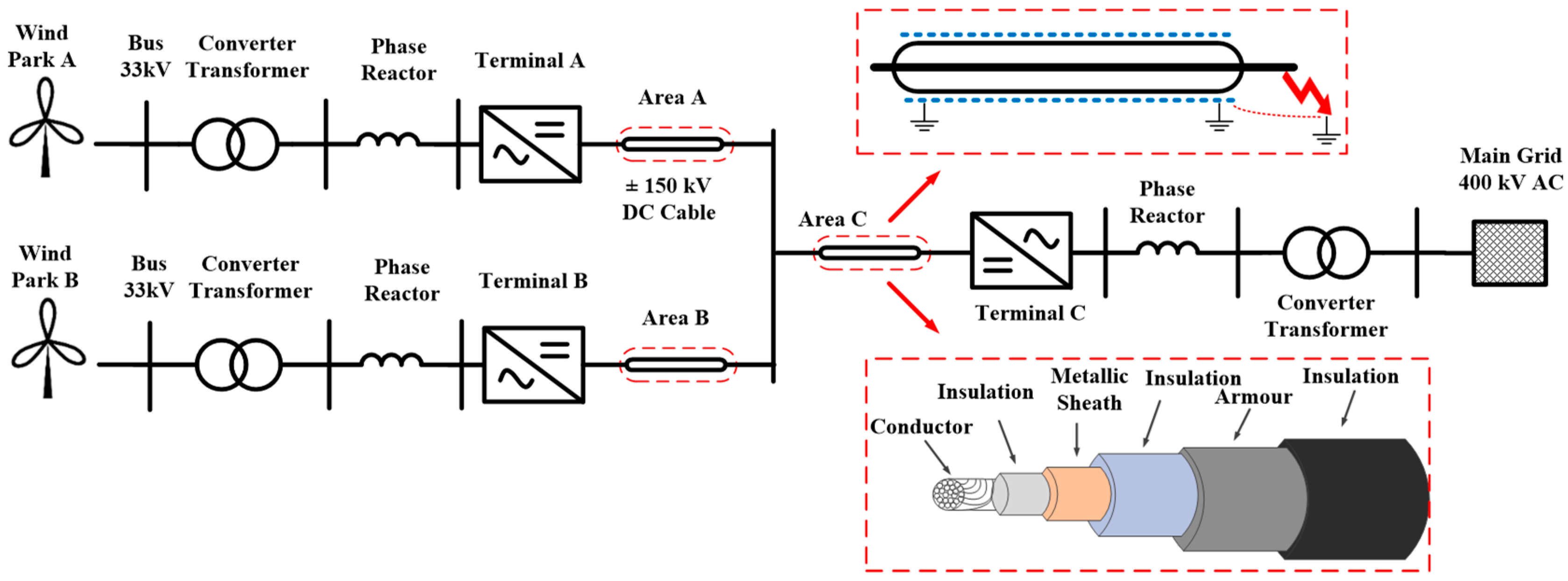
2. Transmission System of Multi-Terminal VSC-HVDC Connected to OWFs

The transmission system of multi-terminal VSC-HVDC connected to the OWFs usually includes multiple VSC units that are parallel connected via submarine HVDC cable.

2.1. Test System

As depicted in Figure 1, a multi-terminal HVDC system connected to OWF A and OWF B is utilized to be the test case [34]. To obtain the desired voltage level, a converter transformer is installed adjacent to each OWF. The system is equipped with a high-pass filter and series reactor to remove current harmonics. The generated electric power is transferred through the HVDC system to the main networks. The VSC control unit can independently adjust the phase angle and magnitude of AC voltage. In this way, the DC power and voltage on the AC side can be adjusted by phase angle and magnitude of generated voltage by the VSC. In [35,36], the topologies of two-level and three-level VSCs were investigated in detail. It has been shown that these topologies have similar transient behavior in DC fault conditions [13]. The midpoints of DC capacitors are grounded to remove the imbalance between positive and negative poles [35,36,37]. The reference voltage is also provided in bipolar HVDC systems. The cable sheath is grounded so that the fault current can return through the sheath, the grounded midpoint of the capacitor and the grounded link of the transformer [13]. However, with a suitable control strategy, the MMC could be more tolerable to DC faults.

2.2. DC Cable Fault Classification

The DC cable faults can be grouped into the following categories:
  • Positive cable ground fault.
  • Negative cable ground fault.
  • Pole-to-pole fault (positive cable to negative cable fault).
The pole-to-pole faults are very rare in submarine DC cables because positive and negative cables are separated by insulation and conduit sets. On the contrary, ground faults are very prevalent in DC submarine cables due to insulation breakdown because of cable aging and exposure to a wet environment.

3. The Proposed Concept

To present an effective fault location method, we need to review the transient behavior of the system under fault circumstances. During a severe DC cable fault in a multi-terminal system, the control unit of VSC blocks IGBTs rapidly by stopping the gate firing signal. Then, anti-parallel diodes act as uncontrolled rectifiers so that the fault current is fed from the AC side system [38]. The XLPE HVDC cable has a main conductor that is located at the center. Moreover, it has two conductive layers known as sheath and armor, which are separated by appropriate insulators. During normal conditions, the sheath current is zero. On the contrary, during fault conditions, the fault current passes through the sheath. Thus, the transient overvoltage appears and voltage surges travel from the fault location in both directions.
After a fault occurs in an HVDC link, the generated waves propagate through the main conductor and the cable sheath [39]. Thus, as an appropriate attribute, sheath voltage can be used for the fault location procedure. The extracted characteristics from the sheath voltage have the potential to be used in fault location estimation. This study investigated a combination of the mentioned characteristics with an artificial intelligence method i.e., an ANN, to locate DC faults. Sheath resistance has a direct relationship to fault distance from the intended terminal. Long-distance faults correspond to high sheath resistance. Therefore, the magnitude of the sheath voltage changes based on a change in fault distance. This means that the signal of the sheath voltage and possible features extracted from this signal can be appropriate criteria for fault location estimation in VSC-HVDC transmission systems.
Features extracted from the sheath voltage samples are given to the neural network as input data in the proposed algorithm. The input data have a vital role in the performance of the proposed method. A comprehensive investigation has been performed to extract the best features from the sampled data. With regard to the trend of the sheath voltage graph for different cases of DC fault and its characteristics, two appropriate features are selected:
  • Maximum absolute value of sampled data for sheath voltage (signal peak).
  • Average of sampled data for sheath voltage.
In this study, it is assumed that the fault detection process has been performed and a faulty branch identified. This can be achieved by detecting sudden changes in the magnitude of DC current and voltage in the related area. The faulty branch can also be diagnosed using the state of the DC circuit breaker of each area [7,8]. The open state of a DC circuit breaker means that a DC fault happened in that area. The algorithm to train and test the proposed method is shown in Figure 2. At first, the proposed method collects signals of sheath voltage measured at the HVDC cable terminals of three areas. Then, the calculation process of two features—the maximum absolute value and the average of sampled data—will be started. The proposed method will be trained by these features to achieve acceptable outputs. Finally, the trained ANN is able to estimate the fault location in the faulted area.

4. Simulation Results

Different simulations are performed in the PSCAD environment and are post-processed by MATLAB software to evaluate the performance of the suggested algorithm. A three-terminal multi-terminal VSC-HVDC system connected to two offshore wind farms is used as the case study, as depicted in Figure 1. The power generated by OWF A is 250 MW as OWF B generates 150 MW. The cable lengths in areas C, B and A are 100 km, 80 km and 60 km, respectively. Characteristics of the case study are shown in Table A1 in Appendix A. A frequency-dependent model of the cable is used in the case study using cable geometry features, resistivity, relative permittivity, and permeability of each section as input data [40,41]. The 150 kV cable parameters are shown in Table A2 in Appendix A.
A basic architecture of a three-layer feedforward ANN is shown in Figure 3. In this study, the feedforward–backpropagation type of the ANN has been used to locate DC faults in the HVDC cables. To train the neural network, 372 cases of faults have been tested on the HVDC cables of areas A, B and C. For each area, faults have been simulated at every 2.5 km on the length of each area cable. Both parameters of fault distance and resistance have been changed to run a variety of fault conditions. Each case of fault at a certain location has been simulated with fault resistance of 0 Ω, 10 Ω and 100 Ω. The sampling frequency of data measurement is set to 2.5 kHz. The length of the data window is one cycle, which is 20 ms for a power frequency of 50 Hz. In all cases, the measured voltages of the cable sheaths are given as inputs to the trained ANN. The output of the ANN is the distance to the fault point from the beginning of the faulted cable.
Different configurations are tested for the neural network and the best topology of the network is selected by trial-and-error process. The proposed network has three hidden layers with the neuron numbers 20, 30 and 10 for the first, second, and third layers, respectively. The output layer indicates the fault location on the cable of the faulted area. The optimized excitation functions for the first layer are set to piecewise linear function and for the second and third layers are set to sigmoid unipolar function. The back-error-propagation method selects random coefficients and weights for the ANN work nodes. Then, it feeds in an input pair and obtains the results. Afterward, the algorithm calculates the error at each node starting from the last stage and propagates the error backward. Then, it updates the values of the weights. This procedure is repeated with all input–output pairs defined in the training process. The procedure lasts until the network reaches the desired converging error. More details and equations of the ANN used in the simulation are given in Appendix B.
The following simulation results demonstrate that the neural network has good performance using these features. Figure 4 shows the results of the sheath voltages when a negative cable ground fault at a distance of 95 km happens in the area C. The sheath voltage of area C has the maximum magnitude. A fault case of the positive cable at a distance of 90 km from terminal C as is shown in Figure 5. Figure 4b and Figure 5a show that a fault at a shorter distance leads to a higher absolute value of signal peak for the sheath voltage and also signal average, as can be seen for the signal range in Figure 4b: between the times t = 5 s and t = 5.005 s, it is less than 1 kV, while it is more than 1 kV for the case in Figure 5a. The difference between peak values is related to the differences in fault distance of two cases. For the positive cable fault, only the positive sheath value is considered, while for the negative cable fault, only the negative sheath value is considered.
As an evaluation index, the estimation error is defined as follows:
Error (%) = ((Estimated location − Actual location)/Cable length) × 100

4.1. Simulation Results for Faults in Area A

Results of fault location estimation for positive cable in area A are shown in Table 1. Estimation errors for different cases of DC positive to ground fault are shown in the table. DC faults with different distances from the terminal A and resistances of 0 Ω, 10 Ω and 100 Ω are investigated. For example, the estimated error for the case of a DC fault at 30 km distance from the terminal A with a zero fault resistance is 0.27%. All of the cases have an estimated error of less than 1%. The maximum error is for the case of the fault at a distance of 40 km with fault resistance of 10 Ω, which is equal to 0.69%. The last row of the table shows the average of estimated error for the cases with certain fault resistance. As can be seen, the average error is increasing with an increase in fault resistance. Therefore, the cases with higher fault resistance are more challenging cases. Table 2 presents the outputs for negative cable ground faults of area A. The maximum error for these types of faults is 0.73%, which is for the case of a fault at a distance of 10 km with a resistance of 100 Ω. The trend of error average is similar to the positive cable faults in Table 1. Faults with resistance of 100 Ω have the maximum value for the estimated error average and faults with resistance of 0 Ω have the minimum value for the estimated average error. Generally, the results in Table 1 and Table 2 show the proposed method has good and reliable performance in area A.

4.2. Simulation Results for Faults in Area B

The results of the fault location for the positive cable in area B are shown in Table 3. For example, the estimated error for the case of a DC fault at 20 km distance from the terminal B with 10 Ω resistance is 0.31%. The maximum error is for the case of the fault at a distance of 60 km with a fault resistance of 10 Ω, which is equal to 0.77%. The averages of estimated error for the cases with fault resistances of 0 Ω, 10 Ω and 100 Ω are 0.420%, 0.484% and 0.594%, respectively. Table 4 presents the outputs for negative cable ground faults of the area B. The maximum error for these types of faults is 0.87%, which is for the case of a fault at a distance of 70 km with a resistance of 10 Ω. In this area, the amount of error average is increasing with an increase in fault resistance except in the cases of the negative cable faults with a resistance of 10 Ω. The estimated errors in Table 3 and Table 4 show the proposed method has robust performance in area B.

4.3. Simulation Results for Faults in Area C

Simulation results for faults in area C are shown in Table 5 and Table 6. The maximum error for positive cable faults is 0.88%, which is for the case of a fault at a distance of 70 km with a resistance of 100 Ω. The same case for negative cable faults has a maximum error of 0.80%. The averages of the estimated error for positive cable faults with fault resistance of 0 Ω, 10 Ω and 100 Ω are 0.447%, 0.515% and 0.655%, respectively. On the other hand, for negative cable faults, the averages of the estimated error for fault resistance of 0 Ω, 10 Ω and 100 Ω are 0.458%, 0.555% and 0.648%, respectively. Similar to the previous results in areas A and B, the averages of estimated error increase with an increase in fault resistance.
The simulation results for three areas of the case study demonstrate the suitable performance of the proposed algorithm. It can be seen from the tables that estimation errors for faults with high resistance are bigger than for low-resistance ones. The maximum estimated error for fault location in all studied cases of different areas belongs to area C, with the value of 0.88, which is less than 1%.
Moreover, a comparative assessment of the proposed fault location method with some fault location methods is shown in Table 7. As can be seen from the table, the proposed method has high accuracy and low sampling frequency in comparison with the existing fault location methods. Although the double-ended fault location methods have lower maximum error than the proposed method, they require communication links and data synchronization. Consequently, the cost of the required equipment is higher than the single-ended methods, including the proposed approach.

5. Conclusions

The use of multi-terminal VSC-HVDC transmission systems for large and integrated OWFs is increasing in modern power networks. One of the crucial aspects of studies in these kinds of systems is DC fault location. A new fault location method for the HVDC cable of a multi-terminal VSC system is presented in this paper. The proposed algorithm uses an ANN that is trained by special features extracted from the transient voltage of the cable sheath to exactly locate different DC faults. The combination of extracted features from the novel signal and the intelligent tool yields a new fault location method in the field of multi-terminal HVDC transmission systems. Varieties of fault conditions including negative and positive DC fault types with different locations and fault resistances are performed throughout the study. The simulation results show that the suggested method has reliable performance. Moreover, a comparison with existing methods has been presented in the last part of the study. The suggested method can provide the system with attractive advantages, such as lower sampling frequency, compared to the other methods.

Author Contributions

Conceptualization, S.H.A.N.; methodology, S.H.A.N.; software, S.H.A.N.; validation, S.H.A.N. and J.S.F.; resources, S.H.A.N. and J.S.F.; writing—original draft preparation, S.H.A.N.; writing—review and editing, S.H.A.N., J.S.F., Z.C. and B.B.-J.; supervision, Z.C., B.B.-J. and S.H. All authors have read and agreed to the published version of the manuscript.

Funding

This research was funded by the Sino-Danish Center (SDC) for Education and Research. Funding Number: 222519.

Institutional Review Board Statement

Not applicable.

Informed Consent Statement

Not applicable.

Data Availability Statement

Data are available on request from the corresponding author due to restrictions.

Conflicts of Interest

The authors declare no conflict of interest.

Appendix A

In this section, the parameters of the multi-terminal VSC-HVDC system and 150 kV XLPE cable are given in Table A1 and Table A2.
Table A1. The grid parameters.
ParametersValue
OWF power (in total)400 MW
Line-to-line AC voltage400 kV
Pole-to-ground DC voltage150 kV
X/R ratio (AC grid)10
Voltage ratio of VSC transformer33 kV/155 kV
Leakage reactance of converter transformer0.1 p.u.
DC capacitor100 µF
Table A2. The HVDC cable parameters.
Radius [m]Resistivity
(ohm*m)
Relative PermittivityRelative Permeability
Conductor0.0191.72 × 10−8-1
Main insulation0.039-2.5-
Sheath0.0422.2 × 10−7-1
Insulation A0.044-2.5-
Armor0.0491.8 × 10−7-100
Insulation B0.051-2.5-

Appendix B. More Details and Equations of the ANN Used in the Simulation Study

The ANN has the learning ability of exemplar patterns so that it can be used for both regression and classification purposes. This network consists of several layers: input, hidden, and output. Each layer has several neurons, and its output is considered as the next-layer input after passing through activation function. The activation function can be linear, hyperbolic, and tangential. The layers’ connection is established through a weight matrix. In order to recognize the nonlinear and complicated relationship between input and output matrices, the bias vector and weight matrix should be determined so that the maximum estimation accuracy is obtained. To achieve this goal, the weight and bias are gradated in a repetitive process based on the gradient descent method. Assuming that the connecting weight between neuron i and j is wij and neuron bias is bi, then the output of the ith neuron is expressed as follows:
x i = f ξ i
ξ i = j Γ i 1 w i j x j + b i
where Γ i 1 is a set of connected neurons to the ith neuron in the previous layer. In order to adjust the bias and weight, the backpropagation method is utilized based on the gradient descent as follows:
w i j k + 1 = w i j k λ E w i j k
b i j k + 1 = b i j k λ E b i j k
where λ is the learning rate and E is calculated as below:
E = 1 2 x o x ^ o 2
where x o is the calculated output vector and x ^ o is the desired target vector. The error derivative with respect to weight and bias of the ith neuron is calculated as follows:
E w i j = E x i f ξ i x j
E b i = E x i f ξ i
As such, we have:
E w i j = E b i x j
If the neuron i belongs to the output layer:
E x i = x o x ^ o
and if the neuron i belongs to the hidden layer:
E x i = l Γ i E x l f ξ i w l i = l Γ i E b i w l i
where Γ i is a set of connected neurons to the ith neuron in the next layer. As can be found from (10), for the calculation of the error derivate of each neuron with respect to its inputs, the error derivate should first be calculated for neurons of the next layer. As such, in order to adjust the bias and weight, the output layer error should be calculated according to (9) and then the error derivative for hidden layers neuron is calculated as (10). This process can be repeated for a predetermined number or desirable error.

References

  1. Morton, A.B.; Cowdroy, S.; Hill, J.R.A.; Halliday, M.; Nicholson, G.D. AC or dc economics of grid connection design for offshore wind farms. In Proceedings of the IEE International Conference on AC-DC Power Transmission (ACDC 2006), London, UK, 28–31 March 2006; pp. 236–240. [Google Scholar]
  2. Bresesti, P.; Kling, W.L.; Hendriks, R.L.; Vailati, R. HVDC Connection of Offshore Wind Farms to the Transmission System. IEEE Trans. Energy Convers. 2007, 22, 37–43. [Google Scholar] [CrossRef]
  3. Kirby, N.; Xu, L.; Luckett, M.; Siepmann, W. HVDC transmission for large offshore wind farms. Power Eng. 2002, 16, 135–141. [Google Scholar] [CrossRef]
  4. Koldby, E.; Hyttinen, M. Challenges on the Road to an Offshore HVDC Grid. In Proceedings of the Nordic Wind Power Conference, Bornholm, Denmark, 10–11 September 2009. [Google Scholar]
  5. Schettler, F.; Huang, H.; Christl, N. HVDC transmission systems using voltage sourced converters design and applications. In Proceedings of the 2000 Power Engineering Society Summer Meeting, Seattle, WA, USA, 16–20 July 2000; Volume 2, pp. 715–720. [Google Scholar]
  6. Tang, L.; Wu, B.; Yaramasu, V.; Chen, W.; Athab, H.S. Novel dc/dc choppers with circuit breaker functionality for HVDC transmission lines. Electr. Power Syst. Res. 2014, 116, 106–116. [Google Scholar] [CrossRef]
  7. Rakhshani, E.; Remon, D.; Rodriguez, P. Effects of PLL and frequency measurements on LFC problem in multi-area HVDC interconnected systems. Int. J. Electr. Power Energy Syst. 2016, 81, 140–152. [Google Scholar] [CrossRef]
  8. Yang, B.; Sang, Y.; Shi, K.; Yao, W.; Jiang, L.; Yu, T. Design and real-time implementation of perturbation observer based sliding-mode control for VSC-HVDC systems. Control Eng. Pract. 2016, 56, 13–26. [Google Scholar] [CrossRef]
  9. Dirk Van Hertem, O.G.-B.; Liang, J. HVDC Grids: For Offshore and Supergrid of the Future; IEEE Press Series on Power Engineering; John Wiley & Sons: Hoboken, NJ, USA, 2016. [Google Scholar]
  10. Sano, K.; Takasaki, M. A Surgeless Solid-State DC Circuit Breaker for Voltage-Source-Converter-Based HVDC Systems. IEEE Trans. Ind. Appl. 2013, 50, 2690–2699. [Google Scholar] [CrossRef]
  11. Tang, L.; Ooi, B.T. Protection of VSC-multi-terminal HVDC against DC faults. In Proceedings of the 2002 IEEE 33rd Annual IEEE Power Electronics Specialists Conference, Cairns, Australia, 23–27 June 2002; pp. 719–724. [Google Scholar]
  12. Yang, J.; Fletcher, J.E.; O’Reilly, J. Multiterminal dc wind farm collection grid internal fault analysis and protection scheme design. IEEE Trans. Power Deliv. 2010, 25, 2308–2318. [Google Scholar] [CrossRef]
  13. Tang, L.; Ooi, B.-T. Locating and Isolating DC Faults in Multi-Terminal DC Systems. IEEE Trans. Power Deliv. 2007, 22, 1877–1884. [Google Scholar] [CrossRef]
  14. Kwon, Y.-J.; Kang, S.-H.; Lee, D.-G.; Kim, H.-K. Fault location algorithm based on cross correlation method for HVDC cable lines. In Proceedings of the IET 9th International Conference Developments in Power System Protection, Glasgow, UK, 17–20 March 2008; pp. 17–20. [Google Scholar]
  15. Pan, Y.; Steurer, M.; Baldwin, T. Feasibility study of noise pattern analysis based ground fault locating method for ungrounded dc shipboard power distribution systems. In Proceedings of the 2009 IEEE Electric Ship Technologies Symposium ESTS, Baltimore, MD, USA, 20–22 April 2009; IEEE: Piscataway, NJ, USA, 2009. [Google Scholar]
  16. Christopher, E.; Sumner, M.; Thomas, D.W.; Wang, X.; de Wildt, F. Fault location in a zonal DC marine power system using active impedance estimation. In Proceedings of the Energy Conversion Congress and Exposition (ECCE), Atlanta, GA, USA, 12–16 September 2010. [Google Scholar]
  17. Kwon, Y.J.; Kang, S.H.; Choi, C.Y.; Ji, S.Y. A Fault Location Algorithm for VSC HVDC Cable lines. In Proceedings of the International Conference on Electrical Engineering, ICEE, Krabi, Thailand, 14–17 May 2008. [Google Scholar]
  18. Yang, J.; Fletcher, J.E.; O’Reilly, J. Short-circuit and ground fault analysis and location in VSC-based DC network cables. IEEE Trans. Ind. Electron. 2012, 59, 3827–3837. [Google Scholar] [CrossRef]
  19. Leterme, W.; Azad, S.P.; Van Hertem, D. HVDC grid protection algorithm design in phase and modal domains. IET Renew. Power Gener. 2018, 12, 1538–1546. [Google Scholar] [CrossRef]
  20. Jia, K.; Chen, R.; Xuan, Z.; Yang, Z.; Fang, Y.; Bi, T. Fault characteristics and protection adaptability analysis in VSC-HVDC-connected offshore wind farm integration system. IET Renew. Power Gener. 2018, 12, 1547–1554. [Google Scholar] [CrossRef]
  21. Marvasti, F.D.; Mirzaei, A. A Novel Method of Combined DC and Harmonic Overcurrent Protection for Rectifier Converters of Monopolar HVDC Systems. IEEE Trans. Power Deliv. 2018, 33, 892–900. [Google Scholar] [CrossRef]
  22. Leterme, W.; Hertem, D.V. Cable Protection in HVDC Grids Employing Distributed Sensors and Proactive HVDC Breakers. IEEE Trans. Power Deliv. 2018, 33, 1981–1990. [Google Scholar] [CrossRef]
  23. Ma, Y.; Li, H.; Wang, G.; Wu, J. Fault Analysis and Traveling-Wave-Based Protection Scheme for Double-Circuit LCC-HVDC Transmission Lines with Shared Towers. IEEE Trans. Power Deliv. 2018, 33, 1479–1488. [Google Scholar] [CrossRef]
  24. Nanayakkara, O.M.K.K.; Rajapakse, A.D.; Wachal, R. Traveling-Wave-Based Line Fault Location in Star-Connected Multiterminal HVDC Systems. IEEE Trans. Power Deliv. 2012, 27, 2286–2294. [Google Scholar] [CrossRef]
  25. Gao, S.-P.; Chu, X.; Shen, Q.-Y.; Jin, X.-F.; Luo, J.; Yun, Y.-Y.; Song, G.-B. A novel whole-line quick-action protection principle for HVDC transmission lines using one-end voltage. Int. J. Electr. Power Energy Syst. 2015, 65, 262–270. [Google Scholar] [CrossRef]
  26. Nanayakkara, O.M.K.K.; Rajapakse, A.D.; Wachal, R. Location of DC Line Faults in Conventional HVDC Systems with Segments of Cables and Overhead Lines Using Terminal Measurements. IEEE Trans. Power Deliv. 2011, 27, 279–288. [Google Scholar] [CrossRef]
  27. De Kerf, K.; Srivastava, K.; Reza, M.; Bekaert, D.; Cole, S.; Van Hertem, D.; Belmans, R. Wavelet-based protection strategy for DC faults in multi-terminal VSC HVDC systems. IET Gener. Transm. Distrib. 2011, 5, 496–503. [Google Scholar] [CrossRef]
  28. Liu, X.; Osman, A.H.; Malik, O.P. Hybrid Traveling Wave/Boundary Protection for Monopolar HVDC Line. IEEE Trans. Power Deliv. 2009, 24, 569–578. [Google Scholar] [CrossRef]
  29. Xiao-Dong, Z.; Neng-Ling, T.; Thorp, J.S.; Guang-Liang, Y. A transient harmonic current protection scheme for HVDC transmission line. IEEE Trans. Power Deliv. 2012, 27, 2278–2285. [Google Scholar]
  30. Zheng, J.; Wen, M.; Chen, Y.; Shao, X. A novel differential protection scheme for HVDC transmission lines. Int. J. Electr. Power Energy Syst. 2018, 94, 171–178. [Google Scholar] [CrossRef]
  31. Farshad, M.; Sadeh, J. A Novel Fault-Location Method for HVDC Transmission Lines Based on Similarity Measure of Voltage Signals. IEEE Trans. Power Deliv. 2013, 28, 2483–2490. [Google Scholar] [CrossRef]
  32. He, Z.-Y.; Liao, K.; Li, X.-P.; Lin, S.; Yang, J.-W.; Mai, R.-K. Natural Frequency-Based Line Fault Location in HVDC Lines. IEEE Trans. Power Deliv. 2013, 29, 851–859. [Google Scholar] [CrossRef]
  33. Hao, Y.; Wang, Q.; Li, Y.; Song, W. An intelligent algorithm for fault location on VSC-HVDC system. Int. J. Electr. Power Energy Syst. 2018, 94, 116–123. [Google Scholar] [CrossRef]
  34. Liang, J.; Jing, T.; Gomis-Bellmunt, O.; Ekanayake, J.; Jenkins, N. Operation and Control of Multiterminal HVDC Transmission for Offshore Wind Farms. IEEE Trans. Power Deliv. 2011, 26, 2596–2604. [Google Scholar] [CrossRef]
  35. Bahrman, M.P.; Johnson, B.K. The ABCs of HVDC transmission technologies. IEEE Power Energy Mag. 2007, 5, 32–44. [Google Scholar] [CrossRef]
  36. Baran, M.; Mahajan, N. DC distribution for industrial systems: Opportunities and challenges. IEEE Trans. Ind. Appl. 2003, 39, 1596–1601. [Google Scholar] [CrossRef]
  37. Nguefeu, S.; Rault, P.; Grieshaber, W.; Hassan, F. DEMO 3 Requirement Specifications: Detailed Specifications for a DC Network and Detailed Specifications for ALSTOM Grid’s DC Breaker. Deliverable n°11.1 of the Twenties Project. 2012. Available online: http://www.twentiesproject.eu/node/18 (accessed on 1 January 2014).
  38. Bucher, M.K.; Franck, C.M. Contribution of Fault Current Sources in Multiterminal HVDC Cable Networks. IEEE Trans. Power Deliv. 2013, 28, 1796–1803. [Google Scholar] [CrossRef]
  39. Ashrafi Niaki, S.H.; Liu, Z.; Chen, Z.; Bak-Jensen, B.; Hu, S. Protection System of Multi-Terminal MMC-based HVDC Grids: A Survey. In Proceedings of the 2022 International Conference on Power Energy Systems and Applications (ICoPESA), Singapore, 25–27 February 2022; pp. 167–177. [Google Scholar]
  40. Marti, J. Accurate modeling of frequency dependent transmission lines in electromagnetic transients simulation. IEEE Trans. Power Appar. Syst. 1982, 101, 147–155. [Google Scholar] [CrossRef]
  41. Morched, A.; Gustavsen, B.; Tartibi, M. A universal model for accurate calculation of electromagnetic transients on overhead lines and underground cables. IEEE Trans. Power Deliv. 1999, 14, 1032–1038. [Google Scholar] [CrossRef]
  42. Suonan, J.; Gao, S.; Song, G.; Jiao, Z.; Kang, X. A Novel Fault-Location Method for HVDC Transmission Lines. IEEE Trans. Power Deliv. 2009, 25, 1203–1209. [Google Scholar] [CrossRef]
  43. Fayazi, M.; Joorabian, M.; Saffarian, A.; Monadi, M. A single-ended traveling wave based fault location method using DWT in hybrid parallel HVAC/HVDC overhead transmission lines on the same tower. Electr. Power Syst. Res. 2023, 220, 109302. [Google Scholar] [CrossRef]
  44. Zhang, X.; Tai, N.; Zheng, X.; Huang, W. Wavelet-based EMTR method for fault location of VSC-HVDC transmission lines. J. Eng. 2019, 2019, 961–966. [Google Scholar] [CrossRef]
  45. Farshad, M.; Karimi, M. A Signal Segmentation Approach to Identify Incident/Reflected Traveling Waves for Fault Location in Half-Bridge MMC-HVdc Grids. IEEE Trans. Instrum. Meas. 2021, 71, 1–9. [Google Scholar] [CrossRef]
  46. Suonan, J.; Zhang, J.; Jiao, Z.; Yang, L.; Song, G. Distance Protection for HVDC Transmission Lines Considering Frequency-Dependent Parameters. IEEE Trans. Power Deliv. 2013, 28, 723–732. [Google Scholar] [CrossRef]
  47. Luo, G.; Yao, C.; Liu, Y.; Tan, Y.; He, J.; Wang, K. Stacked Auto-Encoder Based Fault Location in VSC-HVDC. IEEE Access 2018, 6, 33216–33224. [Google Scholar] [CrossRef]
  48. Silva, A.S.; Santos, R.C.; Torres, J.A.; Coury, D.V. An accurate method for fault location in HVDC systems based on pattern recognition of DC voltage signals. Electr. Power Syst. Res. 2019, 170, 64–71. [Google Scholar] [CrossRef]
Figure 1. Case study.
Wind 03 00021 g001
Figure 2. The proposed algorithm.
Wind 03 00021 g002
Figure 3. A basic architecture of a three-layer feedforward ANN.
Wind 03 00021 g003
Figure 4. Signals of sheath voltage when the negative cable to ground fault happens at 95 km distance: (a) positive cable (b) negative cable.
Wind 03 00021 g004
Figure 5. Signals of sheath voltage when the positive cable to ground fault happens at 90 km distance: (a) positive cable (b) negative cable.
Wind 03 00021 g005
Table 1. Results of fault location estimation for the positive cable of area A.
Fault Distance
(km)
Fault Resistance (Ω)Mean Absolute Error (%)
010100
Estimation Error (%)
100.330.490.530.45
200.650.320.400.456
300.270.380.390.346
400.420.690.580.563
500.290.480.630.466
Estimated Error Average0.3920.4720.5060.4562
Table 2. Fault location results for the negative cable of area A.
Fault Distance
(km)
Fault Resistance (Ω)Mean Absolute Error (%)
010100
Estimation Error (%)
100.450.410.730.53
200.550.370.460.46
300.160.440.640.413
400.520.600.710.61
500.210.400.590.4
Estimated Error Average0.3780.4440.6260.4826
Table 3. Results of fault location estimation for the positive cable in area B.
Fault Distance
(km)
Fault Resistance (Ω)Mean Absolute Error (%)
010100
Estimation Error (%)
100.130.220.440.263
200.320.310.640.423
300.540.660.600.6
400.370.510.750.453
500.740.530.550.606
600.360.770.610.58
700.480.390.570.48
Estimated Error Average0.4200.4840.5940.486
Table 4. Results of fault location estimation for the negative cable in area B.
Fault Distance
(km)
Fault Resistance (Ω)Mean Absolute Error (%)
010100
Estimation Error (%)
100.170.640.490.433
200.560.850.550.653
300.500.520.600.54
400.470.300.730.5
500.640.740.670.683
600.300.310.530.38
700.710.870.500.693
Estimated Error Average0.4780.6040.5810.554
Table 5. Result of fault location estimation for the positive cable of area C.
Fault Distance
(km)
Fault Resistance (Ω)Mean Absolute Error (%)
010100
Estimation Error (%)
100.500.420.540.486
200.110.310.430.283
300.440.480.590.503
400.570.660.850.693
500.360.500.730.53
600.410.310.600.44
700.480.630.880.663
800.570.620.550.58
900.590.710.730.676
Estimated Error Average0.4470.5150.6550.539
Table 6. Results of fault location estimation for the negative cable of area C.
Fault Distance
(km)
Fault Resistance (Ω)Mean Absolute Error (%)
010100
Estimation Error (%)
100.520.790.500.603
200.250.210.620.36
300.340.430.510.426
400.640.690.740.69
500.300.680.790.59
600.480.550.660.563
700.430.630.800.62
800.500.420.450.456
900.670.600.770.68
Estimated Error Average0.4580.5550.6480.554
Table 7. Comparative analysis of the proposed fault location with existing methods.
ReferenceAlgorithmSignal UsedSampling Frequency
(kHz)
Communication
Required
Max. Error (%)
[42]Voltage distributionCurrent and voltage100 Yes (double-ended)0.78
[43]DWT *Voltage 100No (single-ended)0.85
[44]WaveletCurrent50–200Yes (double-ended)0.965
[45]SSA *Voltage 250No (single-ended)2.12
[46]Distance
relay
Current and voltage80No (single-ended)3.6
[47]SAE *Current5No (single-ended)1.23
[48]ANNVoltage20No (single-ended)5.69
Proposed methodANNSheath voltage2.5No (single-ended)0.88
* Discrete Wavelet (DWT), Signal segmentation approach (SSA), Stacked auto-encoder (SAE).
Disclaimer/Publisher’s Note: The statements, opinions and data contained in all publications are solely those of the individual author(s) and contributor(s) and not of MDPI and/or the editor(s). MDPI and/or the editor(s) disclaim responsibility for any injury to people or property resulting from any ideas, methods, instructions or products referred to in the content.

