Abstract
The present research explores the optimization of maintenance strategies for floating offshore wind (FOW) farms using nested genetic algorithms. The primary goal is to provide insights on the decision-making processes required for both immediate and strategic maintenance planning, crucial for the viability and efficiency of FOW operations. A nested genetic algorithm was coupled with discrete-event simulations in order to simulate and optimize maintenance scenarios influenced by various operational and environmental parameters. The study revealed that short-term maintenance timing is significantly influenced by wind conditions, with higher electricity prices justifying on-site spare parts storage to mitigate operational disruptions, suggesting economic incentives for maintaining on-site inventory of spare parts. Long-term strategic findings emphasized the impact of planned intervals between inspections on financial outcomes, identifying optimal strategies that balance operational costs with energy production efficiency. Ultimately, this study highlights the importance of integrating sophisticated predictive models for failure detection with real-time operational data to enhance maintenance decision-making in the evolving landscape of offshore wind energy, where future farms are likely to operate farther from onshore facilities and under potentially highly varying market conditions in terms of electricity prices.
1. Introduction
The market of global offshore wind (OSW) is evolving fast and changing continuously because of the rise in installed capacity and falling implementation costs [1]. A critical development in this field is related to floating offshore wind (FOW) technologies, which will enable harnessing of wind energy resources in deeper waters, where it would have been uneconomic to use traditional fixed-bottom turbines before. In 2023, the Global Wind Energy Council updated its 2030 forecast of installed offshore wind capacity to 316 GW, from which 19 GW are estimated for floating farms [2]. This trend is currently being witnessed with the continuous licensing and deployment of bigger floating wind farms, with larger turbines, which is pushing these technologies to higher technology readiness levels [3].
Portugal and the USA are leading key promoters pushing the development of FOW technologies, considering their offshore areas are suited for these technologies. Portugal has been acting as an innovation sandbox for FOW: innovative projects such as the WindFloat introduced the country to its strong potential for offshore wind [4]. Building on the potentials of the extensive ocean area of the country, the government launched a National Plan to establish the framework for public policy within Energy and Climate up to 2030 (Diário da República Portuguesa, 2020). This plan predicts the implementation of 2 GW of offshore wind capacity by 2030 and 10 GW by 2040—mostly, if not all, using floating solutions [5]. On the other hand, the United States is positioned to tap its offshore wind potential in deep-water areas, notably along its West Coast and in the Gulf of Maine. The U.S. has recently announced the Floating Offshore Wind Shot initiative, which aims to implement 110 GW of capacity installed in federal waters by 2050. Before that, by 2035, the Department of Energy is expecting big cost drops for FOW, which may hopefully support the deployment of 15 GW of floating offshore wind capacity by then—enough to power over five million homes. This initiative presents a significant step towards the intention of positioning the U.S. as the leader in the global FOW market [6].
Unlike bottom-fixed turbines that are anchored directly to the seabed, FOW turbines are installed on floating platforms, usually moored and anchored to the seabed but inherently influenced by the ocean’s currents and waves. This dynamic character introduces additional complexities during maintenance operations, as it requires innovative technical strategies to ensure the turbines remain operational despite the harsh marine conditions. Currently, the industry is considering two primary strategies for large-scale FOW maintenance:
- Tow-to-Port Maintenance: This strategy involves disconnecting the floating turbines from their moorings and towing them to a port or shipyard. Once ashore, maintenance operations or upgrades can be conducted within a controlled environment. This approach is particularly advantageous for major overhauls or when the required maintenance cannot be safely or effectively performed at sea [7].
- In Situ Maintenance: Based on specialized cranes, in situ maintenance may be carried out directly on the floating platforms at their operational site. This strategy is being designed for routine maintenance tasks, minor repairs, or even replacement of big components, including the generator and the blades. Nonetheless, these innovative cranes are still under development, thus leaving tow-to-port as the only viable maintenance strategy for FOW, as of today [8].
Furthermore, the implementation of adequate maintenance decisions is critical for ensuring both the immediate functionality and long-term viability of these floating farms. These decisions are divided into short-term and long-term strategies, each vital for different aspects of wind farm management:
- Tactical Short-term Maintenance Decisions are primarily concerned with immediate, often reactive, measures to address failures and routine maintenance tasks. These actions, including quick fixes, minor repairs, and regular inspections, are essential for minimizing downtime and ensuring uninterrupted energy production.
- Strategic Long-term Maintenance Decisions, on the other hand, encompass a broader scope of planning and foresight. This includes the adoption of advanced predictive maintenance technologies, strategic replacement of critical components before the end of their lifecycle, and major upgrades to enhance operational efficiency and adapt to evolving technologies. These decisions are informed by data analytics, trend analysis, and risk assessment to preemptively address potential issues, optimize the lifespan of the wind farm, and align with future technological advancements and regulatory requirements. Strategic long-term planning is essential for sustainable operation, aiming to reduce overall maintenance costs, improve reliability, and ensure the wind farm’s competitiveness in the energy market.
The interdependence between short-term and long-term strategies highlights the importance of a holistic approach to maintenance planning. Effective integration of both strategies ensures that short-term repairs align with broader operational goals, thereby enhancing the overall sustainability and profitability of the analyzed wind farm [9]. Recent studies, such as Zhao et al. (2023), emphasize the effectiveness of failure prediction and preventive maintenance strategies in enhancing the reliability of floating offshore wind turbine generators, supporting the importance of sophisticated maintenance frameworks [10]. Miguel de Matos Sá et al. [11] have evaluated the influence of weather forecast uncertainty and wake losses on the operational profitability of floating OSW farms. Similar models have been proposed by other authors for maintenance optimization and decision support for marine renewable farms [12,13], but they are not usually coupled with evolutionary algorithms, which often leads to their inability to efficiently navigate the vast solution spaces due to reliance on heuristic or gradient-based methods and their potential computational impracticality when faced with the exhaustive exploration of all possible solutions. To improve solution space navigation, genetic algorithms (GAs) offer a powerful tool for actively searching for solutions that promote the enhancement of maintenance schedules, component replacements, and logistics [14], as they simulate natural selection, identifying the most effective solutions based on various factors, such as weather conditions, turbine data, and crew availability, amongst others [15,16].
This study seeks to advance maintenance decision-making for floating offshore wind (FOW) installations by integrating nested genetic algorithms and discrete-event simulations, techniques not previously applied together in this context. By using the tow-to-port strategy as a baseline, this research introduces the application of genetic algorithms (GAs) to refine maintenance planning processes. This strategy allows for data-driven, computationally efficient decision-making that enhances both short-term readiness and long-term scheduling. Utilizing the Windfloat Atlantic wind farm as a case study provides practical insights from a pioneering FOW project, demonstrating how these advanced techniques can be applied to optimize maintenance strategies amongst the evolving demands of FOW operations.
2. Methods
The optimization of spare-part logistics and maintenance scheduling constitutes a fundamental challenge in the management of floating offshore wind (FOW) farms. This research introduces a model designed to explore the complexities of this industrial problem, providing a robust framework for decision-making. Integral to the model’s conception is the acknowledgment of the holistic nature of spare part distribution, which is influenced by fluctuating economic conditions, such as price indices and industry demand. These factors, coupled with the critical need for timely part delivery to prevent turbine downtime, add layers of complexity to the logistics process.
2.1. Problem Statement
The model implemented in this research aims to optimize spare-part logistics and maintenance decisions within a network of geographically distributed offshore wind turbines.
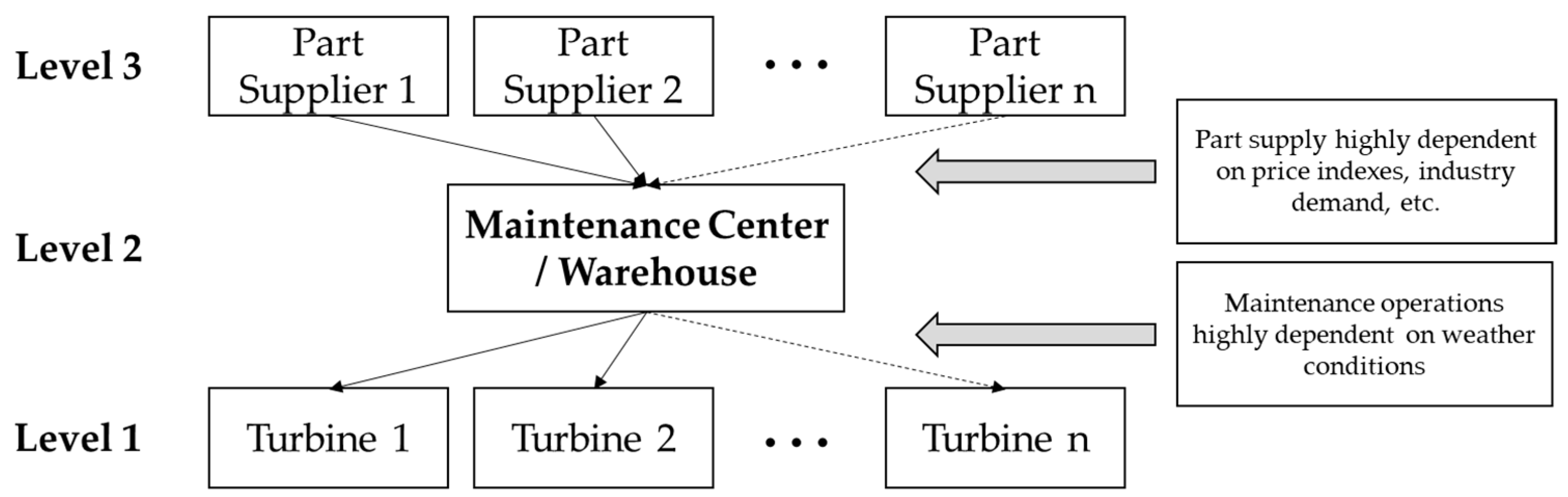
The logistics of spare parts are intrinsically complex due to several factors, prominently including the stochastic nature of part failures and the subsequent need for replacements. As depicted in Figure 1, the model developed under this research centralizes its analysis on a maintenance center/warehouse (fed by different geographically distributed part suppliers) and the respective connections to multiple offshore turbines. These connections are not merely physical but also temporal, with routes from parts suppliers to maintenance centers and turbines being quantified in hours.
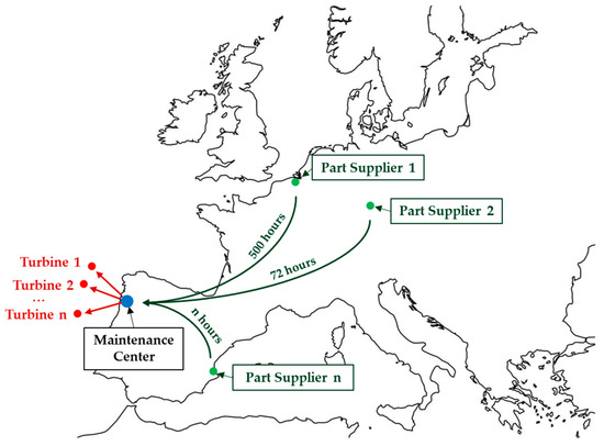
Figure 1.
Generic schematization of the interdependencies between part suppliers, maintenance centers, and the maintenance procedures of floating offshore wind turbines.
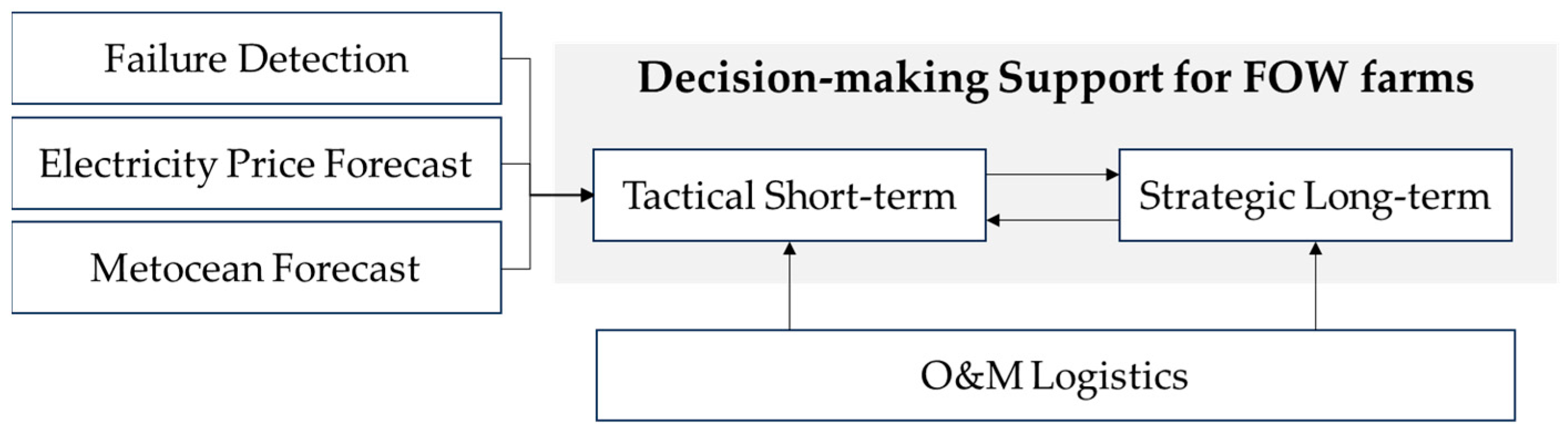
In Figure 2, two significant dependencies under the proposed framework are highlighted: the unpredictable nature of part supply, which is contingent on factors like price indices and industry demand, and maintenance operations, which are greatly influenced by weather conditions. These dependencies underscore the complexity of the model, which must account for these uncertainties through its optimization equations and the respective variables assumed.

Figure 2.
Depiction of the three-level framework implemented under the present research.
As stated, maintenance operations within FOW farms are heavily contingent upon variable and often adverse weather conditions, which can significantly disrupt planned activities. The proposed model incorporates a dynamic approach to maintenance scheduling that is sensitive to these environmental uncertainties. By integrating the influence of meteorological data, the model is capable of adapting maintenance strategies to improve the timing and execution of operations.
The architecture of the proposed model is modular, encompassing independent yet interrelated components that handle various operational aspects of the maintenance process. These modules, responsible for predicting failures, predicting electricity prices, and forecasting metocean conditions, collectively inform a layered decision-making framework. This framework, schematically presented in Figure 3, distinguishes between tactical short-term actions, which respond to immediate operational needs, and strategic long-term planning, which shapes the broader scope of maintenance strategies.
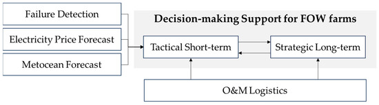
Figure 3.
Modular architecture of the model proposed under the present research.
The hypotheses of the model are grounded in the challenges faced by floating offshore wind farms. These turbines operate under harsh environmental conditions, and the supply chain for spare parts stretches across vast distances, complicating the logistics and elevating the risk of extended downtimes:
- Temporal flexibility in maintenance scheduling: The model assumes that maintenance activities can be scheduled flexibly over short-term and long-term periods. The use of nested GAs allows the interaction between these two temporal dimensions. By analyzing both short-term and long-term spectra and considering their mutual influences, the model hypothesizes that decisions made in one timeframe have significant implications for the other.
- Predictive maintenance capability: The model operates under the hypothesis that maintenance needs can be anticipated through the analysis of operational data. This is incorporated through component condition thresholds intervals between inspections as variables, seeking to preempt maintenance issues before they lead to component failure.
- Impact of Maintenance on Energy Production and Revenue: The model hypothesizes that maintenance operations have a direct impact on the energy production efficiency of FOW farms; furthermore, it takes into consideration the electricity price forecast to propose the execution of maintenance procedures during periods of lower electricity market prices.
- Operational and Environmental Constraints: The inclusion of variables such as weather conditions and logistic considerations (e.g., availability of vessels for tow-to-port operations and the existence of spare parts at the maintenance center) implies that the implemented modeling of the operational efficiency of FOW farms is heavily influenced by environmental conditions and logistical factors.
As any model that simulates a certain reality, the proposed model has some limitations that need to be acknowledged:
- Data Dependence: The model relies heavily on the quality and availability of input data, such as accurate failure detection, electricity price forecasts, and metocean forecasts. If these data are incomplete, inaccurate, or outdated, the model’s outputs will be compromised.
- Environmental and Regulatory Changes: Environmental policies and regulations impacting O&M activities in FOW farms are subject to change, which may not be fully accounted for in a model that is based on current standards and practices.
- Cost Model Simplifications: The model simplifies the complex cost structures associated with maintenance activities of OSW farms, which could potentially overlook factors such as varying labor costs, penalties for downtime, and the financial impact of unexpected delays.
- Interaction Effects: The model considers the interdependencies between short-term and long-term maintenance decisions. However, capturing the full spectrum of interaction effects accurately is challenging and may not reflect all the complexities of real-world operations.
- Complexity in Real-World Application: While the model may perform well under simulated or controlled conditions, translating its recommendations into practical, real-world FOW farm management involves logistical complexities and may encounter unforeseen implementation challenges.
Acknowledging its limitations, the model is intentionally designed with modularity to ensure flexibility and ease of updates. To put the developed model up to test, the present research will use as case study the Windfloat Atlantic floating OSW farm—as partially revealed in Figure 1. This farm, implemented off the north coast of Portugal back in 2019, was one of the first grid-connected farms of its kind. It is a pre-commercial 3-turbine farm—from the manufacturer Vestas, with a total output of 25 MW—and is expected to operate for the next 25 years. Its pioneering status as a pre-commercial venture offers valuable insights into the unique challenges and opportunities of floating OSW farms, making it an exemplary testbed for the model’s strategic maintenance optimization features.
2.2. Decision-Making Support Module
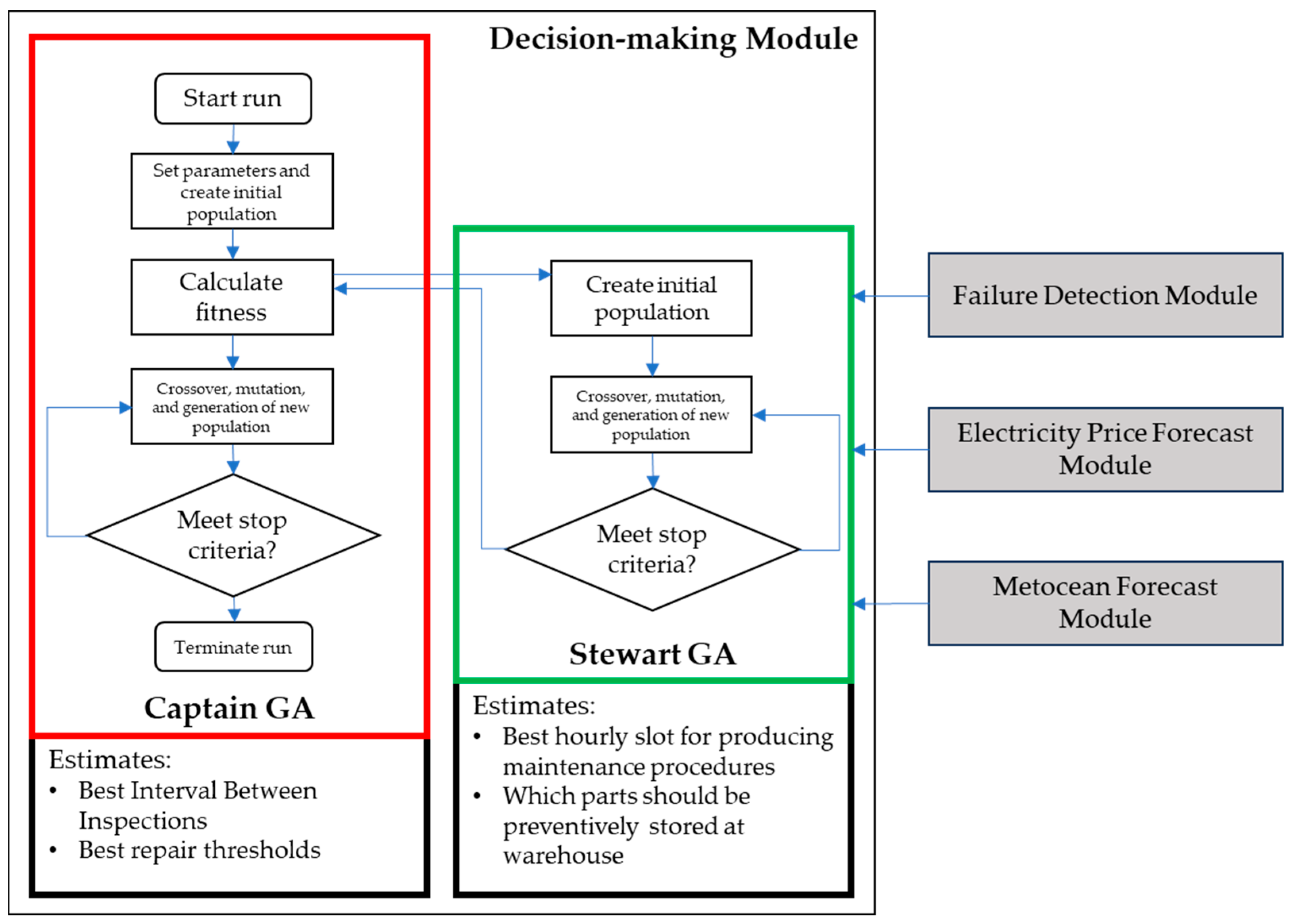
A nested GA framework is developed under this research to address the complex and interdependent decision-making processes in OSW farm maintenance. The traditional GA-based approach is expanded into a nested structure to capture the interplay between short-term operational decisions and long-term strategic planning. The developed model is built within the Python environment, leveraging the DEAP (Distributed Evolutionary Algorithms in Python) library [17]. The DEAP library provides a versatile toolbox for evolutionary computation, enabling the implementation of complex genetic operations such as mutation, crossover, and gene correction within a constraint optimization context.
For the outer layer, known as the “Captain GA”, the ‘eaMuPlusLambda’ evolutionary strategy is employed, which uses a combination of the best individuals (µ) and the offspring (λ) to create a new generation, thereby maintaining elite solutions while encouraging diverse exploratory steps through crossover and mutation [17]. This approach promotes robust search capability within the solution space and is particularly effective when contending with the stochastic nature of the failure models in OSW farms.
Within the proposed framework, schematically shown in Figure 4, the inner GA, also referred to as “Stewart GA”, is dedicated to optimizing immediate maintenance activities that are sensitive to operational exigencies and rapidly changing environmental and meteorological conditions. The resulting decisions are then integrated as parameters into the outer GA, referred to as the “Captain GA”, which is tasked with improving strategic maintenance parameters that secure long-term operational efficiency and farm viability.
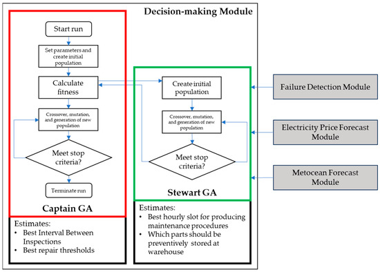
Figure 4.
Detailed schematic of the nested algorithm logic implemented, with the Captain GA simulating long-term strategic parameters and the Stewart GA testing out short-term tactical insights for maintenance actions.
For both the “Captain GA” (outer layer) and the “Stewart GA” (inner layer), the ‘eaMuPlusLambda’ algorithm was utilized. The GAs implemented within this framework are also characterized by the additional features:
- Mutation: This operation integrates randomness into the gene pool, creating opportunities for novel solutions to arise.
- Crossover: By combining traits from paired individuals, this process encourages the propagation of advantageous genetic information.
- Gene correction: This mechanism ensures that solutions adhere to the specific operational constraints of OSW maintenance, thus maintaining the relevance and applicability of the developed model.
- Elitism: Within each model run, an elitism strategy is deployed to preserve top solutions, ensuring the retention of high-quality genetic material for subsequent generations.
- Hall of Fame: To accommodate the stochastic nature of the failure module (presented next), a hall of fame across multiple GA runs is maintained. This repository of best solutions stores the best solutions for varying parameter sets, providing a robust basis for the model’s conclusions.
- Average of results: By averaging outcomes from multiple simulations, the randomness of failure occurrences is mitigated, leading to a more consistent and reliable assessment of short- and long-term maintenance strategies.
The primary objective of the “Captain GA” is to enhance the long-term profitability of the FOW farm by optimizing maintenance parameters. It achieves this by adjusting the interval between inspections and setting precise repair thresholds for each subsystem component. Its parameters include:
- Interval between Inspections: This variable, ranging from 1 to 12 months, determines the frequency of maintenance checks, which is crucial for early fault detection and reduction of unscheduled downtimes.
- Inspection Reliability Thresholds: These thresholds, ranging from 0 to 100%, represent the condition at which a certain turbine part is deemed to require repair or replacement based on visual inspections. These thresholds are independently considered for each part analyzed and are detailed below.
The fitness function for “Captain GA” aims to maximize the revenue over a long-term horizon. It is formulated to account for operational earnings while deducting the costs associated with maintenance activities. Mathematically, it can be represented by a function that calculates the gross profit throughout the entire period of analysis, considering the income from energy production minus the costs from inspections, repairs, and associated logistics throughout that long-term period. The function can be expressed as follows:
The “Captain GA” operates under the assumption that shorter intervals between inspections (IbIs) increase the likelihood of fault detection before total loss of reliability of a certain mechanical part of the turbine, albeit at a higher operational cost. The repair thresholds are set based on the damage estimated by technicians from in situ inspections, a proxy for each component’s health. Thus, finding a balance between the frequency of inspections and the repair thresholds is critical, as overly frequent inspections can lead to unnecessary expenditure, while infrequent inspections might result in missed detections and subsequent catastrophic failures
Conversely, the “Stewart GA” focuses on optimizing maintenance procedures within a short-term window, primarily the upcoming thirty days from the date at which the failure is detected. Its variables are:
Best Hourly Slot for Maintenance: This variable selects the optimal hour within a 30-day span for conducting maintenance, balancing operational availability with the least disruption to energy production, and, particularly, total revenue during that period.
Component Availability: A binary variable indicating the availability of the necessary spare part in the warehouse, directly influencing the decision to undertake immediate maintenance action or to wait for the part shipment and arrival.
The fitness function for the “Stewart GA” is designed to maximize the profit from each maintenance procedure conducted within the short-term period. This function considers the immediate operational revenue, adjusted for the potential costs of maintenance and the impact of component availability, as presented next:
where Eprod is the hourly electricity production vector for the 30-day timespan analyzed, Eprice is the hourly predicted electricity price for this 30-day timespan, Cvessel is the renting cost of the vessel required for each maintenance procedure, CHR is the cost of technical workers required for each maintenance procedure, Cmaint is the cost of executing each maintenance procedure, and Cware is the cost associated with storing one component to then be used as replacement—in this respect, if a spare part is not available in the warehouse, a waiting time for ordering and shipment of that specific part is considered, which reduces the flexibility of the farm owner to decide which hourly-slot is the best for repair. Cinspection is the cost of inspecting the turbine, according to the IbI established on the “Captain GA”.
These two optimization equations at the core of the proposed model are critical, as they weigh the costs of maintenance and inventory against the penalties of asset downtime. By capturing these factors, the model searches for a strategy that optimizes financial and operational efficiency.
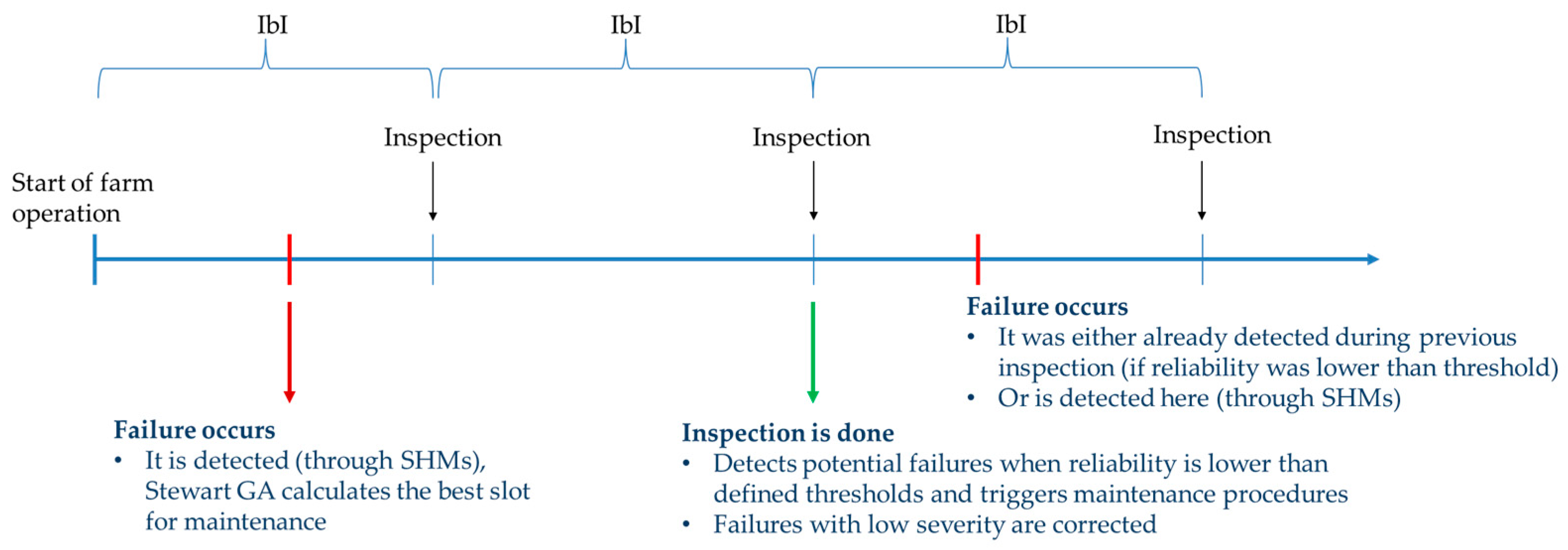
In practice, the model operates by evaluating the operational condition of each turbine over time, factoring in the interval between inspections (IbI) and the set inspection reliability thresholds from the “Captain GA”, alongside the failure predictions from the failure module. It systematically proposes and analyzes maintenance actions in response to each identified failure event. Turbines are presumed to be equipped with Structural Health Monitoring (SHM) systems that detect actual failures as they occur, an assumption that aligns with studies indicating SHM systems can allow for less frequent inspections without sacrificing revenue over the project’s lifespan [18]. However, SHM’s detection capabilities are considered, under the present research, to only detect already existing failures. In contrast, regular inspections aim to preempt potential failures by measuring a component’s reliability against established thresholds. If reliability is found to be below these thresholds during an inspection, a maintenance action is scheduled, which is aimed at fully restoring the component’s reliability. A depiction of an example for the timeline of a turbine under the developed model is proposed in Figure 5.
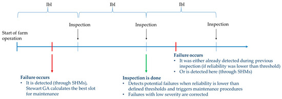
Figure 5.
Depiction of a maintenance timeline for floating offshore wind turbines under the present model, detailing scheduled inspections, real-time failure detections, and the resulting maintenance actions produced when a failure is detected or anticipated.
2.3. Failure Detection Module
The developed model integrates within a module designed to forecast component failures. Given the absence of real-world failure data for offshore wind farms, the module relies on failure rates and operational cost data derived from the research by James Carroll et al. [19], distributing failures stochastically over the entire duration of the analysis period considered for model simulation. Carroll et al. [19] attribute the severity of the failures of each subsystem based on the cost range of correcting a certain failure. The failure distribution output of the farm tested under the present research is obtained using a Monte Carlo simulation—a computational algorithm that relies on repeated random sampling to obtain numerical results, which in this case, predicts the timing of failures. The module operates under the assumption that failures follow an exponential distribution, which is a common hypothesis for failure analysis in the absence of more detailed data. The failure rates per component for minor repairs, major repairs, and replacements are presented below in Table 1.

Table 1.
Failure rates assumed for the failure detection module developed, collected from James Carroll et al. [19].
The module uses these rates to generate a structured dataset that describes the failure events’ timings. A partial example of a list of simulated failures obtained from the proposed module is provided below in Table 2.
Table 2.
Example of the partial output of the failure events as provided by the failure module. NA events are related to inspections (one per turbine).
Table 2 presents an hourly-based schedule of the main farm events, including type and severity of failures per turbine, as well as the inspection dates.
Given the stochastic nature of the exponential distribution, the reliability of the predictions from a single run of the model would be limited due to the inherent randomness of the process. To address this variability and enhance the robustness of the model’s forecasts, multiple instances of the model are run. Each iteration of the model uses a distinct sequence of failures based on the same underlying probability distributions, but with different random seeds, leading to varied outcomes. By aggregating the results from numerous simulations, the model averages out the randomness associated with individual runs. Consequently, the multiple runs collectively form a more comprehensive and accurate picture of the expected maintenance requirements over the analysis period, enabling more informed and strategic decision-making for maintenance scheduling.
2.4. Electricity Prices and Metocean Forecast Modules
Within the scope of this research, two distinct but interconnected modules have been integrated to process critical environmental data and energy market dynamics. The model assimilates historical electricity price data from 2017 to 2022 obtained from the OMIE database, which is the entity in charge of the Iberian energy market (MIBEL) [20]. These historical data are treated within the model as a predictive estimate, forecasting prices 30 days into the future to simulate a realistic decision-making environment. Such an approach ensures that maintenance scheduling will align with periods of maximum energy price to optimize revenue.
For metocean conditions, the model integrates wind and wave data acquired from the ERA5 reanalysis dataset, corresponding to the geographic coordinates nearest to the offshore wind farm. ERA5 provides access to a dataset of weather station data collected since 1950 to deliver hourly estimates of atmospheric, oceanic, and land climate variables over a global grid, with each cell spanning across 30 × 30 km [21]. For the purpose of this study, the following key parameters are used:
- Significant wave height, providing an average measure of the highest one-third of waves.
- The u component (eastward) and v component (northward) of the 10 m wind. These values have been adjusted to turbine height by extrapolating the wind speed from the standard 10 m height to 119 m, using the logarithmic wind profile equation, to reflect the actual hub height of the wind turbine considered.
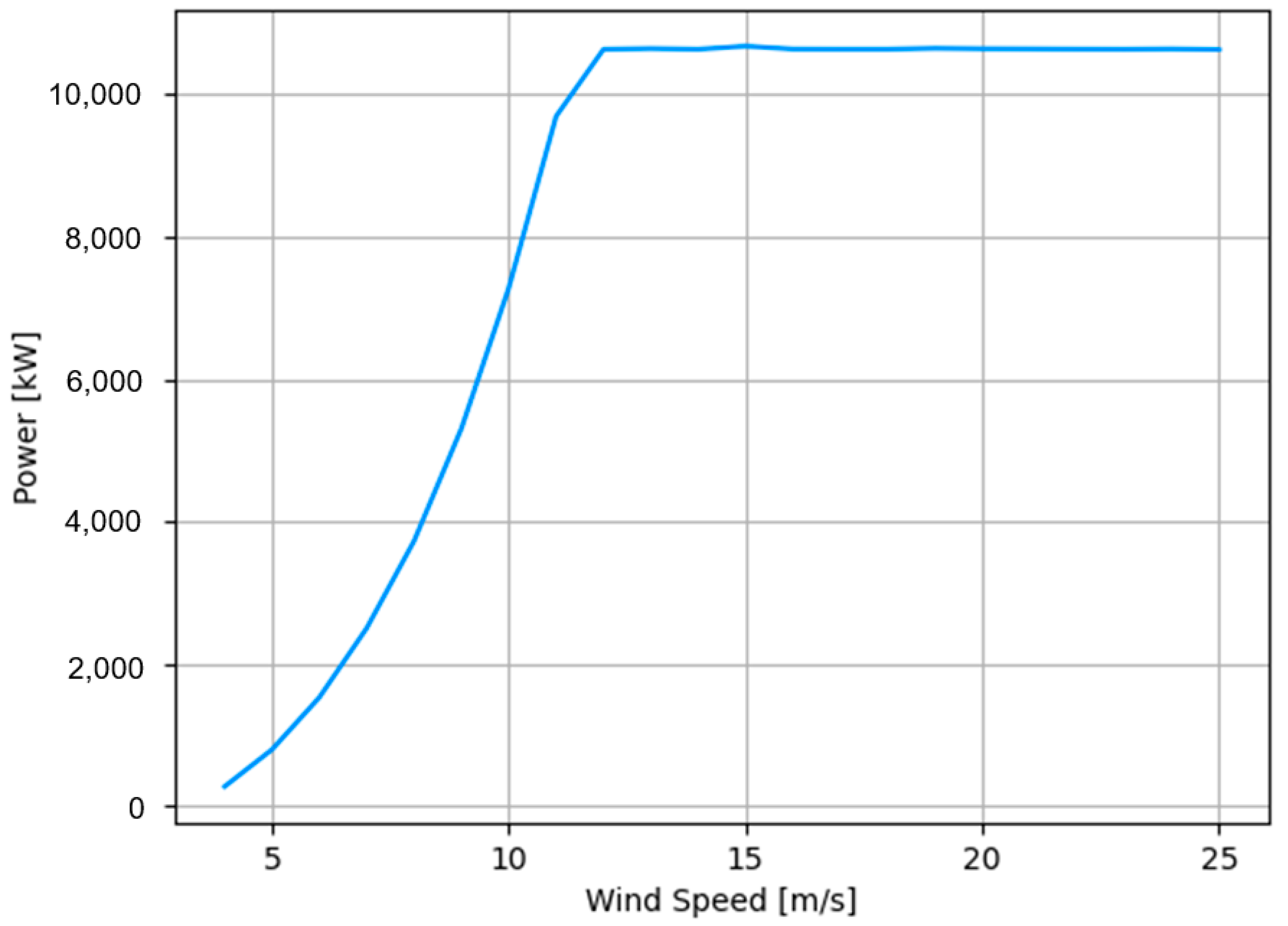
The absence of public data on the Vestas 8.3 MW turbine was overcome using the DTU 10 MW reference turbine [22,23]. This reference turbine serves as a scientific standard, allowing for the comparison of research outcomes between different research groups. By using the same turbine model, results can be consistently compared across different research. Employing the reference turbine’s power curve (see Figure 6) in conjunction with real-time electricity pricing and metocean data enables an accurate hourly forecast of energy production and associated revenue. This becomes a feedback mechanism for the model’s decision-making, informing the selection process of optimal maintenance timing to enhance the operational profitability of each turbine.

Figure 6.
Power curve of the 10 MW DTU reference turbine used within the present research [24].
The model also accounts for production halts during major repairs and anticipates downtime when spare parts are in transit. This allows for the preemptive shutdown of turbines to prevent compounding damage, a measure that safeguards other components and overall turbine integrity.
2.5. Cost and Logistic Assumptions
This section discusses and presents the cost and logistical assumptions assumed in this research for maintenance operations that require towing turbines to port (tow-to-port). The data draw on insights from Carroll et al. [19] work and on the internal databases of WavEC, reflecting the direct and indirect expenses associated with different maintenance activities—see Table 3.
Table 3.
Cost and logistic assumptions considered under the present research. Collected from James Carroll et al. [19] and WavEC internal database.
The maintenance costs for the key subsystems requiring tow-to-port procedures are classified into minor repairs, major repairs, and major replacements. Each category assumes distinct costs, reflecting the severity and complexity of the maintenance required. The expenditure associated with minor repairs is comparatively low, while major repairs and replacements incur significantly higher costs due to their comprehensive nature and the need for specialized equipment and labor. For the present research, it is assumed that TTP replacement events can be produced in just 72 h. Nonetheless, this value can be highly optimistic, particularly for newer farms or farms that do not have support ports in the vicinities. For example, recently, at the Kincardine OSW farm, which is floating and also counts on the Windfloat semi-submersible platform, total time for one TTP operation was of an astounding 94 days [25]. This operational experience highlights the need for optimizing O&M actions for floating OSW farms, as well as the need for adequate support infrastructure to accommodate the exigent needs of newer O&M strategies.
The logistic component of the model considers the type of vessel required for each maintenance activity—CTV (Crew Transfer Vessel), SOV (Service Operation Vessel), and DOCK (Docking Services). The choice of vessel is dictated by the specific maintenance operation, with DOCK being essential for major replacements (assuming the use of an SOV to execute the towing process). The associated costs are influenced by factors such as rental rates, human resources, and the duration of the maintenance procedure. The costs of renting vessels and the potential downtime must be factored into the overall budgeting and scheduling of maintenance operations. The research assumes at this stage that vessels are always available, although this may not reflect the real-world scenario and could introduce a level of uncertainty in the logistics planning. Table 4 presents the vessels required for each failure type and for each turbine part considered under this research.
Table 4.
Vessels required for each component, detailed by failure type.
The model accounts for hourly rates and daily costs for each vessel type. These rates include not only the base rental cost but also fuel charges and other operational expenses. For instance, the CTV has a lower hourly rate compared to the SOV and DOCK, but its operational costs per day might be less favorable when considering longer maintenance windows and conjoined maintenance operations. These values are presented in Table 5.
Table 5.
Costs of operating each vessel type.
The model also incorporates maximum operational wind speeds and wave heights for each vessel type, which are essential for ensuring safety and feasibility of maintenance operations. These thresholds are aligned with the industry practices and were retrieved from WavEC’s database. If metocean conditions exceed these thresholds, maintenance activities will be delayed, which will consequently impact the overall scheduling and costs—see Table 6.
Table 6.
Maximum operational metocean conditions for maintenance operations.
Lastly, the availability of spare parts in the warehouse and the lead time for ordering components from manufacturers are crucial parameters for the model (in fact, the availability of each part in the warehouse is one of the genes assumed for the “Stewart GA”). These factors influence maintenance scheduling, as the lack of immediate part availability could lead to extended downtimes, especially in the event of unscheduled maintenance requirements. The integration of these cost and logistic assumptions provides realistic estimates of the direct costs associated with specific maintenance activities.
2.6. Genetic Algorithm Parameters/Simulation Parameters
In this research, two distinct sets of parameters, which frame the evolutionary search process within each algorithm’s loop, were defined for the “Captain GA” and the “Stewart GA”. These are summarized below in Table 7.
Table 7.
Genetic algorithms’ parameters for the developed model.
The parameter “Number of Averages” is unique to the “Captain GA”, reflecting the emphasis of the developed model on long-term strategic decision-making by averaging results over multiple simulations to address the stochastic nature of the failure generation model.
The chromosomes of both genetic loops present the blueprints of the algorithms, being formed by the decision variables essential to maintenance scheduling and decision-making. The “Captain GA” chromosome is constituted by parameters that influence long-term strategic decisions, including the interval between inspections (IbI) and repair thresholds for various components, where each gene corresponds to a vital decision variable for long-term planning. Specifically, this chromosome can be represented as:
where the IbI ranges from 1 to 12 months, and the repair thresholds for each of the = 5 turbine parts considered may vary from 10 to 90%. The “Stewart GA” chromosome encodes operational decisions such as the optimal maintenance hour within a short-term horizon and the availability of spare parts in the warehouse. It can be represented as:
where the optimal maintenance hourly slot can take a value between zero and 720 (7 days), and the spare part availability is a binary variable, which may take a value of zero (no spare part available) or one. These structures allow the algorithms to efficiently seek optimal maintenance parameters that maximize the short-term and long-term profitability of the farm.
2.7. Use of Large Language Models
In the preparation of this manuscript, the Large Language Model (LLM) ChatGPT provided by OpenAI was employed specifically for the improvement and revision of the written text. Adhering to the Research and Publication Ethics set forth by MDPI [26], the utilization of ChatGPT was confined strictly to the enhancement of narrative clarity, coherence, and grammatical accuracy within the manuscript. The authors clarify that ChatGPT was not used in any other stage of the research process, including but not limited to the conceptualization, methodology development, or the implementation of the Python code underlying the model’s architecture.
3. Results
This section details the outcomes derived from the application of the GAs for optimizing maintenance scheduling and strategic decision-making for floating offshore wind farms. The results shown here demonstrate the model’s capacity to provide actionable insights under the assumptions and constraints previously outlined.
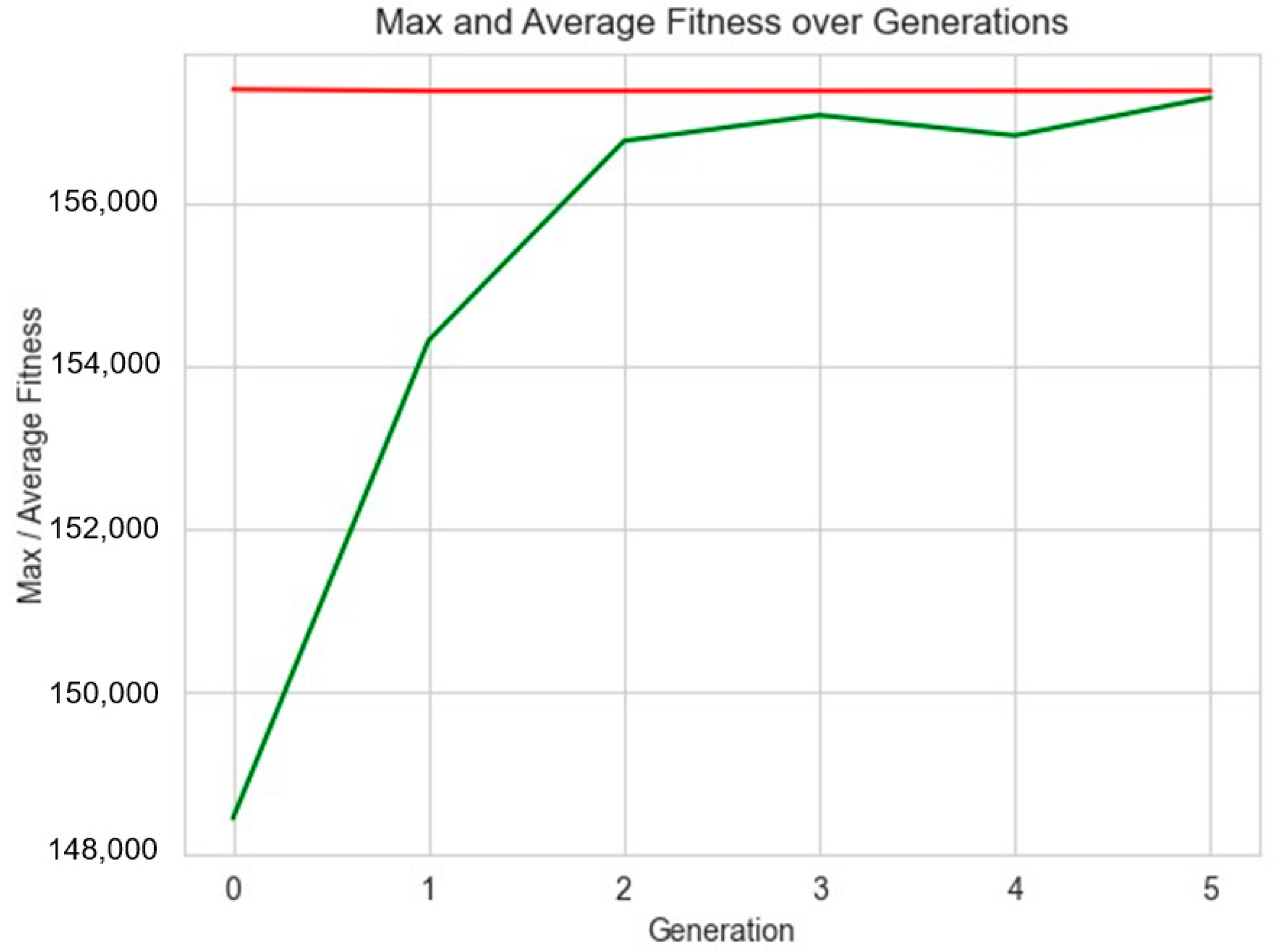
3.1. Stewart GA Convergence
The “Stewart GA” exhibits rapid convergence, typically achieving near-optimal solutions within just a few generations. This quick convergence, as illustrated in Figure 7, showcases the algorithm’s effectiveness in finding efficient solutions within time constraints. The graph presents both the average and maximum fitness across generations, illustrating a steep ascent of the average fitness towards highest levels of fitness within the initial few generations, followed by stabilization. Although the results for five generations are shown here, the number of generations used for the final simulations was two, according to what is established in Table 7.

Figure 7.
Convergence curve for the Stewart GA. Green—average fitness over generations; red—maximum average over generations.
Table 8 presents an example of a detailed breakdown of the optimal maintenance schedules proposed by the “Stewart GA” for one specific failure, which are highly dependent on weather conditions, electricity prices, and parts availability, as explained earlier.
Table 8.
Example of the outputs obtained from the Stewart GA, showing the dates of detection of failures and the respective best dates for maintenance in function of the balance of the 30-day period analyzed.
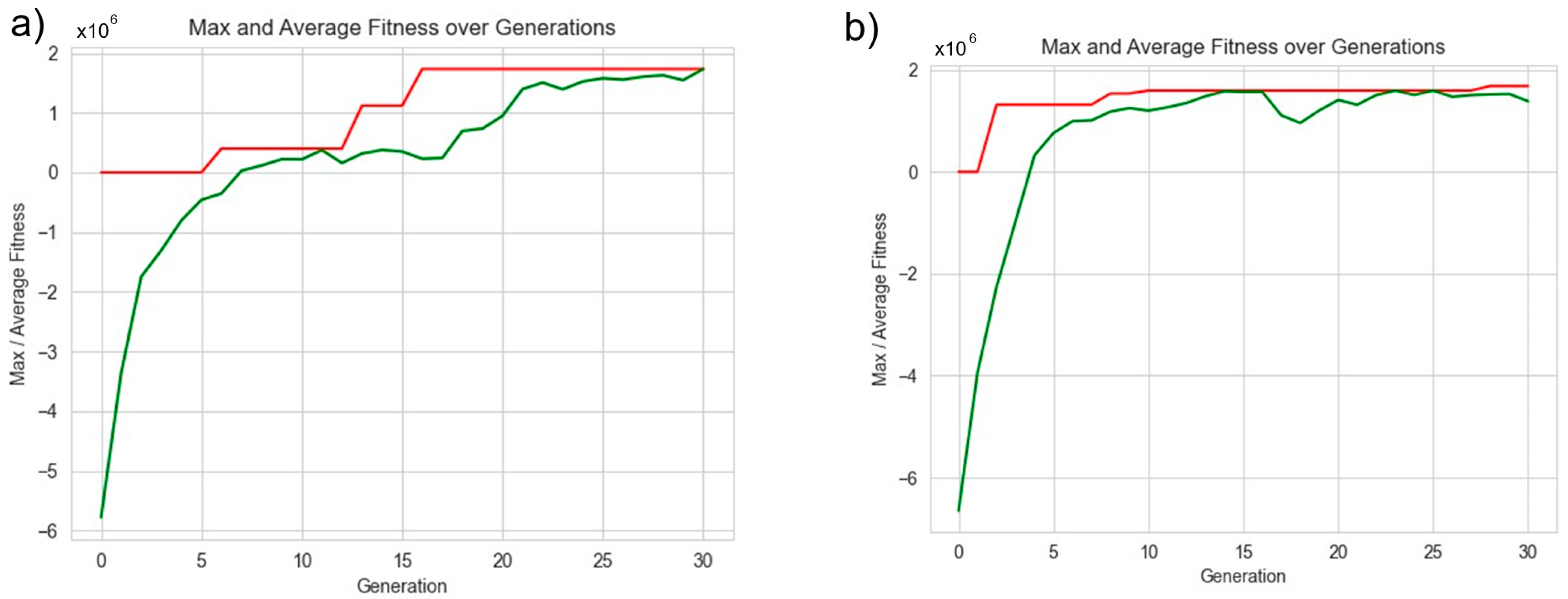
3.2. Captain GA Convergence
In contrast to the “Stewart GA”, the “Captain GA” tackles more complex, long-term strategic decisions, which is reflected in its slower convergence rates shown in Figure 8. This model requires averaging multiple simulations to mitigate result variability due to the stochastic nature of the failure module. The convergence curves from two separate runs presented in Figure 8 reveal the importance of maintaining genetic diversity to avoid local optima and ensure robust solutions over longer time spans.
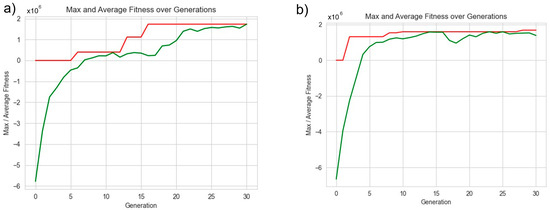
Figure 8.
Two convergence curves for two independent runs of the Captain GA (a,b). Green—average fitness over generations; red—maximum average over generations.
To elucidate the practical application of the “Captain GA”, Table 9 presents an example of the output generated for strategic decision-making under the current case-study. The table presents the optimal genes (strategies) identified for the best solution, alongside the predicted financial impacts over a five-year operational period of the wind farm for the best four solutions.
Table 9.
Example of the output obtained from the “Captain GA” showing the best genes calculated for each run and the respective best balances over a period of 5 years of operation of the farm.
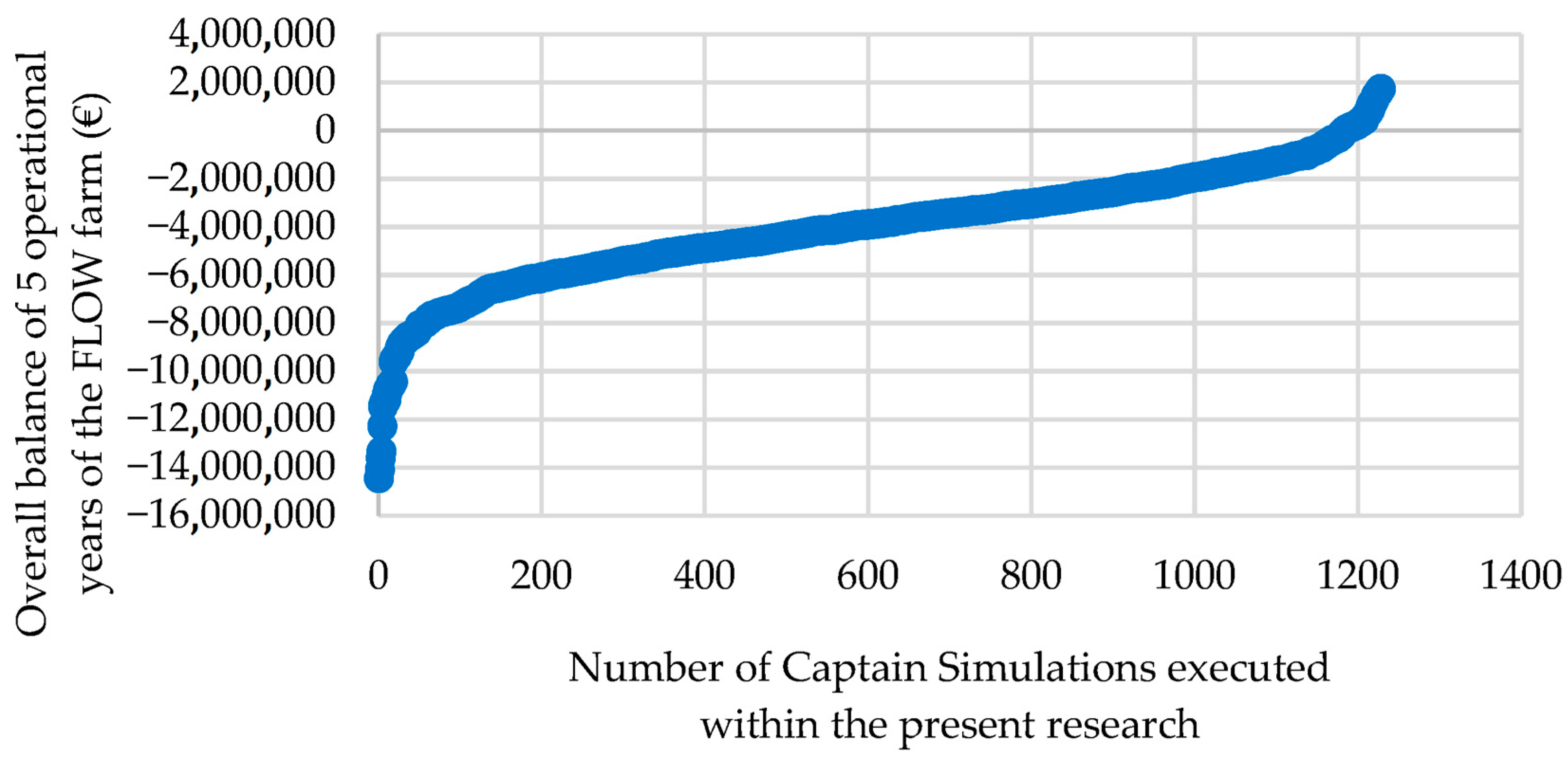
Figure 9 presents the cumulative balance from all simulations conducted using the “Captain GA”—the aggregated performance across multiple runs rather than a time-sequential progression of the algorithm. The stages observed for this specific genetic algorithm’s optimization process are described next:
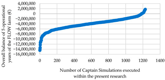
Figure 9.
Cumulative curve of all Captain simulations run in function of the total balance of the farm operating for 5 years.
Early Convergence: The GA rapidly identifies promising solutions early in the evolutionary process, leading to a steep initial increase in the curve. This phase represents substantial improvements over random initial conditions.
Plateau Phase: Following the sharp initial gains, the rate of improvement slows significantly. During this phase, the GA incrementally refines the solutions. The plateau indicates a period where the algorithm converges towards a local maximum and struggles to find new, significantly better solutions without additional algorithmic interventions such as increased mutation rates or crossover events.
Final Divergence: Contrary to what might be expected in a typical GA progression—where a late convergence might suggest finding a global optimum—the observed divergence is indicative of the stochastic elements of the simulation. This divergence emphasizes the impact of random events on the solutions’ effectiveness and the challenge in achieving consistently higher fitnesses—it might also point out that consistent global optima were not found for the total number of simulations run.
3.3. Long-Term Strategic Insights
The “Captain GA” results were analyzed using single and multiple linear regression models (MLRMs) to evaluate the significance of various operational variables on the farm’s financial balance over a five-year operation period. The single linear regression models were computed between the balance (the dependent variable) and the genes of the best solutions (the independent variables). However, for these single linear regression models, little correlation was found—this was expected as the model is influenced by several variables rather than just one. For this reason, a multiple linear regression model was built. The results of this MLRM analysis are summarized in Table 10, which presents the regression statistics and coefficients for each variable considered.
Table 10.
Results for the multiple linear regression model for the cumulative balance results of all simulations run for the “Captain GA”.
Based on the regression analysis, all thresholds demonstrate significant impact on the financial balance of the farm. Specifically, Thre4 was subjected to a cubic root transformation. This transformation addresses non-linear relationships within the data, rendering the variable Thre4 more adequate for modeling and, for this specific purpose, statistically significant.
The results for the IbI (interval between inspections) coefficient suggest that longer intervals between inspections correlate positively with higher financial returns. This could be attributed to decreased scheduled operational stoppages and lower inspection costs over the evaluation period.
Notably, Thre 1, Thre 5, and Thre 6 exhibit negative coefficients, suggesting that lower repair thresholds are advantageous for the pitch/hydraulic system, support structures, and transformer, respectively. This indicates that less frequent inspections could be beneficial, potentially reducing unnecessary maintenance activities and costs. For the support structures (tower and foundation), this can be explained as they are designed to last the duration of the project without replacement. On the other hand, the transformer and pitch/hydraulics subsystems possess very low major failure rates that require replacement (according to Table 3).
Finally, Thre 2 (generator), Thre 3 (gearbox), and Thre 4 (blades) show positive coefficients, emphasizing the need for active inspection and diligent maintenance of these components to ensure optimal operational availability and profitability.
3.4. Short-Term Tactical Insights
3.4.1. Logistic Regression Model for Spare Parts
Understanding the operational impact of maintaining a stock of spare parts compared to ordering replacements upon failure is critical in operational management. This section examines the benefits of proactive inventory management using a logistic regression model, with electricity price as a predictor of the needs for spare parts during equipment failure incidents. The model’s fitting to the data was confirmed to be statistically robust, offering several noteworthy points (see results in Table 11).
Table 11.
Logistic regression model statistics.
The model’s performance, indicated by the log-likelihood of −1135.7, reflects a satisfactory fit, notably when juxtaposed with the LL-Null value of −1198.4. Such a distinction highlights the predictive capability introduced by incorporating the electricity price into the model. The likelihood ratio test, manifested in an LLR p-value of approximately 4.19 × 10⁻²⁹, robustly establishes the statistical significance of the model, suggesting a substantial improvement over a model devoid of predictor variables. The pseudo-R2 value, at 0.05232, is relatively modest, which is not uncommon in logistic regression models given their nature. This metric reflects the proportion of variability in the dependent variable that is explained by the model. The low value suggests that while electricity pricing does have an influence, the decision-making process regarding spare parts inventory is multifaceted and likely influenced by numerous factors. It is essential to recognize that this model is multivariate, and its outcomes are partly shaped by the stochastic nature of the failure module generator.
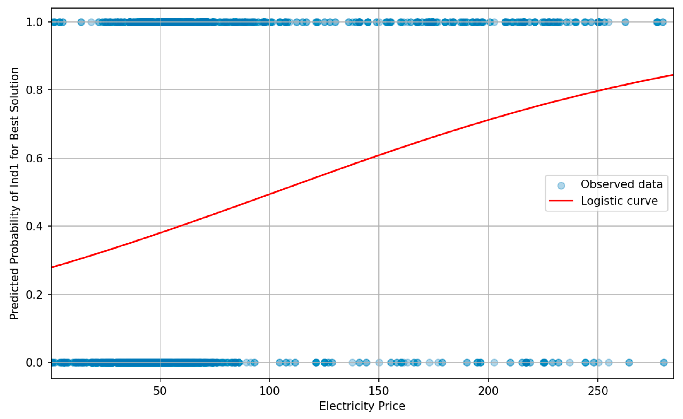
This significant association between electricity prices and operational choices related to spare parts inventory management corroborates the hypothesis that higher electricity prices can tip the scales in favor of having a well-stocked inventory. Figure 10 presents the regression curve for the obtained logistic regression model.

Figure 10.
Logistic regression curve for the possibility of having the part stored in a warehouse in comparison to ordering it after a failure is detected.
The logistic regression model demonstrates that higher electricity prices moderately increase the likelihood of being preferable to having the part to be replaced stored inhouse. However, the dataset is more robust at lower electricity prices, leading to more confident model predictions in this range. As the price increases, the sparser data result in less precise estimates.
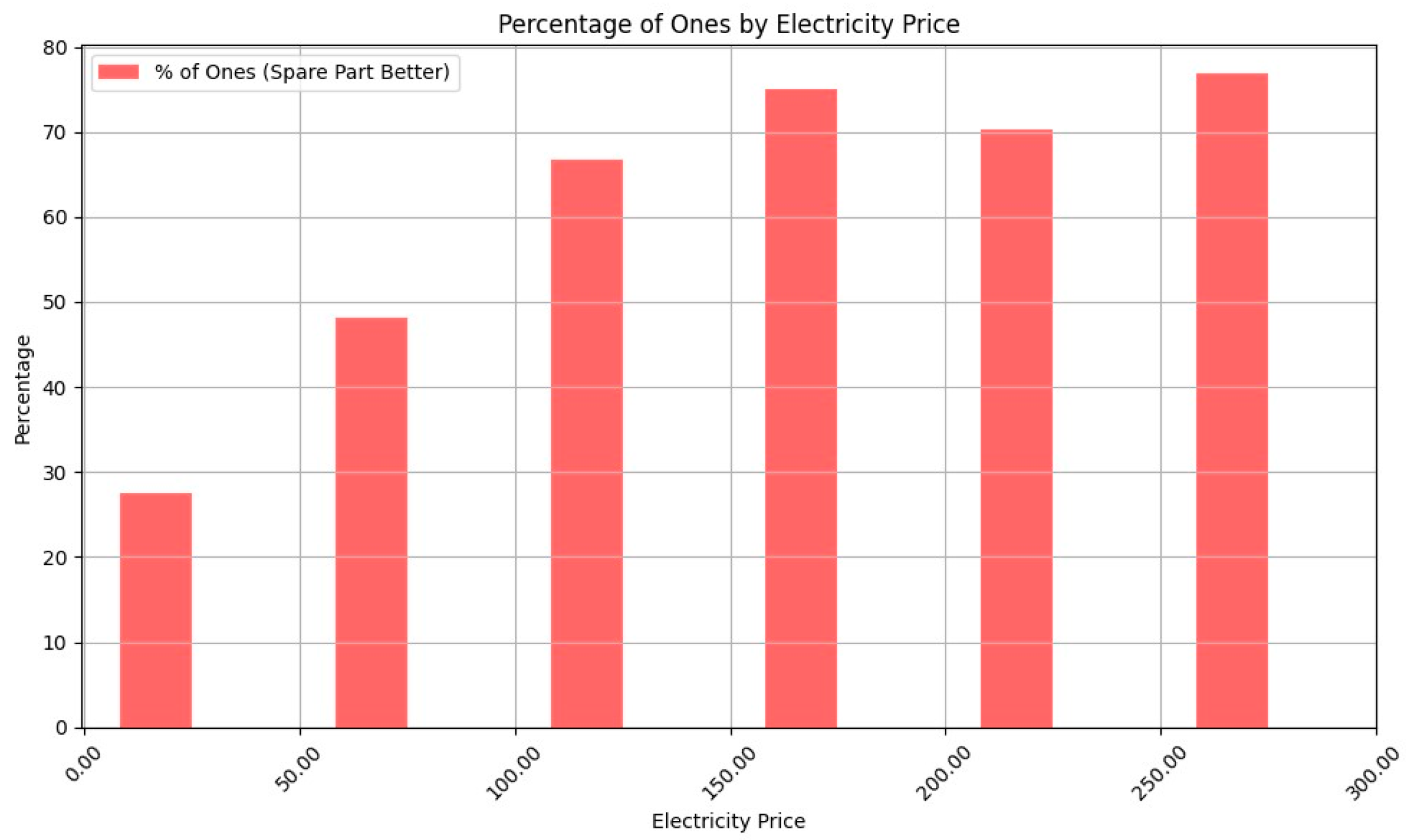
Figure 10 and Figure 11 show that as electricity prices increase, the benefits of having parts stored inhouse increase. The logistic regression indicates that for electricity prices above EUR 150/MWh, there is a fifty percent chance that it will be better to have spare parts stored for all five failure types that may require replacement. Figure 11 shows that when the electricity price is above EUR 100/MWh, the percentage of registered results with ones (part available in warehouse) is consistently above 50%.

Figure 11.
Percentage of ones varying with the electricity price.
3.4.2. Influence of Weather Conditions on Maintenance Scheduling
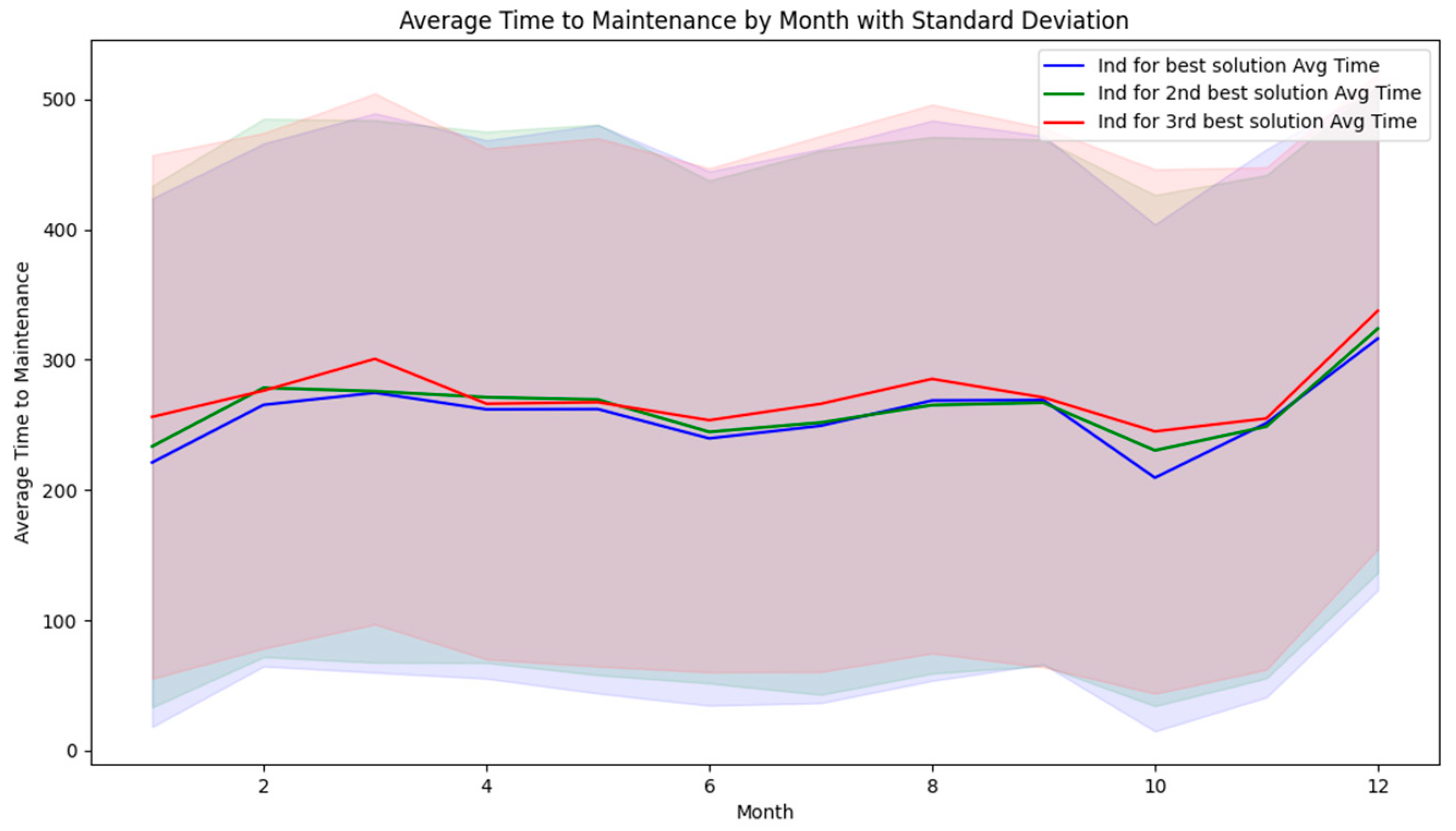
Figure 12 illustrates the trend of average best slots for time to maintenance across the months of the year, along with the associated standard deviations. This depiction allows for observation of not only the average preferred timing for maintenance but also the variability inherent in these decisions.
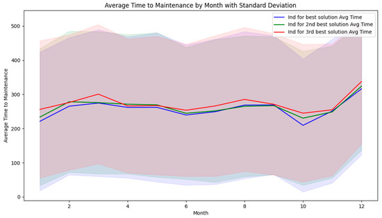
Figure 12.
Trend of average best slots for time to maintenance varying with each month of the year and the respective standard deviations on the background areas.
The trend suggests that certain months may more readily offer conditions for maintenance activities than others, a fact that should be factored into the strategic planning of operations. Furthermore, the standard deviations reflect the range of variability within each month, providing insight into the potential risk of deviating from the average (which, nonetheless, do not vary much from month to month).
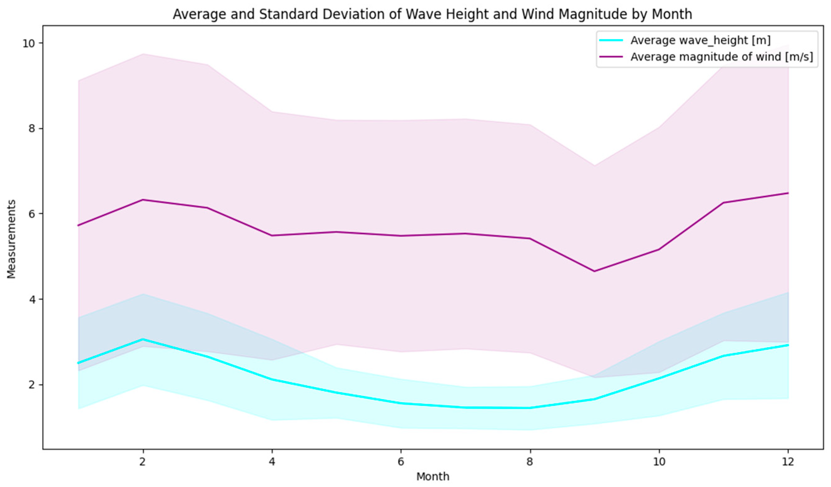
Figure 13 complements this discussion by plotting the fluctuations in average wind speeds and significant wave heights, again broken down by month and superimposed with their corresponding standard deviations.
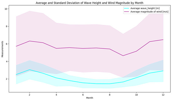
Figure 13.
Trend of averages (lines) and respective standard deviations (background areas) of wind speed and significant wave height for the 12 months of the year for the 5-year period analyzed here.
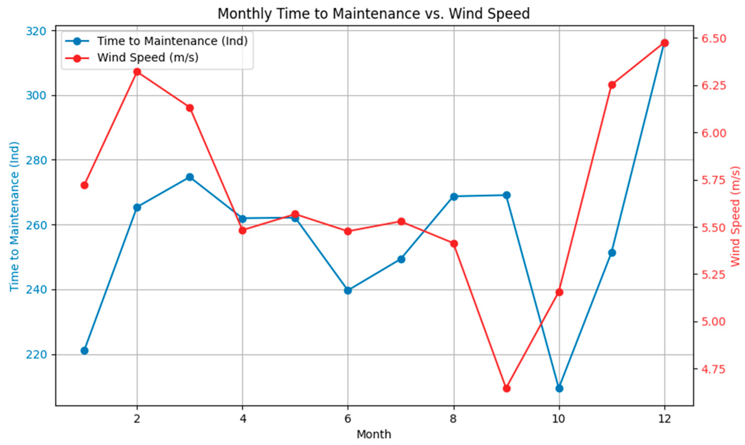
A visual correlation between Figure 12 and Figure 13 is readily apparent. As one might intuitively expect, the windows for optimal maintenance times are influenced by weather patterns. This relationship is teased out in more detail in Figure 14, which concurrently shows the wind speeds and the timing of maintenance activities across the months of the year.
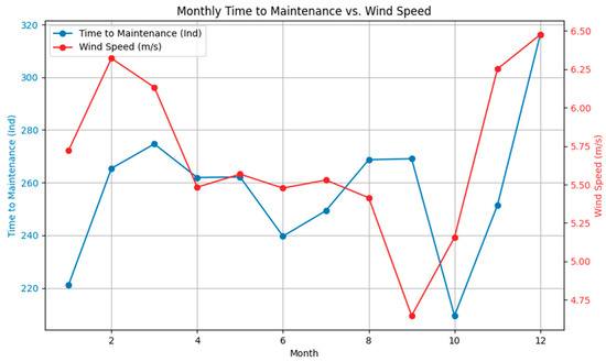
Figure 14.
Evolution of wind speed and time to maintenance with the months, suggesting a moderate correlation between both.
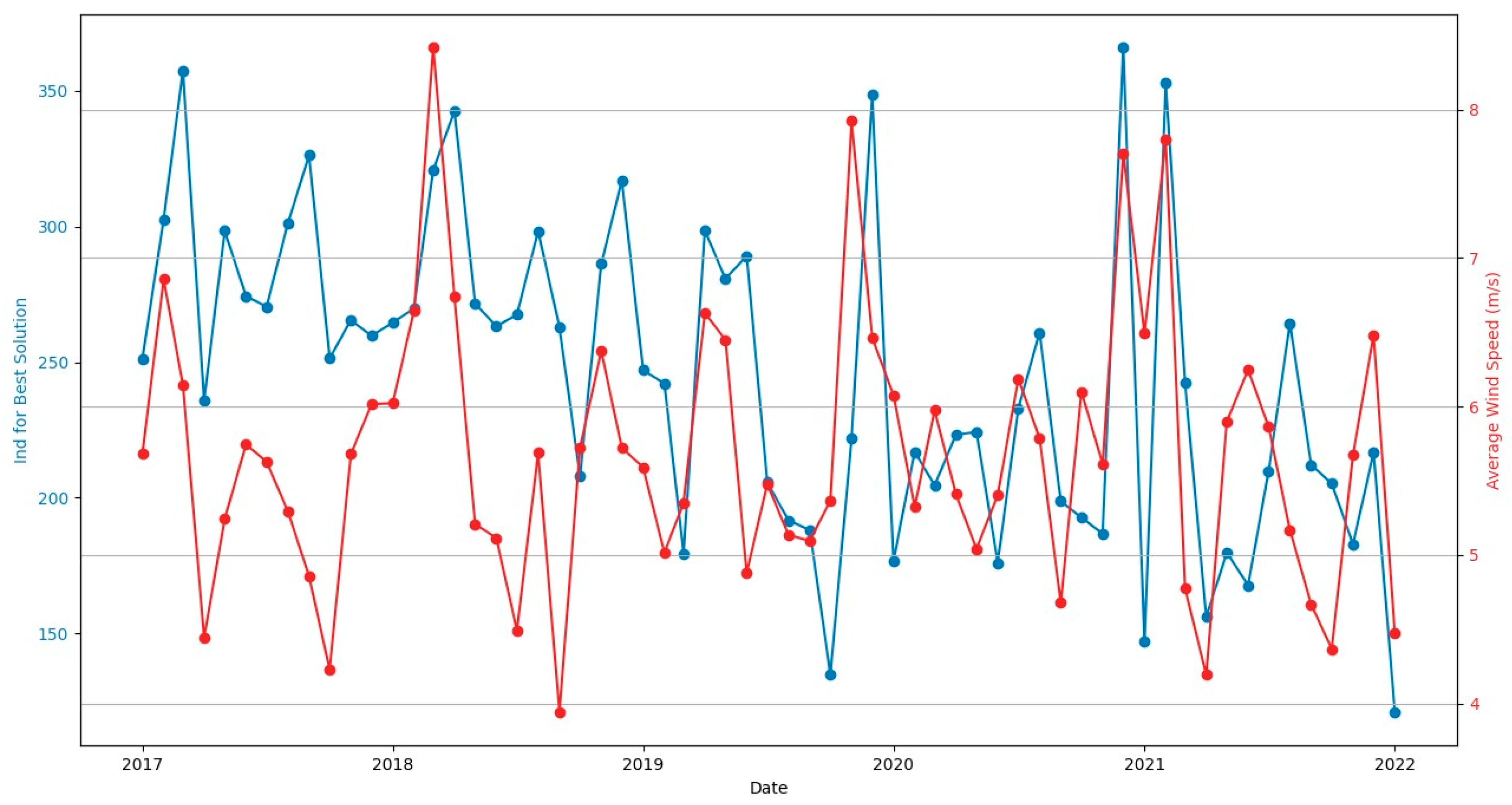
To further probe this relationship, Figure 15 plots the trends of wind speed against maintenance times over a five-year span. While a simple Pearson correlation might not yield significant results due to non-linearity and non-normal distribution of data, a Spearman correlation assesses the rank order between two variables, making it more robust against outliers and suitable for non-parametric data, providing a clearer understanding of how these two factors (wind speed and time to maintenance) relate [27].

Figure 15.
Trend of average wind speed and best slot for maintenance for the 5-year period analyzed in this research.
The application of Spearman’s rank correlation coefficient to the study’s data presents insights on the interaction between wind speed and maintenance scheduling. With a coefficient of 0.31, the analysis suggests a positive though modest relationship; as wind speeds escalate, so might the intervals to scheduled maintenance. This correlation, while not robust, is still telling. The moderate nature of this correlation indicates that while wind speed is a factor, it is not the sole determinant of maintenance schedules.
In practical terms, the weak to moderate correlation still holds operational significance. For instance, in planning and scheduling, acknowledging that higher wind speeds can be associated with extended periods to maintenance allows for more nuanced planning. This might include allocating additional resources or adjusting timelines to accommodate the increased likelihood of maintenance delays.
The correlation between significant wave height and best time for maintenance was also evaluated, with no relevant interactions detected between the two, which is surprising. This could be due to the maximum operational metocean conditions for maintenance operations defined in Table 6. If the available vessels for maintenance operations would sustain lower wave conditions than those assumed for this research, the significance of the wave weight on the definition of the best time for maintenance could possibly increase.
To further understand if the wind speed could be used to predict the time to maintenance, the Granger causality test was implemented as part of the current analysis. This statistical method is particularly suited for time-series data where past values of one variable might contain information that could predict future values of another [28].
At lag 1, with a p-value hovering just below 0.05, there is a tentative indication that wind speed could have a bearing on the projection of maintenance times. This initial lag provides insights into the potential predictive capacity of wind speed, although with limited confidence. When the analysis extends to lags 2 through 4, the p-values drop significantly, reinforcing the premise that wind speed has a meaningful influence on predicting maintenance scheduling. The strength of this relationship intensifies with the consideration of more historical data points.
It is worth noting that the Granger causality test does not imply a direct cause-and-effect mechanism, but suggests that knowledge of past wind speed values can be statistically useful in forecasting maintenance timings. This finding is valuable for operational strategies that seek to optimize maintenance planning based on weather trends.
4. Conclusions
The study conducted in this paper focused on the development of a model to support decision-making on the operational management of floating offshore wind (FOW) farms, utilizing nested genetic algorithms for the decision-making process involved in maintenance. Emphasis was placed on the unique maintenance strategies required by the complex dynamics of deep waters (notably tow-to-port), where traditional fixed-bottom turbines are not viable.
For short-term tactical decisions, the study’s outcomes suggest that the timing of maintenance operations is firstly influenced by wind conditions. In addition, a logistic regression model determined that increased electricity prices might justify the presence of spare parts on-site, offering a potential reduction in operational disruptions. Spearman correlation analysis and the Granger causality test further support the relationship between wind speed and maintenance scheduling, emphasizing the value of historical weather data in anticipating maintenance needs.
In terms of long-term strategic considerations, the multiple linear regression model analyzed the farm’s financial balance over five years. It was found that specific operational factors like inspection intervals have a significant impact on the farm’s financial health: higher IbIs lead to improved operational profitability. The model also suggests that thoroughly inspecting generators, gearboxes, and blades can improve the profitability of the farm, while pitch/hydraulic, support structures, and transformers do not benefit from exhaustive inspections of their condition. These insights could guide resource allocation and prioritize maintenance efforts that contribute most significantly to the operational efficiency and economic viability of wind farms.
Additionally, this study’s relevance extends to the economic implications of maintenance strategies under varying market conditions. While the Windfloat Atlantic, the case study referenced in this research, operates under a fixed feed-in tariff system, where electricity prices are fixed, future offshore wind farms are likely to encounter different economic frameworks for revenue. It is anticipated that many will operate under Contracts for Difference or may even need to compete directly within the existing electricity markets. This shift would make the findings on the correlation between electricity prices and the feasibility of having spare parts on-site increasingly pertinent. As the dynamics of electricity pricing evolve, the insights gathered from this research could become crucial for optimizing maintenance strategies and managing operational costs in a competitive market landscape.
This paper aimed to demonstrate the application of complex genetic algorithms in supporting both immediate and future-oriented maintenance strategies for floating offshore wind operations. While the conclusions drawn have a more academic tilt, the model holds promise for practical adaptation, allowing integration with actual operational data to support real-time decisions in diverse farm conditions.
Author Contributions
Conceptualization, D.D. and M.V.; methodology, D.D. and M.V.; software, M.V.; validation, D.D. and M.V.; formal analysis, D.D. and M.V.; investigation, D.D. and M.V.; resources, D.D. and M.V.; data curation, D.D. and M.V.; writing—original draft preparation, D.D. and M.V.; writing—review and editing, D.D. and M.V.; visualization, M.V.; supervision, D.D.; project administration, D.D. and M.V.; funding acquisition, D.D. and M.V. All authors have read and agreed to the published version of the manuscript.
Funding
This research was funded by the UT Austin in Portugal Program under the Short-Term Research Internships—Year 2022.
Institutional Review Board Statement
Not applicable.
Informed Consent Statement
Not applicable.
Data Availability Statement
The authors may consider making the Python code developed for this study available upon request. Interested parties should contact the corresponding author to discuss access.
Acknowledgments
The authors acknowledge the use of OpenAI’s Large Language Model, ChatGPT, in the manuscript preparation for enhancing the narrative clarity, coherence, and grammatical accuracy. This adherence ensures compliance with the Research and Publication Ethics outlined by MDPI.
Conflicts of Interest
The authors declare no conflicts of interest.
References
- Jansen, M.; Staffell, I.; Kitzing, L.; Quoilin, S.; Wiggelinkhuizen, E.; Bulder, B.; Riepin, I.; Müsgens, F. Offshore wind competitiveness in mature markets without subsidy. Nat. Energy 2020, 5, 614–622. [Google Scholar] [CrossRef]
- GWEC. GWEC Global Wind Report 2022; Global Wind Energy Council: Bonn, Germany, 2022; p. 75. [Google Scholar]
- GWEC. Floating Offshore Wind—A Global Opportunity; Global Wind Energy Council: Bonn, Germany, 2022. [Google Scholar]
- Vieira, M.; Henriques, E.; Amaral, M.; Arantes-Oliveira, N.; Reis, L. Path discussion for offshore wind in Portugal up to 2030. Mar. Policy 2019, 100, 122–131. [Google Scholar] [CrossRef]
- Portugal Energia. Plano Nacional Energia E Clima (PNEC) 2021–2030. Available online: https://www.portugalenergia.pt/setor-energetico/bloco-3/ (accessed on 11 January 2022).
- House, T.W. FACT SHEET: Biden-Harris Administration Continues to Advance American Offshore Wind Opportunities. Available online: https://www.whitehouse.gov/briefing-room/statements-releases/2023/03/29/fact-sheet-biden-harris-administration-continues-to-advance-american-offshore-wind-opportunities/ (accessed on 8 February 2024).
- Renews Ltd. Tow-To-Port O & M Strategy “May Hold Back Floating Wind”. Available online: https://renews.biz/83732/tow-to-port-may-hold-back-floating-wind-projects/ (accessed on 10 February 2024).
- Bayati, I.; Efthimiou, L. Onsite Major Component Replacement Technologies for Floating Offshore Wind: The Status of the Industry; WFO—World Forum Offshore Wind: Singapore, 2023. [Google Scholar]
- McMorland, J.; Collu, M.; McMillan, D.; Carroll, J. Operation and maintenance for floating wind turbines: A review. Renew. Sustain. Energy Rev. 2022, 163, 112499. [Google Scholar] [CrossRef]
- Zhao, C.; Liu, H.; Qu, X.; Liu, M.; Tang, R.; Xie, A. Reliability analysis of floating offshore wind turbine generator based on failure prediction and preventive maintenance. Ocean Eng. 2023, 288, 116089. [Google Scholar] [CrossRef]
- De Matos Sá, M.; Correia Da Fonseca, F.X.; Amaral, L.; Castro, R. Optimising O & M scheduling in offshore wind farms considering weather forecast uncertainty and wake losses. Ocean Eng. 2024, 301, 117518. [Google Scholar] [CrossRef]
- Rinaldi, G.; Thies, P.R.; Johanning, L. Current Status and Future Trends in the Operation and Maintenance of Offshore Wind Turbines: A Review. Energies 2021, 14, 2484. [Google Scholar] [CrossRef]
- Correia da Fonseca, F.X.; Amaral, L.; Chainho, P. A Decision Support Tool for Long-Term Planning of Marine Operations in Ocean Energy Projects. J. Mar. Sci. Eng. 2021, 9, 810. [Google Scholar] [CrossRef]
- Wang, K.; Djurdjanovic, D. Joint Optimization of Preventive Maintenance and Spare Parts Logistics for Multi-echelon Geographically Dispersed Systems. In Asset Intelligence through Integration and Interoperability and Contemporary Vibration Engineering Technologies; Mathew, J., Lim, C.W., Ma, L., Sands, D., Cholette, M.E., Borghesani, P., Eds.; Lecture Notes in Mechanical Engineering; Springer: Cham, Switzerland, 2019; pp. 643–653. ISBN 978-3-319-95710-4. [Google Scholar]
- Li, M.; Jiang, X.; Carroll, J.; Negenborn, R.R. A multi-objective maintenance strategy optimization framework for offshore wind farms considering uncertainty. Appl. Energy 2022, 321, 119284. [Google Scholar] [CrossRef]
- Rinaldi, G.; Pillai, A.C.; Thies, P.R.; Johanning, L. Multi-objective optimization of the operation and maintenance assets of an offshore wind farm using genetic algorithms. Wind Eng. 2020, 44, 390–409. [Google Scholar] [CrossRef]
- Algorithms—DEAP 1.4.1 Documentation. Available online: https://deap.readthedocs.io/en/master/api/algo.html (accessed on 24 March 2024).
- Vieira, M.; Henriques, E.; Snyder, B.; Reis, L. Insights on the impact of structural health monitoring systems on the operation and maintenance of offshore wind support structures. Struct. Saf. 2022, 94, 102154. [Google Scholar] [CrossRef]
- Carroll, J.; McDonald, A.; McMillan, D. Failure rate, repair time and unscheduled O & M cost analysis of offshore wind turbines: Reliability and maintenance of offshore wind turbines. Wind Energy 2016, 19, 1107–1119. [Google Scholar] [CrossRef]
- Acesso aos arquivos|OMIE. Available online: https://www.omie.es/pt/file-access-list (accessed on 30 March 2024).
- Hersbach, H.; Bell, B.; Berrisford, P.; Hirahara, S.; Horányi, A.; Muñoz-Sabater, J.; Nicolas, J.; Peubey, C.; Radu, R.; Schepers, D.; et al. The ERA5 global reanalysis. Q. J. R. Meteorol. Soc. 2020, 146, 1999–2049. [Google Scholar] [CrossRef]
- Bak, C.; Zahle, F.; Bitsche, R.; Kim, T.; Yde, A.; Henriksen, L.C.; Hansen, M.H.; Blasques, J.P.A.A.; Gaunaa, M.; Natarajan, A. The DTU 10-MW Reference Wind Turbine. In Proceedings of the Danish Wind Power Research 2013, Fredericia, Denmark, 27–28 May 2013; p. 22. [Google Scholar]
- DTU 10-MW Reference Wind Turbine. Available online: https://www.hawc2.dk/models/dtu-10-mw (accessed on 30 March 2024).
- DTU_10MW_178_RWT_v1—NREL/Turbine-Models Power Curve Archive 0 Documentation. Available online: https://nrel.github.io/turbine-models/DTU_10MW_178_RWT_v1.html (accessed on 31 March 2024).
- Key Lessons in Floating Wind O & M. Available online: https://www.spinergie.com/blog/lessons-learned-from-heavy-maintenance-at-the-worlds-first-commercial-floating-wind-farm (accessed on 31 March 2024).
- MDPI Research and Publication Ethics. Available online: https://www.mdpi.com/ethics (accessed on 25 March 2024).
- Dodge, Y. Spearman Rank Correlation Coefficient. In The Concise Encyclopedia of Statistics; Springer: New York, NY, USA, 2008; pp. 502–505. ISBN 978-0-387-31742-7. [Google Scholar]
- Kirchgässner, G.; Wolters, J.; Hassler, U. Granger Causality. In Introduction to Modern Time Series Analysis; Springer Texts in Business and Economics; Springer: Berlin/Heidelberg, Germany, 2013; pp. 95–125. ISBN 978-3-642-33435-1. [Google Scholar]

Disclaimer/Publisher’s Note: The statements, opinions and data contained in all publications are solely those of the individual author(s) and contributor(s) and not of MDPI and/or the editor(s). MDPI and/or the editor(s) disclaim responsibility for any injury to people or property resulting from any ideas, methods, instructions or products referred to in the content. |
© 2024 by the authors. Licensee MDPI, Basel, Switzerland. This article is an open access article distributed under the terms and conditions of the Creative Commons Attribution (CC BY) license (https://creativecommons.org/licenses/by/4.0/).