Population Balance Modeling of Milling Processes: Are We Falsifying Breakage Kinetics and Distribution via Back-Calculation Methods?

Abstract

Population balance models (PBMs) for milling processes are based on two fundamental concepts: specific breakage rate function and breakage distribution function, which vary with particle size as well as design–operation conditions. The solution of the inverse problem, i.e., the estimation of these two functions’ parameters, may cause falsified kinetics and breakage distribution mechanisms. This perspective article aims to expose and mitigate various aspects of potential falsification, thus enabling the development of a robust PBM. Through an in-depth analysis of historical approaches to the PBM inverse problem and experimental observations, as well as the author’s recent contributions to the inverse methodology within the context of back-calculation methods, six principles have been offered: (i) include the governing physical phenomena and reduce errors in model building; (ii) reduce the number of model parameters via size–operation-dependent functional forms, hybrid approaches for back-calculation, and combination with CFD–DEM and other mechanistic models; (iii) generate a dense particle size distribution data set obtained at various milling times and/or locations; (iv) ensure a grid-independent solution with a sufficient number of size classes; (v) use a global optimization-based back-calculation method for parameter estimation and provide standard errors of the estimates; and (vi) test the predictive capability of the PBM. This perspective article boosts awareness of various challenges involved in the solution of the inverse PBM problem as pertinent to milling processes and provides researchers with six principles to minimize falsified kinetics.

1. Introduction

Population balance models (PBMs) enable engineers to simulate, design, control, and scale up various particulate processes and tailor product particle size distributions (PSDs) [1,2]. They have been widely used for comminution processes such as crushing and milling [3,4] by process engineers in industries such as minerals, ores, cement, pharmaceuticals, paints, inks, agrochemicals, etc., since their first use for comminution processes in the early 1950s [5,6]. Any PBM for milling processes is based on two fundamental concepts: the specific breakage rate function S_i and the breakage distribution function b_ij, or its cumulative counterpart B_ij [6]. The former function describes how fast particles of a given size break, while the latter describes the distribution of broken particles and gives fundamental information about the particle breakage mechanisms. Once estimated, these parameters allow for simulating batch milling processes as well as continuous milling processes. Obviously, continuous processes entail specifying the residence time distribution (RTD) function, and internal–external classification functions are also incorporated if size classification within the mill is of relevance [2,3,4].

All functions in a PBM vary with particle size x_i and contain several parameters to be estimated from experiments. Some of them, especially S_i, are strongly affected by various milling conditions [3,4], e.g., agitator speed n, ball loading φ_b, etc., as well as equipment design parameters such as mill diameter D and length L, ball size x_b, shape, type, etc., in a tumbling/stirred ball mill. On the other hand, B_ij parameters are known to be less sensitive to most process–design conditions compared with S_i parameters [4,7]. Hence, B_ij is usually represented by parent–progeny size-dependent functions that are presumed to be process–design invariant. Despite this common assumption, however, some studies have demonstrated the dependence of B_ij on ball size and type in ball milling [4,8].

As implied in the dependence of S_i and B_ij on particle size and operation–design parameters, a PBM for any milling process may contain a few model parameters up to about a dozen to be estimated from experimental PSD data. The estimation of the PBM parameters is known as the inverse problem, which poses a multitude of challenges associated with uniqueness, statistical significance, etc. In essence, if the PBM is formulated without considering the key physical mechanisms and the parameters estimated are not unique or statistically significant, then the estimated parameters will yield false information about the dependence of S_i and B_ij on particle size and operation–design parameters (see, e.g., [8,9,10]). Moreover, such a PBM may not have significant prediction capability within and, more importantly, beyond the experimental space over which it has been calibrated.

This perspective article aims to expose all these issues and provide general principles for their solution so that falsification of the breakage parameters estimated and, thus, of the breakage kinetics and distribution is minimized. To this end, based on an in-depth analysis of the author’s recent contributions to the inverse methodology [8,9], which will be elaborated on in the rest of the perspective, as well as historical approaches to the PBM inverse problem and experimental observations (e.g., [4,6,10]), the author suggests six principles within the context of back-calculation methods. The two main ideas behind these principles are to reduce the number of parameters in a PBM that captures the essential physics of the respective milling process and to obtain accurate and statistically significant parameter estimates via a grid-independent solution of the PBM within a global optimization algorithm along with a dense PSD data set. Although different principles have been inherently used before without elaboration, most of these six principles were only successfully implemented in two studies in the last decade [8,9]. While Muanpaopong et al. [8] applied all six principles without examining the statistical significance of the estimated parameters, Capece et al. [9] applied the first four principles (see Section 3) along with an assessment of the statistical significance of the estimated parameters. Overall, all six principles have been used successfully in these two studies. To the best knowledge of the author, no prior work has presented a unique holistic view of the inverse problem of PBM within the context of the back-calculation method for milling processes and offered six principles to minimize falsified kinetics.

The perspective article is organized as follows: Section 2 presents a size-discrete PBM for milling processes. The inverse problem is posed, and the six principles are introduced along with the historical approaches in Section 3. Finally, Section 4 presents an overarching assessment of the six principles and their relative importance while providing a response to the question posed in the title of the article.

2. A Size-Discrete Population Balance Model (PBM)

As the purpose is to expose the challenges involved in the solution of the inverse PBM problem, instead of starting with an elaborate mathematical treatment of the most general PBM based on the number micro/macro-continuity equations, which can be found in [1], let us record one of the most useful size-discrete, time-continuous forms of the PBM, with slightly different formalism, used for modeling milling processes [11]:

$$\frac{d\left(H{M}_i\right)}{dt}=f_i-p_i-\left(S_i/d_i\right)p_i+\sum _{j=1}^{j=i-1}{b}_{ij}\left(S_j/d_j\right)p_j$$

(1)

Here, H and M_i stand for mass or volumetric hold-up and mass concentration or fraction of particles in size class i (1 ≤ j ≤ i ≤ N) in the mill at time t; f_i and p_i are the mass flow rates of particles with sizes x_i in the feed and product streams, respectively, while d_i stands for the discharge rate function. Here, size class 1 contains the coarsest particles, whereas size class N contains the finest particles (sink class). By definition, p_i = d_iHM_i, b_ij = B_ij − B_i+1j, and b_ii = 0 hold; the following constraints apply: b_Nj = B_Nj and S_N = 0. This PBM assumes that (i) the mill content is well-mixed, (ii) there is no aggregation or particle growth during the milling, and (iii) the breakage rate is first-order or linear. A normalized discharge rate $d_i^{*}$ is defined as $d_i^{*}$ = τd_i, with τ being the mean residence time. Given the volumetric flow rate Q or mass flow rate $\dot{m}$ of the feed, we can calculate τ from τ = H/$\dot{m}$ or τ = H/Q, depending on the flow rate definition used. Note that $d_i^{*}$ can serve as an average classification function. For a continuous mill operating in a steady state, we can reduce Equation (1) to the following widely used forms:

$$p_i=f_i-\left(S_i/d_i\right)p_i+{\sum }_{j=1}^{j=i-1}{b}_{ij}\left(S_j/d_j\right)p_j$$

(2)

$$p_i=f_i-\tau \left(S_i/d_i^{*}\right)p_i+\tau {\sum }_{j=1}^{j=i-1}{b}_{ij}\left(S_j/d_j^{*}\right)p_j$$

(3)

In the absence of significant particle classification within the mill, one can set $d_i^{*}$ = 1. Readers are reminded that the PBMs expressed by Equations (1)–(3) were selected in this perspective article for two reasons: their wide use in the milling literature and their simplicity to illustrate the challenges associated with the inverse problem. Finally, in the case of no feed–product streams, Equation (1) with p_i = d_iHM_i reduces to the following form for a batch milling process [6]:

$${dM}_i/dt=-S_i{M}_i+{\displaystyle \sum _{j=1}^{j=i-1}}{b}_{ij}{S}_j{M}_j$$

(4)

It should be noted that Equation (4) also applies to continuous mills with a high length-to-diameter (L/D) ratio and little to no back-mixing of particles due to the absence of internal mixing elements, e.g., as in a tumbling ball mill (plug flow approximation). In this scenario, one can replace time t with contact time t^* = y/u for any axial position y in the mill, with u denoting the average axial velocity of the particles: u = L/τ = L$\dot{m}$/H. So, after replacing t with t^*, one can solve the set of ordinary differential equations (ODEs) in Equation (4) with the initial condition M_i(0) = M_i,ini, with M_i,ini representing the initial or feed PSD, and predict the steady-state PSD at t^* = τ.

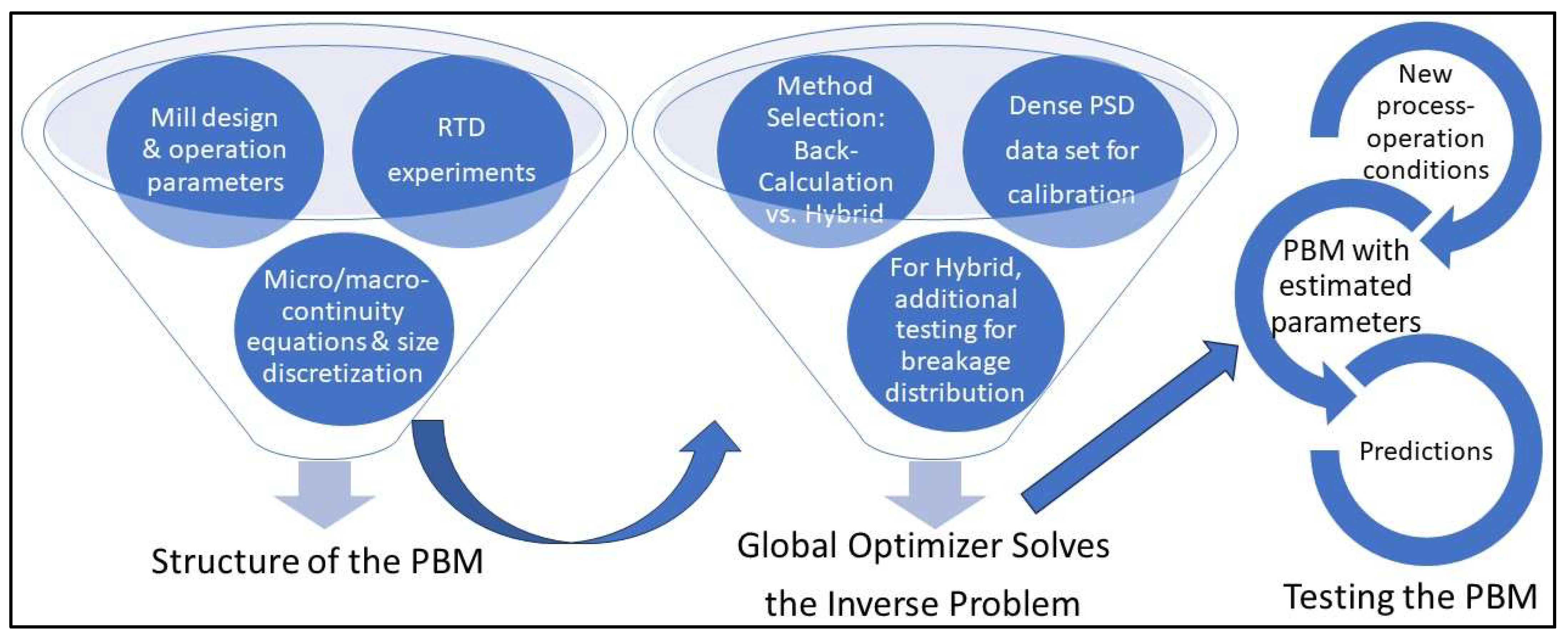
3. The Inverse Problem: Estimation of the PBM Parameters

The inverse problem entails estimating S_i, b_ij, or B_ij, as well as $d_i^{*}$if there is classification in the mill after the equipment design parameters and operating conditions are specified and a PBM is formulated mathematically (see Figure 1). The experimental PSD data must be gathered directly from the specific mill of interest. On the other hand, other (lab-scale) mills and drop-weight test instruments, as will be discussed below, can also be used to obtain breakage data in the hybrid (semi-back-calculation) method.

There are two major approaches to estimating the parameters and solving the inverse problem: “direct measurement methods” and “back-calculation methods” [4]. The former include the one-size fraction method [12] and the BI, BII, and BIII methods [13], respectively, and treat/fit experimental batch ball milling data. Without delving into details, the PBM is quite simplified in the limit of narrow feed sizes, which allow simple analytical solutions to estimate the unknown parameters. The pros/cons of these methods were extensively discussed by Austin et al. [4]. Another direct measurement approach is to find B_ij based on the breakage index t_n–t₁₀ family of curves. Here, t_n and t₁₀ refer to the percent of progeny particles that are finer than 1/nth and 1/10th, respectively, of the initial geometric mean size of the parent particles. These curves are constructed by characterizing materials via laboratory single-particle breakage tests and/or particle bed breakage in drop-weight tests or specialized comminution devices (see, e.g., [14,15,16]). All direct measurement methods entail the separate milling of multiple narrowly sized feed samples covering the size range of interest. Hence, they are experimentally time-consuming and expensive, some requiring specialized equipment/instruments. Importantly, while suitable for conventional ball milling [4], the one-size fraction method and the BI, BII, and BIII methods may not be accurately used for stirred media milling in fine milling applications as particle breakage is expected to be faster, which limits their applicability. Also, for fine milling and nanomilling applications, it is hard to prepare samples below <30 μm. Finally, all these methods yield information about S_i and B_ij of typically 3–8 size classes and apply interpolation–extrapolation to cover the whole size range and number of size classes of interest.

The (full) back-calculation method [10,17] aims to resolve the issues associated with the direct measurement methods, although it is plagued with other issues (non-uniquness and statistical insignificance). It typically uses a local optimizer along with the analytical or numerical solution of the PBM [6,8,9,10,17,18] to estimate the S_i and B_ij parameters simultaneously. The optimizer minimizes the sum-of-squared residuals SSR between the model-predicted PSD and the experimental PSD. However, a major challenge since the early applications of the back-calculation method is to find a unique set of statistically significant PBM parameters [4,8,9,10]. A local optimizer could get stuck at one of the local minima or hit a flat surface of the objective function, leading to an erroneous set of parameters despite yielding a deceptively reasonable fit to the specific set of PSD data. The non-uniqueness of the solution is revealed when the set of initial guesses for the parameters to be estimated is varied, which leads to different parameter estimates [8]. Unlike the direct measurement methods, the full back-calculation method has the advantage of general applicability to all milling processes as it is not bound by the size of the particles, the number of size classes, or the special equipment/instruments needed (e.g., for the t_n method). On the other hand, the semi-back-calculation (hybrid) method couples a direct measurement method with the back-calculation method and will be discussed in Section 3.2. As both the full back-calculation and semi-back-calculation (hybrid) methods use an optimizer to estimate PBM parameters, they are plagued with several common issues. Hence, the rest of this perspective article is largely dedicated to resolving the challenges associated with both types (full and semi) of the back-calculation methods, with the goal of minimizing the potential falsification of the estimated parameters. The direct measurement methods are too restrictive and limited, as discussed in the previous paragraph; their pros/cons have been extensively discussed in [4,12,13]. Hence, direct measurement methods are generally excluded from this perspective article unless otherwise indicated. Six principles have been given below, which have been implicitly implemented in refs. [8,9].

3.1. Principle I: Reduce Modeling Errors

No PBM can yield accurate parameters in the inverse problem if it does not account for key, fundamental physics such as relevant particle change mechanisms, either mechanistically or phenomenologically (modeling errors). In fact, this is the number one reason for falsified breakage kinetics [9,19,20]. Let us reconsider the underlying assumptions for the PBMs described in Equations (1)–(4). If the particles in the suspension/powder are prone to exhibit notable aggregation and particle growth, the use of Equations (1)–(4) in the inverse problem will lead to falsified breakage parameters. In the best case, this may become apparent in the deviations in the PBM-fitted PSDs from the experimental PSDs; in the worst case, the PBM may still provide a reasonable fit with some deviations. To minimize such modeling errors, two actions can be taken: (i) add the aggregation and/or particle growth terms to the PBM [21] or (ii) use stabilizers/dispersants in wet milling [22] and flow aids in dry milling to suppress aggregation–particle growth [23].

Another major modeling error is due to “non-linear breakage”, which is especially prevalent in dense suspension/powder systems during prolonged milling. The readers are referred to [24,25,26] for a comprehensive review of this phenomenon in various milling systems. Obviously, Equations (1)–(4) assume linear breakage or first-order breakage kinetics. Although the linear PBM yields reasonable fits to experimental batch milling data for short milling times, it exhibits notable deviations for prolonged milling [4,6]. In fact, short batch milling experiments have been commonly used to justify the first-order kinetics. Moreover, only short milling data can be used in the BI, BII, and BIII methods. When fitted to sufficiently long milling data, the non-linear effects become notable, and force-fitting the linear PBM led to falsified kinetics [9,19,20].

Another class of modeling errors pertains to deviations in the RTD of the particles in a particular continuous mill from the assumed RTD function in the PBM. For example, Equations (1)–(4) assume perfect mixing, which corresponds to an exponentially decaying RTD density function. However, perfect mixing is limited to short tubular mills (low L/D ratio) with fast radial–tangential mixing owing to the motion of the particles; such motion is usually generated by rotor-mixing elements, e.g., in a stirred media mill. Obviously, measuring the RTD in a particular mill via tracer studies [27,28] allows for quantifying the extent of imperfect mixing in continuous mills. Then, a more elaborate RTD model, such as the convection–dispersion model, the cell-based RTD model with recirculation between the cells, etc., can be used to formulate the PBM [29,30].

In the sequel, we consider milling processes wherein particle aggregation–growth is suppressed, perfect mixing in the mill is a reasonable approximation, and the mean residence time or retention time is not prolonged to cause the emergence of non-first-order effects. This practical approach is for illustrative purposes and discussion of the principles; however, the principles II–VI below are otherwise generally applicable to all milling processes. In fact, without the specific functional forms shown in the context of particle breakage–milling, the six principles are conceptually applicable to the PBM of other particulate processes such as granulations, aggregation, etc.

3.2. Principle II: Reduce the Number of Model Parameters

In the back-calculation method, the non-uniqueness of the estimated parameters and their statistical insignificance originate from the high number of breakage parameters and lack of sufficiently dense data sets with acceptable precision [8,31]; the latter aspect will be elaborated in Section 3.3. For a PBM with N size classes, there exist N S_i values, N $d_i^{*}$ values, and N(N–1)/2 values of B_ij. In the absence of classification, the total number of parameters equals (N² + N)/2; for example, 36 parameters must be estimated for an 8-size class PBM at a given (constant) set of process–design parameters! Clearly, a PBM with form-free S_i and B_ij parameters has little predictive capability. First, an 8-size class PBM has high size-discretization errors (Section 3.4); second, it is close to impossible to find them accurately with statistical significance because of the noise in the experimental milling tests.

Although direct fitting of form-free S_i and B_ij has been performed for a PBM with only a small number of size classes, the customary practice is to assume specific size-dependent functional forms and reduce the number of parameters drastically [4,10], such as the following:

$$S_i=A{\left(x_i/x_0\right)}^{\alpha }$$

(5)

$$B_{ij}={\varphi }_0{\left(\frac{x_{i-1}}{x_j}\right)}^{\gamma }+\left(1-{\varphi }_0\right){\left(\frac{x_{i-1}}{x_j}\right)}^{\beta }$$

(6)

where A, α, ϕ₀, γ, and β are the five fitting parameters, and x₀ is a normalizing reference size. Equation (6) is one of the most widely used B_ij in the ball milling literature and is known to be a size-normalized form [4]. Even these simplest forms have a total of five parameters. Clearly, assuming functional forms brings some bias to the modeling; hence, invoking specific functions should make use of prior knowledge of the specific mill–material, if available in the literature, and more preferably, several such models must be discriminated statistically based on the goodness-of-fit to experimental milling data and the statistical significance of the parameters (see, e.g., [9,10,20]) in the selection of the best model. For example, Equation (5) is known to be incapable of describing kinetics in ball milling, and Equation (6) cannot describe a non-normalized breakage distribution. In these cases, the following forms have been used [32,33,34]:

$$S_i=A{x}_i^{\alpha }{\left(x_{\mathrm{b},0}/x_{\mathrm{b}}\right)}^{\xi }{\left\{1+{\left[x_i/\left({\mu }_0{\left(x_{\mathrm{b}}/x_{\mathrm{b},0}\right)}^{\eta }\right)\right]}^{\Lambda }\right\}}^{-1}$$

(7)

$$B_{ij}={\varphi }_0{\left(\frac{x_{\mathrm{m}\mathrm{a}\mathrm{x}}}{x_j}\right)}^{\theta }{\left(\frac{x_{i-1}}{x_j}\right)}^{\gamma }+\left[1-{\varphi }_0{\left(\frac{x_{\mathrm{m}\mathrm{a}\mathrm{x}}}{x_j}\right)}^{\theta }\right]{\left(\frac{x_{i-1}}{x_j}\right)}^{\beta }$$

(8)

In Equations (7) and (8), ξ, μ₀, η, Λ, and θ are additional fitting parameters as compared to the parameters of Equations (5) and (6); x_b is the ball size; x_b,0 is a normalizing reference ball size; and x_max is the maximum particle size. When the normalization parameter θ equals 0, Equation (8) reduces to Equation (6). The total number of fitting parameters is 10. Note that while Equation (7) is capable of describing the impacts of ball size, it does not account for the impacts of rotation speed, ball filling, and powder loading in a ball mill. If these factors are multiplicatively added to Equation (7) in a power-law fashion to make the PBM more useful and predictive for practical applications (see Section 3.6), the number of parameters will increase to 13, at a minimum. An increase in the number of parameters causes more inaccurate estimation of the parameters, and the parameters may not be statistically significant besides the fact that a probable globally optimum solution will not be reached by optimization [8,9,10,31].

As per Principle I, a PBM must incorporate all the relevant physics either phenomenologically or mechanistically; so, Principle II does not suggest that we refrain from disregarding some mechanisms or aspects of breakage phenomena. Besides introducing size-dependent functional forms for S_i and B_ij, a major approach to reducing the parameters in the (full) back-calculation is the use of a hybrid method in which a direct measurement method such as BII (see, e.g., [35,36]) and the t_n–t₁₀ family of curves are used to estimate the parameters or matrix of B_ij separately and independently. Then, this B_ij is used along with the PSD data from the mill of interest to estimate S_i by back-calculation. Hence, although some of the issues associated with the full back-calculation method appear, the semi-back-calculation method reduces the number of parameters significantly and may become the best approach to the solution of the inverse PBM problem. The number of parameters to be fitted via semi-back-calculation is two, as opposed to five in Equations (5) and (6), and six, as opposed to ten in Equations (7) and (8).

A third major approach, which entails further research, is the reduction in PBM parameters through its one-way or two-way coupling with computational fluid dynamics (CFD) and the discrete element method (DEM) [37,38,39]. As an excellent demonstration of this point, for impact milling applications, Capece et al. [38,39] derived the specific breakage rate parameter S_i of the PBM, which differs from the arbitrary empirical breakage rate constants commonly employed in the milling literature, rigorously by augmenting the single-impact breakage model [40] and the impact energy spectra provided by DEM. They demonstrated that using only two material parameters of the single-impact breakage model, the specific breakage rate of the five-parameter Kotake–Kanda model [41], which was fitted to the experimental batch milling data, was reproduced by the DEM owing to the newly defined S_i function [39].

3.3. Principle III: Generate a Dense Data Set

The solution to the inverse problem dictates the availability of a sufficient number of experimental data, which are reproducible and relatively smooth, as a high number of PBM parameters are to be estimated. Taking multiple samples at various milling times, preferably separated at a geometric progression rather than a linear progression, in batch milling and multiple locations within the mill for continuously operating mills at multiple steady states are recommended. It is essential to take samples from multiple locations in the mill if particle classification is expected, for example, due to the presence of screens and diaphragms [42]. Also, to generate a dense data set, the use of laser diffraction is important as it provides PSD over 30–130 size classes. As sieving provides PSD information only for 5–10 size classes, a common practice is to combine it with some other sizing techniques to extend the PSD range to finer particles [8]. On-line and in-line sampling of PSD also enable engineers to build large data sets. In experimental measurements, care must be exercised to minimize sampling errors, and the precision of the measurements should be established. Unfortunately, one can even find studies that make use of 3-size-class PBMs, which are problematic partly because it is impossible to define a PSD with 3 size classes accurately, and the PBM is grossly inaccurate (see Principle IV).

3.4. Principle IV: Ensure a Grid-Independent Solution to the PBM

The accuracy of the PBM depends on the accuracy of the size discretization and the number of size classes used. In this perspective article, various discretization methods (in fact, solution methods) were excluded, as this topic deserves a separate perspective article (readers refer to [43]). Within the context of the simple, geometric discretization of the particle size domain implied in Equations (1)–(4), the use of a sufficiently large number of classes ensures one to find a non-changing solution, referred to as a grid-independent solution in CFD terminology. This aspect has been largely excluded from many milling studies in the minerals engineering literature, and it is not uncommon to find PBMs with 3–6 size classes, with little to no discussion of the errors involved. Austin [44] was the first to recognize that the use of 1/2^1/2 geometric progression, commonly used in sieving, could cause slight non-first-order behavior despite the linearity of the actual breakage kinetics. To describe the PSD more accurately and precisely, Principles III and IV go hand in hand; in general, dense data sets should be obtained from experiments. The PBM must be solved with a sufficient number of size classes, typically matching or exceeding the number of size classes in laser diffraction measurements, to provide grid-independent solutions or minimize discretization errors. In fact, one can and should solve the PBM with many size classes to obtain a grid-independent solution on a fine numerical grid and then reduce the PSD to the experimental size domain (typically a coarse grid) without incurring much error, as this would entail highly accurate interpolation on the fine grid (see [8,9] as examples).

3.5. Principle V: Use Global Optimization in Parameter Estimation

Even when Principle II is adopted in different ways to reduce the number of parameters, a useful PBM that accounts for the impacts of all process–design parameters is expected to have 5–10 parameters. Since the early inception of the full back-calculation method, local optimization has been commonly used to estimate the parameters [9,10,17,35]. Recent research [8,31] clearly established that when the number of PBM parameters is above a few, it is very difficult, if not impossible, to find a unique set of parameters via local optimization. The obtained solution may correspond to a local optimum [36] or a flat surface around an objective function [31]. The significant dependence of the optimization solution on the initial guess values of the parameters is a signature of its non-uniqueness. Hence, a global optimization algorithm, which is available in commercial software like MATLAB (the global optimization toolbox [45]) and Excel, should be used, preferably. For example, Muanpaopong et al. [8] used a non-linear constrained optimizer “fmincon”, coupled with the ODE solver “ode15s”, within the global optimization toolbox [45] of MATLAB, which minimized the sum-of-squared residuals SSR between the PBM-modeled PSD and the experimental PSD as the objective function. The MATLAB function “GlobalSearch” was used to generate the next set of initial guesses for the next trial point using the scatter search method [46]. Note that global optimization has been rarely used in the milling literature for estimating the parameters of the PBM within the context of the full or hybrid (semi-back-calculation) methods [8].

Principle V also recommends that the standard errors of the estimated parameters be reported and even the statistical significance of the parameters (p-values) be assessed. Interestingly, the early work on the full back-calculation method [4,10] emphasizes this aspect; however, this practice has rarely been adopted in the milling literature. Besides SSR and standard-error-of-residuals SER for assessing the goodness-of-fit, the standard error of the parameters SEP can be used to assess the statistical significance of the model parameters and even discriminate between alternative S_i and B_ij models [9,20]. To put it differently, while SSR and SER give an indication of how well the model fits the experimental data, SEP is an important statistic in determining the degree of certainty in the estimated parameters. A high SEP in comparison with the estimated parameter value indicates low certainty of the parameter estimate (or a wide confidence interval), which may be due to a lack of sufficiently accurate, dense data sets and/or the use of a poor model. SEP can be calculated by taking the square root of the diagonals of the parameter covariance matrix $\underset{\_}{\underset{\_}{\mathrm{C}}}$ determined at the back-calculated parameter set (${\underset{\_}{p}}^{\prime }$) [9], as detailed by Aster et al. [47] and shown in Equation (9).

$$\underset{\_}{\underset{\_}{\mathrm{C}}}\left({\underset{\_}{p}}^{\prime }\right)={SER}^2{\left[ {\underset{\_}{\underset{\_}{\mathrm{J}}}\left({\underset{\_}{p}}^{\prime }\right)}^{\mathrm{T}}\underset{\_}{\underset{\_}{\mathrm{J}}}\left({\underset{\_}{p}}^{\prime }\right)\right]}^{-1}$$

(9)

where T and –1 stand for matrix transpose and inverse operators, respectively. The Jacobian matrix $\underset{\_}{\underset{\_}{\mathrm{J}}}$ was also computed at the parameter set determined by the back-calculation method. Each row of the Jacobian matrix comprises the partial derivatives of the squared residual for a single experimental observation and model prediction with respect to each model parameter. Capece et al. [9] estimated the partial derivatives by using a first-order finite difference method also detailed by Aster et al. [47].

3.6. Principle VI: Test Predictive Capabilities of the PBM

A PBM is more than a fitting tool! Unfortunately, the way PBMs have been largely developed and used in the milling literature has germinated the wrong notion that PBMs can only be used to fit the spatiotemporal evolution of the experimental PSD data but not to predict the PSD evolution under different process–design conditions. This is partly related to the fact that most researchers do not take the next step of PBM validation in their studies, e.g., considering different feed PSDs, ball sizes, ball types, and processing conditions from those used in the model calibration step (parameter estimation). Obviously, a useful PBM should have a mathematical structure and robust parameter estimation to enable such predictions. For example, as written, a PBM with Equations (5) and (6) can only predict the impact of the changes in the feed PSD, whereas a PBM with Equations (7) and (8) can additionally predict the impact of various bead sizes/mixtures. To account for the impacts of various process parameters, the specific breakage rate parameter A of Equation (5) can be multiplicatively decomposed in the power-law form as follows:

$$A=A_0{p}_1^{a_1}{p}_2^{a_2}{p}_3^{a_3}$$

(10)

where p₁, p₂, and p₃ are three different process–design parameters, e.g., stirrer speed, ball density, and ball size in stirred media milling or similar process parameters in other milling processes [48,49]. The coefficient A₀ and the exponents a₁, a₂, and a₃ are additional fitting parameters. Other models that describe the dependence of S_i on process–design parameters have been established for tumbling ball milling [4]. Once calibrated, such a PBM can be used to predict the impact of the respective parameters. For example, Muanpaopong et al. [8] predicted the impact of a mixture of ball sizes and different feed PSDs on the batch milling of cement clinker, and such a feed PSD and ball mixture were not part of the parameter estimation.

4. Final Remarks

The author has presented six principles, within the context of back-calculation methods, to minimize falsified kinetics–breakage distribution in the PBM of milling processes, thus ultimately enabling the development of highly predictive and robust models. Ignoring several of these principles will almost guarantee that some parameters estimated are false and/or statistically insignificant, whereas consideration of all these principles will decrease the probability of the occurrence of falsified kinetics–breakage drastically.

An overarching assessment of the six principles is as follows: First and foremost, without a PBM that takes into account the key particle change mechanisms (Principle I), regardless of how accurately the remaining principles are implemented, the breakage kinetics and mechanisms will most likely be falsified. In other words, the falsification that originates from inadequate or wrong models cannot be compensated by using more accurate methods for solving the PBM, a global optimizer for parameter estimation, or comprehensive PSD data sets. While Principle I dictates the inclusion of the underling physics of milling processes and the general mathematical structure of the PBM, Principles II–IV will help to identify the minimum number of parameters that can be accurately determined with statistical significance. In terms of their significant impacts, these principles can be rank-ordered as follows: Principle II > Principle III > Principle IV. Principle II, along with Principle I, sets the total number of parameters estimated; hence, it is the most important among these three principles. While Principle III is only slightly less important than Principle II, it also sets some restrictions: the number of parameters cannot be more than the number of experimental data points; the number of numerical size classes should not be less than the number of experimental size classes. However, these restrictions are rather weak and thus rarely violated in practice. Principle IV weighs the least among the three principles because even a relatively crude size discretization (1/2^1/4 or even 1/2^1/2 to a smaller extent) can lead to a reasonable estimation of breakage parameters, as implied by Austin [9]. On the other hand, ref. [9] should be viewed with some caution because it is considered one of the simplest PBM structures, i.e., Equations (5) and (6). To ensure accurate parameter estimation and statistical significance, more elaborate PBMs with a higher number of parameters entail a denser data set and a finer size discretization. Finally, considering that even with the application of Principle II, a typical PBM has more than a few parameters, the full and semi-back-calculation methods entail using a global optimization scheme to find a probable globally optimal solution (Principle V). The local optimization schemes typically used in most PBM studies do not provide any assurance that a probable globally optimal solution (parameter estimates) has been found. Hence, Principle V is as important as Principle II. If used at all (see below for resources), Principle VI allows for validating the PBM and gives further assurance that significant falsification of breakage kinetics has not occurred. Overall, this perspective article suggests the following rank-ordering of all six principles: Principle I >> Principles II and V > Principle III > Principle IV > Principle VI.

The answer to the question posed in the title of this paper is, perhaps almost being a cliché: It depends! It depends on the number of parameters being estimated, the specific milling system–material being tested, the fidelity of the PBM to reality, the availability of dense, accurate, and precise experimental data for a large number of size classes, etc. In general, without considering specific cases, if Principles I, II, and V are disregarded, the PBM output will be falsified kinetics–breakage mechanisms regardless of the nature of the PSD data sets. On the other hand, it is unrealistic to expect that all six principles can be applied with the utmost mathematical rigor and excellence. In fact, the author is not aware of a single PBM study wherein all six principles have been perfectly applied in the milling literature. The formulation and implementation of PBMs also entails balancing various competing aspects besides scientific excellence: fit-for-purpose, availability and proper use of experimental–computational resources, and time and effort that can be dedicated. This latter point reflects the art-like elements of population balance modeling. In conclusion, this perspective article raises awareness of various challenges involved in the solution of the inverse PBM problem as pertinent to milling processes and provides researchers who want to use PBM with six principles to minimize falsified kinetics.

References

1. Randolph, A.D.; Larson, M.A. Theory of Particulate Processes; Academic Press: San Diego, CA, USA, 1988. [Google Scholar]
2. King, R.P. Modeling and Simulation of Mineral Processing Systems; Butterworth-Heinemann: Oxford, UK, 2001. [Google Scholar]
3. Prasher, C.L. Crushing and Grinding Process Handbook; Wiley: Chichester, UK, 1987. [Google Scholar]
4. Austin, L.G.; Klimpel, R.R.; Luckie, P.T. Process Engineering of Size Reduction: Ball Mill; Society of Mining Engineers of the AIME: Littleton, CO, USA, 1984. [Google Scholar]
5. Sedlatschek, K.; Bass, L. Contribution to the theory of milling processes. Powder Metall. Bull. 1953, 6, 148–153. [Google Scholar]
6. Austin, L.G. A review: Introduction to the mathematical description of grinding as a rate process. Powder Technol. 1971, 5, 1–17. [Google Scholar] [CrossRef]
7. Herbst, J.A.; Fuerstenau, D.W. Scale-up procedure for continuous grinding mill design using population balance models. Int. J. Miner. Process. 1980, 7, 1–31. [Google Scholar] [CrossRef]
8. Muanpaopong, N.; Davé, R.; Bilgili, E. A comparative analysis of steel and alumina balls in fine milling of cement clinker via PBM and DEM. Powder Technol. 2023, 421, 118454. [Google Scholar] [CrossRef]
9. Capece, M.; Bilgili, E.; Dave, R. Identification of the breakage rate and distribution parameters in a non-linear population balance model for batch milling. Powder Technol. 2011, 208, 195–204. [Google Scholar] [CrossRef]
10. Klimpel, R.R.; Austin, L.G. The back-calculation of specific rates of breakage and non-normalized breakage distribution parameters from batch grinding data. Int. J. Miner. Process. 1977, 4, 7–32. [Google Scholar] [CrossRef]
11. Whiten, W.J. A matrix theory of comminution machines. Chem. Eng. Sci. 1974, 29, 589–599. [Google Scholar] [CrossRef]
12. Austin, L.G.; Bhatia, V.K. Experimental methods for grinding studies in laboratory mills. Powder Technol. 1972, 5, 261–266. [Google Scholar] [CrossRef]
13. Austin, L.G.; Luckie, P.T. Methods for determination of breakage distribution parameters. Powder Technol. 1972, 5, 215–222. [Google Scholar] [CrossRef]
14. Palaniandy, S. Extending the application of JKFBC for gravity induced stirred mills feed ore characterization. Miner. Eng. 2017, 101, 1–9. [Google Scholar] [CrossRef]
15. Shi, F.N.; Kojovic, T. Validation of a model for impact breakage incorporating particle size effect. Int. J. Miner. Process. 2007, 82, 156–163. [Google Scholar] [CrossRef]
16. Napier–Munn, T.J.; Morrell, S.; Morrison, R.D.; Kojovic, T. Mineral Comminution Circuits—Their Operation and Optimization; JKMRC Monograph Series in Mining and Mineral Processing; Julius Kruttschnitt Mineral Research Centre, University of Queensland: Brisbane, Australia, 1996. [Google Scholar]
17. Devaswithin, A.; Pitchumani, B.; de Silva, S.R. Modified back-calculation method to predict particle size distributions for batch grinding in a ball mill. Ind. Eng. Chem. Res. 1988, 27, 723–726. [Google Scholar] [CrossRef]
18. Reid, K.J. A solution to the batch grinding equation. Chem. Eng. Sci. 1965, 20, 953–963. [Google Scholar] [CrossRef]
19. Capece, M.; Bilgili, E.; Dave, R. Emergence of falsified kinetics as a consequence of multi-particle interactions in dense-phase comminution processes. Chem. Eng. Sci. 2011, 66, 5672–5683. [Google Scholar] [CrossRef]
20. Bilgili, E.; Capece, M.; Afolabi, A. Modeling of milling processes via DEM, PBM, and microhydrodynamics. In Predictive Modeling of Pharmaceutical Unit Operations, 1st ed.; Pandey, P., Bharadwaj, R., Eds.; Elsevier: Oxford, UK, 2017; pp. 159–203. [Google Scholar]
21. Sommer, M.; Stenger, F.; Peukert, W.; Wagner, N.J. Agglomeration and breakage of nanoparticles in stirred media mills—A comparison of different methods and models. Chem. Eng. Sci. 2006, 61, 135–148. [Google Scholar] [CrossRef]
22. Peltonen, L.; Hirvonen, J. Pharmaceutical nanocrystals by nanomilling: Critical process parameters, particle fracturing, and stabilization methods. J. Pharm. Pharmacol. 2010, 62, 1569–1579. [Google Scholar] [CrossRef] [PubMed]
23. Toprak, N.A.; Benzer, A.H. Effects of grinding aids on model parameters of a cement ball mill and an air classifier. Powder Technol. 2019, 344, 706–718. [Google Scholar] [CrossRef]
24. Bilgili, E.; Scarlett, B. Population balance modeling of non-linear effects in milling processes. Powder Technol. 2005, 153, 59–71. [Google Scholar] [CrossRef]
25. Bilgili, E.; Yepes, J.; Scarlett, B. Formulation of a non-linear framework for population balance modeling of batch grinding: Beyond first-order kinetics. Chem. Eng. Sci. 2006, 61, 33–44. [Google Scholar] [CrossRef]
26. Capece, M.; Dave, R.N.; Bilgili, E. On the origin of non-linear breakage kinetics in dry milling. Powder Technol. 2015, 272, 189–203. [Google Scholar] [CrossRef]
27. Heitzmann, H. Caractérisation des Opérations de Dispersion—Broyage: Cas d’un Broyeur a Billes Continu Pour des Dispersions de Pigments. Ph.D. Thesis, Institut National Polytechnique de Lorraine, Nancy, France, 1992. [Google Scholar]
28. Kelsall, D.F.; Reid, K.J.; Stewart, P.S.B. A study of grinding processes by dynamic modelling. Electr. Eng. Trans. Inst. Eng. 1969, EE5, 155–169. [Google Scholar]
29. Kwade, A.; Schwedes, J. Wet grinding in stirred media mills. In Handbook of Powder Technology; Salman, A.D., Ghadiri, M., Hounslow, M.J., Eds.; Elsevier: Oxford, UK, 2007; pp. 253–380. [Google Scholar]
30. Fadhel, H.B.; Frances, C.; Mamourian, A. Investigations on ultra-fine grinding of titanium dioxide in a stirred media mill. Powder Technol. 1999, 105, 362–373. [Google Scholar] [CrossRef]
31. Kwon, J.; Cho, H. Investigation of error distribution in the back-calculation of breakage function model parameters via nonlinear programming. Minerals 2021, 11, 425. [Google Scholar] [CrossRef]
32. Austin, L.G.; Shoji, K.; Luckie, P.T. The effect of ball size on mill performance. Powder Technol. 1976, 1, 71–79. [Google Scholar] [CrossRef]
33. Austin, L.G.; Luckie, P.T. The estimation of non-normalized breakage distribution parameters from batch grinding tests. Powder Technol. 1972, 5, 267–271. [Google Scholar] [CrossRef]
34. Katubilwa, F.M.; Moys, M.H. Effect of ball size distribution on milling rate. Miner. Eng. 2009, 15, 1283–1288. [Google Scholar] [CrossRef]
35. Klimpel, R.R.; Austin, L.G. Determination of selection–for–breakage functions in the batch grinding equation by nonlinear optimization. Ind. Eng. Chem. Fundam. 1970, 9, 230–237. [Google Scholar] [CrossRef]
36. Zhang, Y.M.; Kavetsky, A. Investigation of particle breakage mechanisms in a batch ball mill using back-calculation. Int. J. Miner. Process. 1993, 39, 41–60. [Google Scholar] [CrossRef]
37. Carvalho, R.M.; Oliveira, A.L.R.; Petit, H.A.; Tavares, L.M. Comparing modeling approaches in simulating a continuous pilot– scale wet vertical stirred mill using PBM–DEM–CFD. Adv. Powder Technol. 2023, 34, 104–135. [Google Scholar] [CrossRef]
38. Capece, M.; Bilgili, E.; Dave, R.N. Formulation of a physically motivated specific breakage rate parameter for ball milling via the discrete element method. AIChE J. 2014, 60, 2404–2415. [Google Scholar] [CrossRef]
39. Capece, M.; Bilgili, E.; Davé, R. Insight into first–order breakage kinetics using a particle-scale breakage rate constant. Chem. Eng. Sci. 2014, 117, 318–330. [Google Scholar] [CrossRef]
40. Vogel, L.; Peukert, W. Breakage behaviour of different materials–Construction of a mastercurve for the breakage probability. Powder Technol. 2003, 129, 101–110. [Google Scholar] [CrossRef]
41. Kotake, N.; Suzuki, K.; Asahi, S.; Kanda, Y. Experimental study on the grinding rate constant of solid materials in a ball mill. Powder Technol. 2002, 122, 101–108. [Google Scholar] [CrossRef]
42. Genc, O. Optimization of an industrial scale open circuit three-compartment cement grinding ball mill with the aid of simulation. Int. J. Miner. Process. 2016, 154, 1–9. [Google Scholar] [CrossRef]
43. Ramkrishna, D. Population Balances–Theory and Applications to Particulate Systems in Engineering; Academic Press: San Diego, CA, USA, 2000. [Google Scholar]
44. Austin, L.G. A discussion of equations for the analysis of batch grinding data. Powder Technol. 1999, 106, 71–77. [Google Scholar] [CrossRef]
45. The MathWorks, Inc. Global Optimization Toolbox User’s Guide (R2022a); The MathWorks, Inc.: Natick, MA, USA, 2022. [Google Scholar]
46. Glover, F. A template for scatter search and path relinking. In Artificial Evolution, Lecture Notes in Computer Science; Hao, J.K., Lutton, E., Ronald, E., Schoenauer, M., Snyers, D., Eds.; Springer: Berlin/Heidelberg, Germany, 1998; Volume 1363, pp. 13–54. [Google Scholar]
47. Aster, R.; Borchers, B.; Thurber, C. Parameter Estimation and Inverse Problems; Elsevier Academic Press: Oxford, UK, 2005. [Google Scholar]
48. Tuzun, M.A. A Study of Comminution in a Vertical Stirred Ball Mill. Ph.D. Thesis, University of Natal, Durban, South Africa, 1993. [Google Scholar]
49. Hasan, M.; Palaniandy, S.; Hilden, M.; Powell, M. Calculating breakage parameters of a batch vertical stirred mill. Miner. Eng. 2017, 111, 229–237. [Google Scholar] [CrossRef]
Figure 1. A general scope of work required for formulating a PBM of a milling process, solving the inverse problem (parameter estimation via either the full back-calculation method or the semi-back-calculation/hybrid method), and testing–validating the PBM.
Powders 03 00012 g001
Disclaimer/Publisher’s Note: The statements, opinions and data contained in all publications are solely those of the individual author(s) and contributor(s) and not of MDPI and/or the editor(s). MDPI and/or the editor(s) disclaim responsibility for any injury to people or property resulting from any ideas, methods, instructions or products referred to in the content.