Investigation of Multidimensional Fractionation in Microchannels Combining a Numerical DEM-LBM Approach with Optical Measurements

Abstract

The fractionation in microchannels is a promising approach for the delivery of microparticles in narrow property distributions. The underlying mechanisms of the channels are however often not completely understood and are therefore subject to current research. These investigations are done using different numerical and experimental methods. In this work, we present and evaluate our method of combining a numerical Discrete Element Method (DEM)-Lattice Boltzmann Method (LBM) approach with experimental long-exposure fluorescence microscopy, micro-Particle Image Velocimetry (µPIV) and Astigmatism Particle Tracking Velocimetry (APTV) measurements. The suitability of the single approaches and their synergies are evaluated using the exemplary investigation of multidimensional fractionation in different channel geometries. It shows that both, numerical and experimental method are well suited to evaluate particle dynamics in microchannels. As they furthermore show strengths canceling out weaknesses of the respective other method, the combined method is very well suited for the comprehensive analysis of particle dynamics in microchannels.

1. Introduction

In order to supply micro-particles with defined narrow property distributions, suited fractionation methods are needed. One class of fractionation methods, which have shown to be able to fractionate microparticles by single properties such as size (see e.g., [1,2,3,4,5]), density (see e.g., [3]) or deformability (see e.g., [6]) but also multidimensionally (see e.g., [1,3]) are microfluidic fractionation methods. There is a plethora of different systems, which are however often still subject of current research. In this work we investigate Deterministic Lateral Displacement (DLD) channels (see e.g., [1,7,8,9]), serpentine channels (see e.g., [3,10,11]) and Multi-Orifice Flow Fractionation (MOFF) channels (see e.g., [5,12]).

There are two ways to investigate fluid and particles in microchannels: Experimental and numerical investigations. Unfortunately, they both suffer from distinct shortcomings such as the often high cost of channels (experimental) or the uncertainty whether all relevant effects have been considered (numerical). The approaches however tend to complement each other. For example in experimental investigations it is often very challenging to determine particle positions over channel height, which is simple when working numerically. On the other hand the investigation of a whole system including sidewall induced effects is simple when done experimentally but often computationally too expensive in resolved numerical simulations. Combining the methods therefore adds value to the conducted research.

Our goal is to highlight the advantages of a combined numerical and experimental approach. After an introduction to the used numerical (DEM-LBM) and experimental (µPIV, long-exposure fluorescence microscopy and APTV) methods (see Section 2) we will therefore give a short introduction into the investigated microchannels (see Section 3) and then show results. Those demonstrate not only the potential of the single methods for the investigation of microparticle fractionation, but especially the synergies between numerical and experimental methods of investigation (see Section 4).

2. Methods

In the following the numerical and experimental methods will be introduced. As detailed descriptions of both general methods and the respective used algorithms have been published in our previous works (see [1,3,10]), this paragraph contains only a brief introduction to the subject.

2.1. Numerical Methods

On the numerical side, we use a fully coupled combination of the Lattice Boltzmann Method (LBM) and the Discrete Element Method (DEM). Both used algorithms are in-house codes, which have been extensively tested and applied in previous studies (see e.g., [13,14,15,16,17] for DEM and [18,19,20,21,22] for LBM).

LBM is a relatively young CFD method, which works on a lattice in space [23] with a lattice spacing $\Delta x$. Its basic quantity are so called probability distribution functions $f_i\left(\mathit{r},t\right)$, which are defined on the nodes of the lattice and exist only for a set of discrete velocities ${\mathit{e}}_i$ [23]. In each time step, the distribution functions undergo a propagation step, bringing them to a neighboring node (depending on their respective velocity ${\mathit{e}}_i$), and then a collision step. The basic equation can be written as [24]:

$$\mathit{f}\left(\mathit{r}+{\mathit{e}}_i\Delta t,t+\Delta t\right)=\mathit{f}\left(\mathit{r},t\right)+\mathsf{\Delta }\left(\mathit{r},t\right),$$

(1)

with $\mathsf{\Delta }\left(\mathit{r},t\right)$ being the so called collision operator. If distribution functions would be propagated into solids such as particles or channel walls, bounce-back methods are in our case used to calculate the reflected distributions (see [1] for details on the implementation and [25] for details on the methodology in general). These realize not only the flow around the particles and channel structures, but furthermore no-slip boundary conditions on the respective surfaces [26] through which particle rotations affect the surrounding fluid. The hydrodynamic force and torque exerted on particles and walls is in our case determined through so called momentum exchange methods (see [1] for details on the implementation and [27] for details on the methodology in general).

A deeper insight to the used D3Q19 model as well as bounce back-methods, forcing algorithm and collision operator can be found in [1,3]. We use LBM to simulate the flow in the investigated microchannel geometries and determine fluid forces and torques, which are exerted onto the particles in each time step. LBM is done in dimensionless so called lattice units [23]. Before giving the values to the DEM, they therefore need to be converted into physical units (see [23] for details). The physical values are then given to the DEM, which uses them in the calculation of particle positions and velocities.

The Discrete Element Method is used to calculate dynamics of particulate systems (see e.g., [13,15,16,17]). It uses Newton’s second law of motion to determine particle positions and velocities based on the respective attacking forces [28]. In our case the main equations read:

$$m_P\frac{d^2\mathit{x}}{d{t}^2}={\mathit{F}}^c+{\mathit{F}}^{pf}+{\mathit{F}}^g,$$

(2)

$$I_P\frac{d{\mathit{\omega }}_P}{dt}={\mathit{T}}^{pf}+{\mathit{T}}^c,$$

(3)

with $\mathit{x}$ being the particle positions, $m_P$ the particle masses, ${\mathit{\omega }}_P$ the rotational velocities, $I_P$ the particle inertias and $\mathit{F}$ and $\mathit{T}$ forces and torques. In our case forces and torques from fluid particle interaction (index $pf$), contacts (index $c$) and gravity (index $g$) are considered. We use a spring dashpot model to determine normal forces and a linear spring limited by the Coulomb condition for tangential forces. Further details on the implementation and the used set of parameters can be found in [1].

The workflow is thus as follows: Based on the flow conditions in the previous time step and the current particle locations and velocities (translational and rotational) LBM determines a new flow field. It then calculates forces and torques onto particles based on particle positions and velocities (translational and rotational) and the respective local flow conditions. Those values are then converted from lattice to physical units and transferred to the DEM. DEM calculates contact forces and torques based on particle-particle and/or particle-wall contacts. DEM then calculates new particle positions and velocities (translational and rotational) based on forces and torques from fluid-particle interaction and from contact events. Those values are converted from physical to lattice units and transferred to the LBM (see also algorithm flowchart in [3]).

It has to be noted, that LBM can be computationally relatively expensive when resolving flow around individual particles. To deal with this, it is common practice, to work with periodic boundary conditions if the system structure allows it (see e.g., [6,20,29]). In our case this means that we simulate for example only one serpentine element of the serpentine channel and particles leaving the element at its outlet reenter it at the inlet.

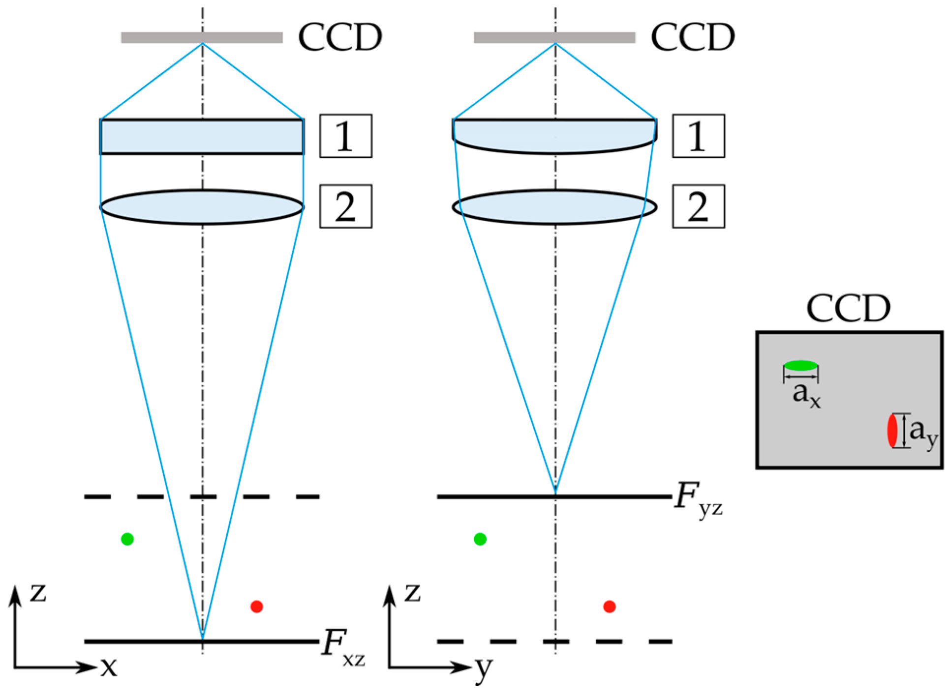
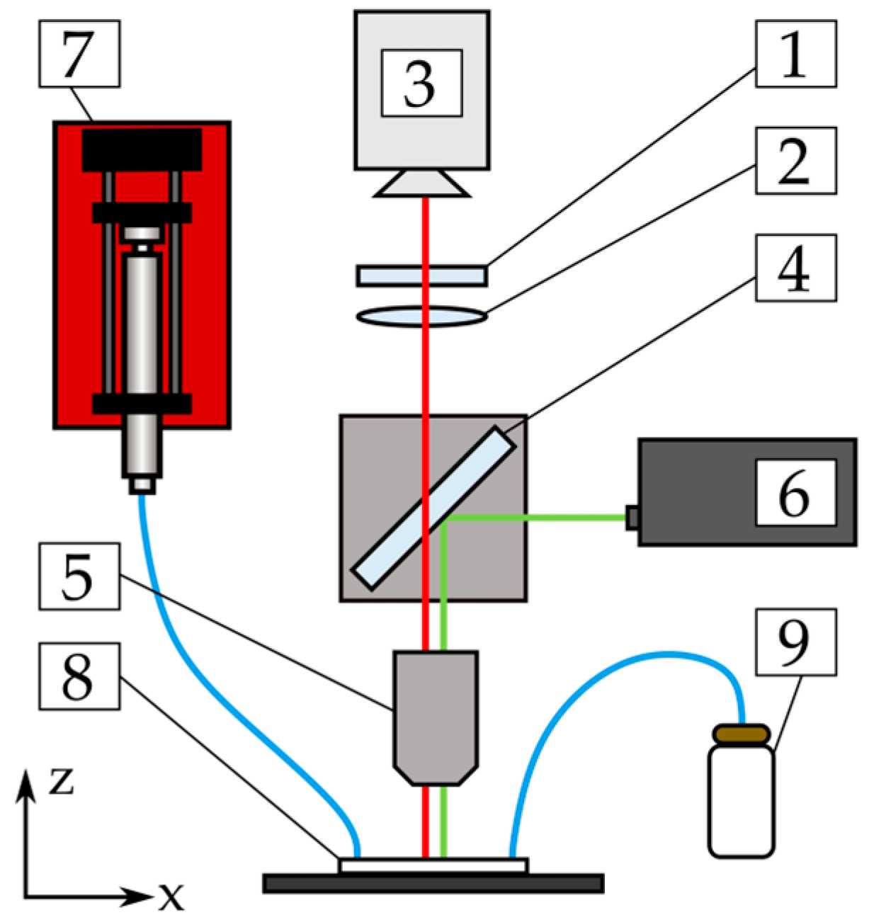
2.2. Experimental Methods

The experiments are conducted using a microfluidic chip of 45 mm $\times$ 15 mm $\times$ 1.38 mm produced by Micronit GmbH, (Enschede, the Netherlands) (see Figure 1). The microfluidic channel geometries are fabricated by a deep reactive ion-etching (DRIE) process in silicon wafers. For optical accessibility, glass is bonded on top of the silicon base. The chip contains a Multi-Orifice Flow Fractionation (MOFF) channel, a Deterministic Lateral Displacement (DLD) channel, a square wave serpentine channel and the necessary in- and outlets to operate them.

Particle equilibria are investigated by means of APTV and long-exposure fluorescence microscopy. The latter uses a continuous white light halogen lamp for illumination and a CCD camera to record particle images with an exposure time of one second. More details on the specifications of the used devices and the experimental set-up can be found in [30].

We conduct micro-Particle Image Velocimetry (µPIV) measurements to provide the velocity fields of the flow and Astigmatism Particle Tracking Velocimetry (APTV) to reconstruct 3D particle positions and motion in the flow. Flow results obtained from µPIV can be utilized to validate numerically determined results (see e.g., [30]). Furthermore, 3D particle distributions obtained from APTV measurements can be utilized to validate the particle trajectories that are numerically determined by coupling DEM to LBM. This provides opportunities for a deeper analysis of particle dynamics also in complex channel geometries.

Astigmatism Particle Tracking Velocimetry (APTV) is a single camera technique to measure all three components of a particles position as well as the corresponding velocity components [31,32]. Kao et al. [33] conducted measurements to track single fluorescent particles by introducing a cylindrical lens in the light path, thus using the astigmatism effect. Cierpka et al. [32] proposed an intrinsic calibration method based on the measurement itself, so that all image aberrations, including the distortions in the x-y plane, are taken into account. Using this intrinsic calibration procedure, reconstruction errors of less than 1 µm in z-direction have been reached for particles with diameters of 2 µm and 5 µm [32].

The principle of the APTV method is illustrated in Figure 2: A (1) cylindrical lens is placed between (2) the field lens and the CCD chip of the camera to produce an aberrated particle image. The cylindrical lens acts as a flat lens in the x-z plane therefore having a negligible effect on the path of the light emitted by the fluorescent particles, while the light path is significantly affected by the curvature of the cylindrical lens in the y-z plane.

This results in two separated focus planes $F_{\mathrm{x}\mathrm{z}}$ and $F_{\mathrm{y}\mathrm{z}}$ on the object side. If the particle is located in the middle between these focus planes it assumes a slightly blurred, rather circular shape. Otherwise, an elliptical particle image is created in the image plane. Corresponding to the mounting position shown in Figure 2, the shorter axis of the elliptical image is oriented along the x- or y-axis, depending on whether the particle is located closer to the $F_{\mathrm{x}\mathrm{z}}$ or $F_{\mathrm{y}\mathrm{z}}$ plane. After applying an auto-correlation algorithm, the major and minor axis lengths $a_{\mathrm{x}}$ and $a_{\mathrm{y}}$ of the auto-correlation peak are determined. The ratio $a_{\mathrm{x}}/a_{\mathrm{y}}$ is a measure for the relative z position of the particle in the measurement volume [31,32]. To determine the correct z positions of particles, an in-situ calibration preceding the actual measurement is required with a set of particles located at known positions. Usually, a set of sedimented particles located at the channel bottom is utilized for the calibration procedure. Details on the applied calibration and evaluation procedure can be found in Blahout et al. [10].

A sketch of the used experimental set-up is shown in Figure 3. The optical set-up includes (1) a cylindrical lens with a focal length of $f_c=200$ mm, (2) a field lens, (3) a dual-frame CCD camera (LaVision Imager pro SX, LaVision, Göttingen, Germany), (4) a dichroic mirror (Nikon G-2A filter set, Nikon, Tokyo, Japan) and (5) an objective with lens of $M=20$ (Nikon CFI60, Nikon, Tokyo, Japan) mounted to an epifluorescence microscope (Nikon Eclipse LV 100, Nikon, Tokyo, Japan). Illumination at a wavelength of $\lambda =532$ nm is provided by (6) a double-pulsed laser (Litron Nano S 65-15 PIV, Litron, Rugby, England), and then reflected by (4) the dichroic mirror (green path in Figure 3) to excite the fluorescent particles (red path for emission in Figure 3) in (8) the microchannel (Micronit GmbH, see also Figure 1). The suspended particles are injected by (7) a syringe pump (HLL LA-800, Landgraf Laborsysteme HLL GmbH, Langenhagen, Germany) and finally collected in (9) a waste bottle.

We furthermore performed µPIV measurements (see [34,35,36] for details on the method). In contrast to conventional Particle Image Velocimetry (PIV) (see [37,38] for details on the method) here a volume in the fluid is illuminated instead of illumination by a light sheet. The volume illumination is caused by the imaging set-up, consisting of light source and camera, which are aligned on the same side of the channel. Similar to conventional PIV, a velocity field is determined using seeded tracer particles in a fluid [34]. Furthermore, also consecutive images separated by a certain time interval are recorded [34]. The recorded images are then segmented into sub-regions known as interrogation areas [37,38]. A cross-correlation algorithm is then applied on two successive images of each interrogation area to determine the respective fluid velocity based on the corresponding displacement field [39].

The experimental setup used for µPIV matches the APTV setup shown in Figure 2, just without the cylindrical lens. As the illumination of a volume element causes the respective out-of-plane particles to be illuminated as well and thus contribute to the background noise, certain peculiarities of µPIV have to be considered. First, illuminated but defocused particles contribute to the correlation result which may cause a bias to the flow result, especially when there is a flow gradient in out-of-plane direction. This can be quantified by the depth-of-correlation [40]. Furthermore, due to the volume illumination a lower particle image density has to be used compared to conventional PIV to reduce background noise [41]. Less particles however, lead to decreased detection probability [42]. To overcome this, ensemble averaging algorithms are utilized that average the correlation results in order to improve the reliability of flow field results [43].

2.3. Synergies

The synergy of numerical and experimental investigations is based on the fact that both methods have different advantages, which in most cases cancel out weaknesses of the respective other method, thus providing the possibility of comprehensive analyses at relatively low effort.

Advantages of experimental investigations are for example the automatic inclusion of phenomena such as surface effects, all relevant forces and Brownian motion without need for assumptions such as negligibility of certain ones. This is not automatically the case in numerical studies. Also system size and number and size of particles can be easily adjusted in an experiment. In numerical investigations on the other hand, the computational cost rises with system size and number of particles. Great size differences between particles and fluid phenomena can also be quite challenging in numerical investigations as the locally required high resolutions either lead to high computational cost or need to be realized through elaborate mechanisms such as dynamic local grid refinement. In experimental evaluation, this poses no problem.

Advantages of numerical investigations on the other hand are for example the availability of all values: Whilst some of the relevant values such as in plane positions are relatively easy to determine in experiment, others such as positions over depth or rotation can (if at all) only be determined with great effort. In the numerical investigation however, those values are easily available for all particles and time steps. Another advantage of numerical investigations is the flexibility when it comes to system parameters: Not only are channel geometries relatively simple to adjust (whilst in experiment, a new channel would need to be machined), the parameters of fluid and particles can furthermore be freely and independently adjusted in order to explore the effect of interest. In experiment on the other hand, one is limited not only to parameter combinations of real materials or mixtures, but furthermore to products which are commercially available or can be produced by oneself. This hold especially true for non-spherical particles, which can be relatively easy modeled in any shape for numerical investigations, whilst the shapes available for experimental investigations are quite limited. Lastly, in numerical investigations, all the relevant parameters are predefined, which prevents errors due to unforeseen environmental influences such as temperature changes affecting fluid viscosity or similar effects.

To sum up, one can say, that even though numerical and experimental investigations are both powerful methods in themselves, they both suffer from significant deficits. When combined however, those deficits cancel out which leads to great synergies.

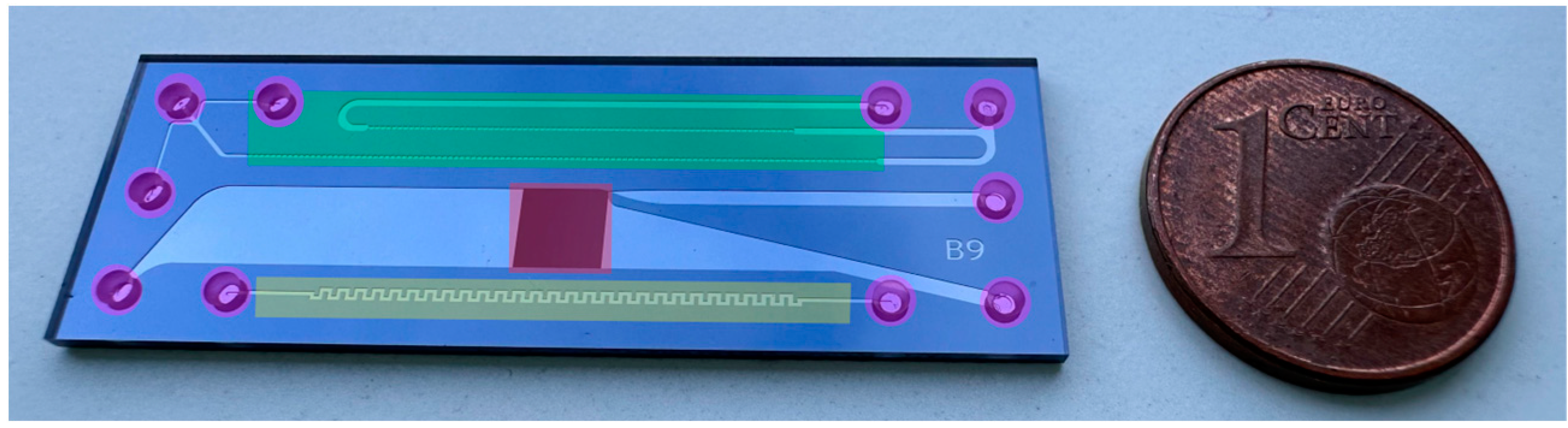
3. Investigated Microchannel Geometries

In the following, an overview of the functionality of the investigated microchannel geometries will be presented. An in depth analysis would go beyond the scope of this paper. More detailed information can however be found in e.g., [1,2,44] for fractionation through Deterministic Lateral Displacement, [3,10,11,30] for fractionation in serpentine channels and [5,12,45,46] for fractionation in Multi-Orifice Flow Fractionation channels.

3.1. Deterministic Lateral Displacement Channels

Deterministic Lateral Displacement (DLD) is a microfluidic fractionation method where particles and fluid are led though a periodic array of obstacles [2] (in the following referred to as pillars, as mostly cylinders (see e.g., [7,47,48,49]) or uniform prisms (see e.g., [50,51]) are used). Each pillar row is laterally shifted from the previous one by a certain distance. This leads to the effect that the flow through the system is split into several streams, which all hold the same volume flow and do not mix [2]. The shift is described through the row shift fraction $ϵ$, which equals the inverse of the number of partial streams [9].

Particles smaller than a threshold, the so called critical diameter (see e.g., [1,7,9]), will pass the system in one of the streams, following its zigzag path [2]. This mode is thus commonly called the zigzag mode (see e.g., [1,2,7]). Particles larger than the critical diameter will be displaced by every pillar row [2] and travel in a mode commonly titled as the bump- or displacement mode (see e.g., [1,2,9,44]). Some studies reported a third mode of transport, called mixed mode/motion (see e.g., [48,49,52]), which will however not be discussed here.

There are two basic DLD layouts: Rhombic (also called row shifted parallelogram) and tilted/rotated square arrays [44,48]. The splitting into partial streams and both modes of transport are schematically illustrated in Figure 4 for both geometries, each employing a row shift fraction $ϵ$ of 1/3.

An essential point when working with DLD channels is the prediction of the critical particle diameter $D_C$, which is why several correlations have been developed here. Shown in Figure 5 is the correlation $D_C=1.4\cdot G\cdot {ϵ}^{0.48}$ by Davis [53], which relates the critical diameter $D_C$ to the gap width $G$ as well as the row shift fraction $ϵ$ and is derived from experimental data. As mentioned above, particles below the critical diameter show a zigzag mode whilst particles above it show a bump mode.

It has to be noted that the classical DLD theory holds true only for low Reynolds numbers (see e.g., [8]). In order to explore the effects and possibilities arising from the operation at elevated Reynolds numbers, several studies have been performed on the topic during the last years, which found vortices forming behind the pillars (see e.g., [1,54,55]), influences on critical diameters (see e.g., [1,7,8]) and particle movement in terms of periodicities (see e.g., [1,55]) and the relevance of particle density (see e.g., [1]).

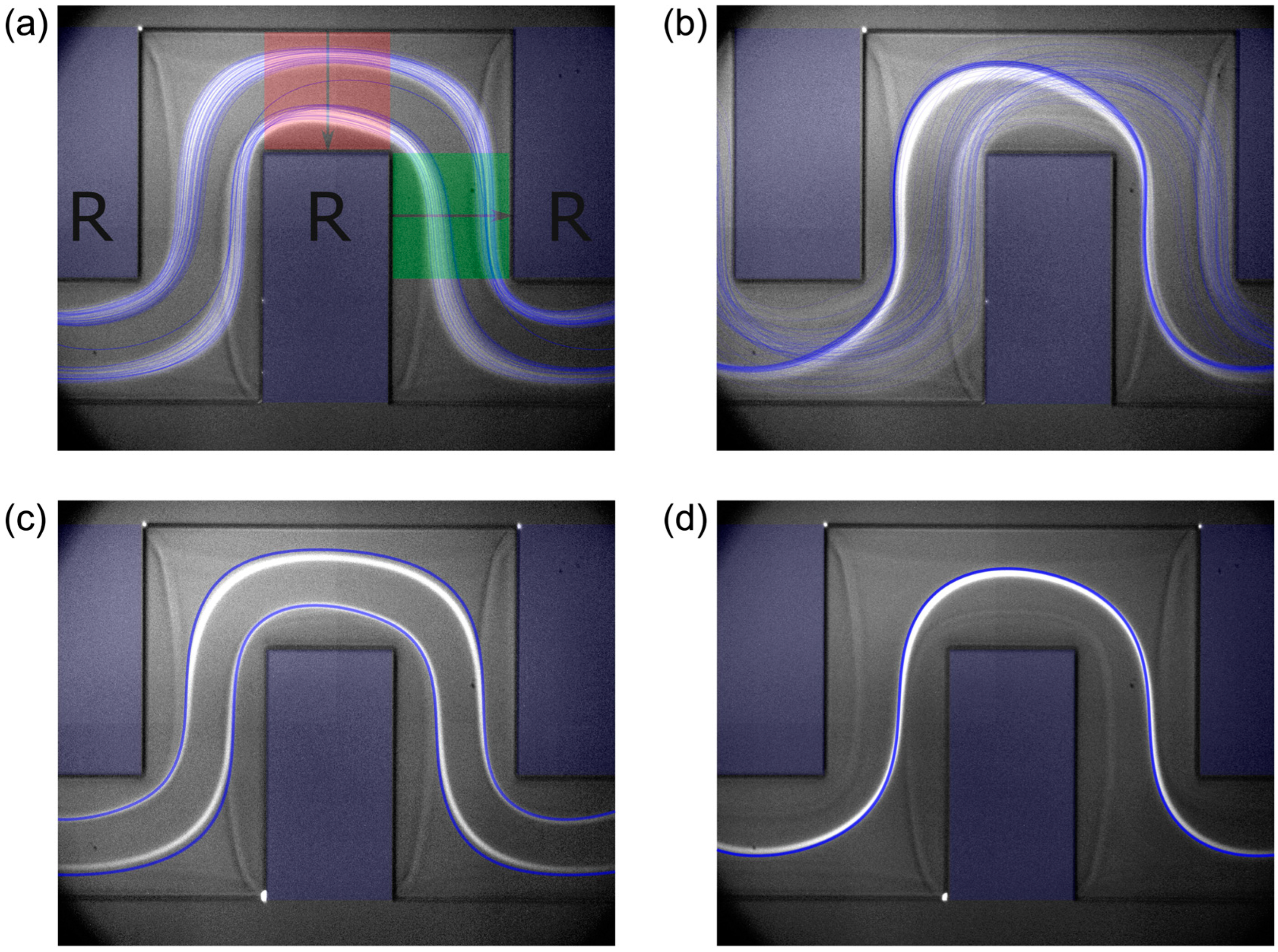
3.2. Serpentine Channels

Serpentine microchannels have become increasingly popular since Di Carlo et al. [56] investigated inertial focusing in symmetric and asymmetric geometries. Zhang et al. [11] later demonstrated that it is possible to focus particles down to a single streak over channel width in a symmetric serpentine channel. This effect can be exploited for particle fractionation by operating at conditions, where one type of particles shows one centered equilibrium streak over channel width whilst another one shows two equilibria near the channel walls (see e.g., [4]).

The focusing is said to depend on inertial lift forces ([4,56], see e.g., [57] for details on forces), centrifugal forces ([4,11]) and drag force exerted by Dean vortices ([4,56], see e.g., [58] for details on vortices), the mechanism is however so far not fully understood. Two aspects complicate the investigation: The first one is the fact that the acting forces strongly depend on the exact position of the particle in the channel. This means that, even for a particle on an equilibrium trajectory, they do not necessarily cancel out at each position, but merely over one periodic element of the channel geometry. The second one is that there is a plethora of serpentine channel geometries and it is not clear to what extent results taken in one geometry are valid for the other geometries as well. Investigated are for example square wave channels (see e.g., [3,4,10,30,59]), sinusoidal channels (see e.g., [56,60]), zigzag channels (see e.g., [59,61]), symmetric (see e.g., [3,56,59]) and asymmetric (see e.g., [56,62]) geometries.

Still the use of serpentine channels for the manipulation of microparticles is very attractive, as the channels have a simple linear structure (relatively easy fabrication and parallelization), do not rely on external forces and have proven to work with model particles as well as with cells (see e.g., [4,61,63,64,65]). All this makes serpentine channels very attractive, which is why they are the subject of current research.

In our studies (see [3,10,30]), we worked with a square wave serpentine channel (see Figure 6) and systematically investigated the influence of particle size and density on position and width of resulting equilibria over Reynolds number at different positions in the channel geometry.

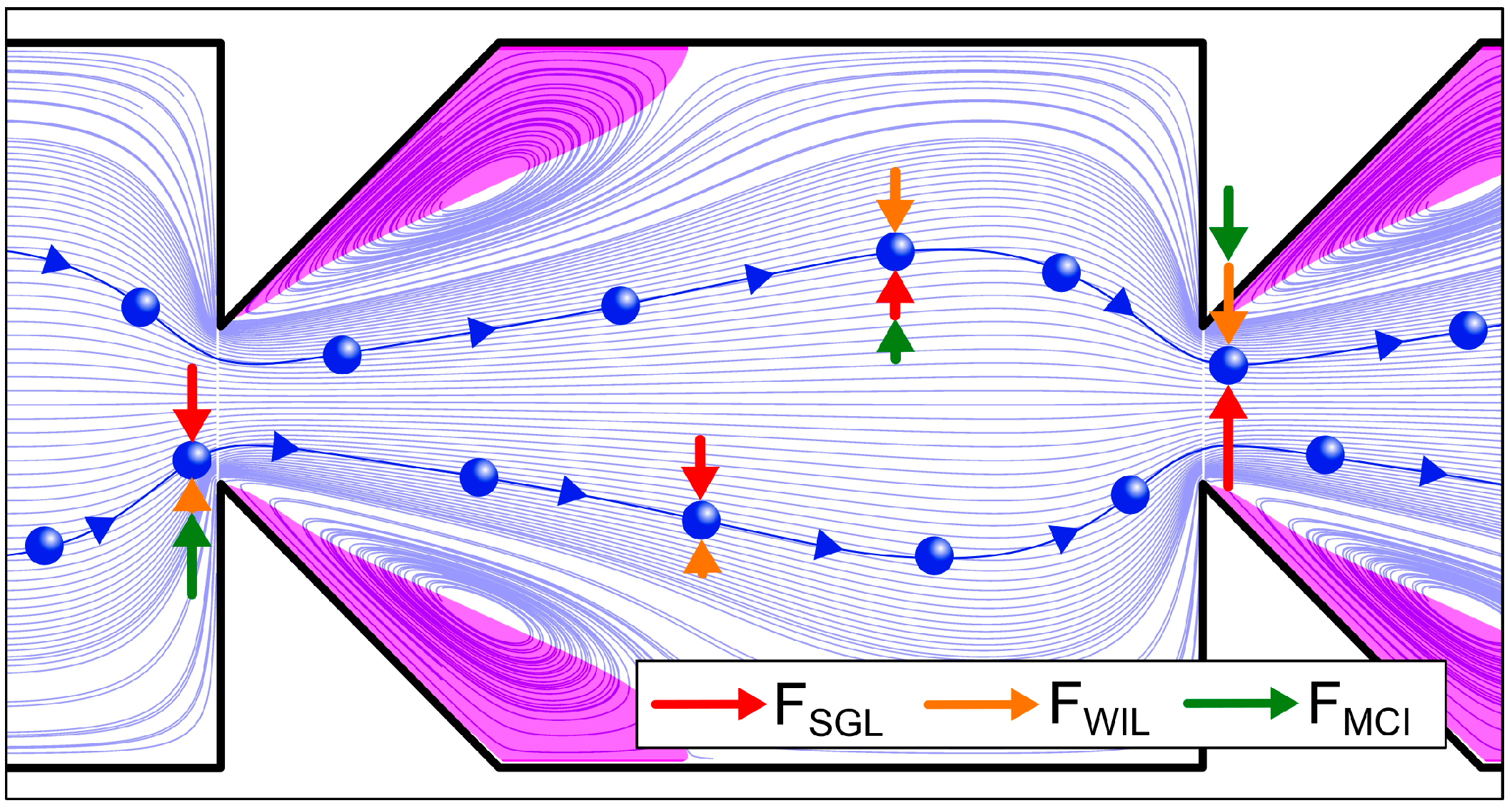
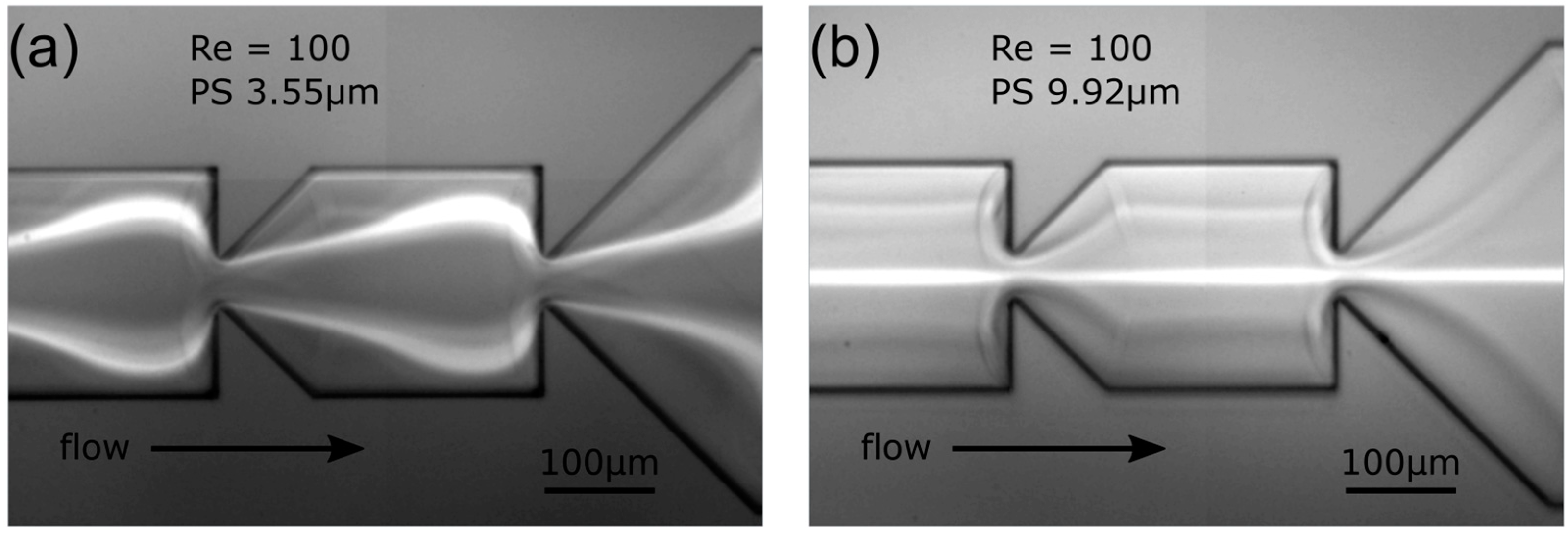
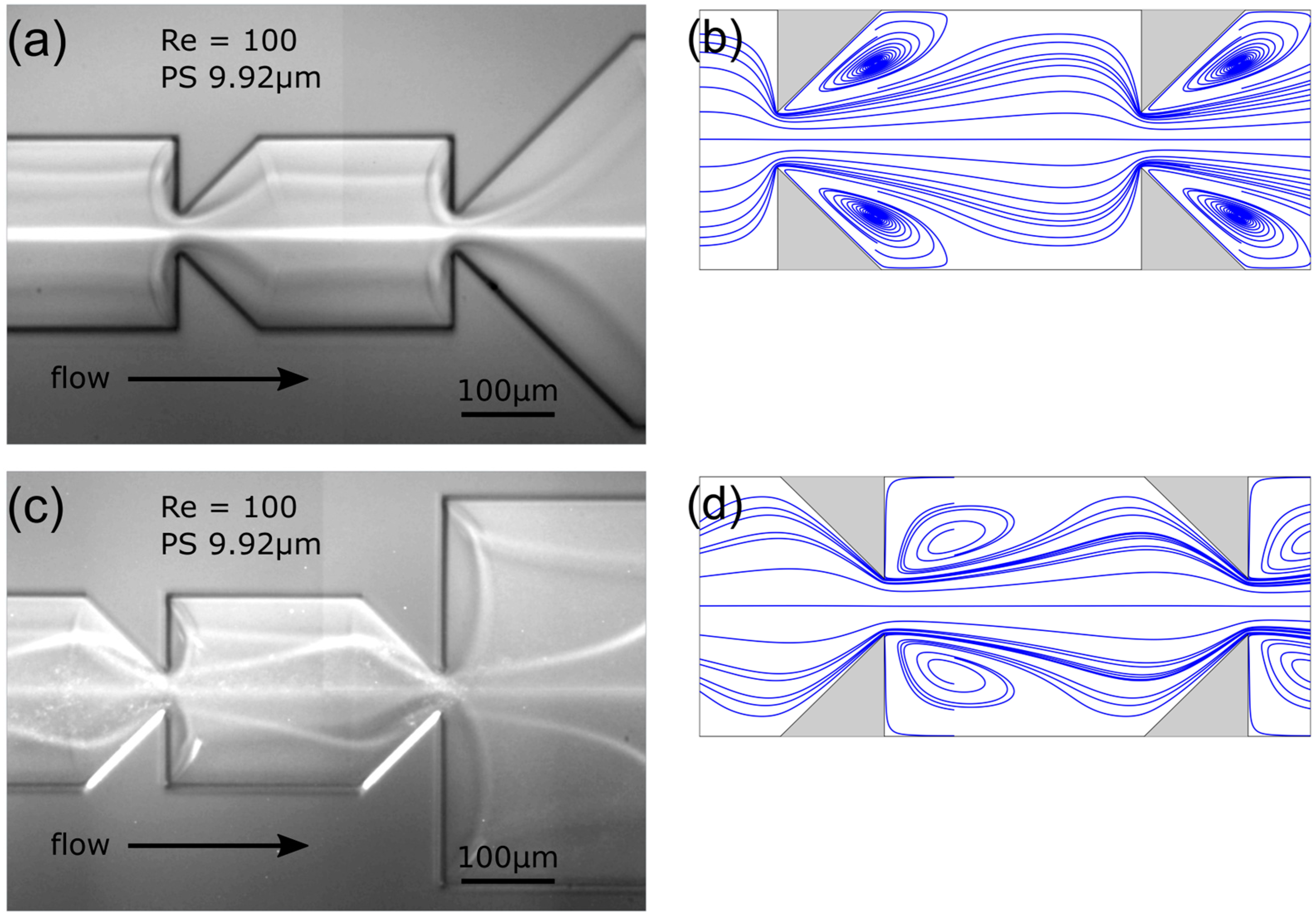
3.3. Multi-Orifice Flow Fractionation channels

Multi-Orifice Flow Fractionation (MOFF) is a continuous passive microfluidic fractionation method [12]. It is based on inertial effects in symmetrical contraction-expansion (Multi-Orifice) microchannels [12]. The method was introduced by Park et al. [46] who showed for those channels that particles can be focused [46] on equilibrium trajectories, with lateral equilibrium positions depending on Reynolds numbers [12,46] and particle size [12]. At a specific Reynolds number larger particles were focused close to the centerline, while smaller particles stayed on lateral equilibrium trajectories [12]. The spatial separation of the different-sized particles can then be used for fractionation by using multi-outlet systems (see e.g., [45,66]).

Following Park et al. [12], the effects responsible for the forming of equilibrium trajectories of the particles are momentum-change-induced inertial force (${\mathrm{F}}_{\mathrm{MCI}}$), shear-gradient induced lift force (${\mathrm{F}}_{\mathrm{SGL}}$) and wall-effect-induced lift force (${\mathrm{F}}_{\mathrm{WIL}}$), (see [12] for details). The interaction of these forces causes the focusing of particles on equilibrium trajectories at appropriate Reynolds numbers [12] (see Figure 7).

The originally proposed geometry by Park et al. [46] is a symmetric contraction-expansion array microchannel with a quadratic footprint for the expansion regions and the contraction regions being half as long and one fifth as wide [46]. Fan et al. [5] used another channel geometry but still used a symmetric contraction-expansion array microchannel with multiple orifices to fractionate by flow, which is why, in this publication we count Fan et al. [5] as using the MOFF-method. By introducing gradual expansions to the contraction regions (see Figure 7) Fan et al. [5] were able to achieve narrower particle bandwidth and higher separation distance (compared to the standard geometry with rectangular compartments) between particle streams at the outlet [5].

4. Results

In the following subsections, numerical and experimental results of the investigation of DLD- (Section 4.1), serpentine- (Section 4.2) and MOFF channels (Section 4.3) are presented. They demonstrate not only the suitability of the employed numerical (see Section 2.1) and experimental (see Section 2.2) methods, but especially their synergies.

4.1. Deterministic Lateral Displacement Channels

Especially for the investigation of Deterministic Lateral Displacement channels, the numerical investigation offers several significant advantages: (i) The geometry is highly periodic, so when working with periodic boundary conditions, only relatively small systems need to be considered. (ii) The possibility to work with periodic boundary conditions allows the investigation of the basic functionality without influences by channel walls. (iii) The fact that numerical investigations can be conducted using only one single particle makes clogging, (which can be a significant issue in experimental investigations) no problem. (iv) A comprehensive analysis of the phenomena requires the use of several different channel structures, which is where the numerical investigations are far more flexible than experimental investigations. Of course, the numerical methodology needs experimental validation, which can however in this case be done using experimental data from literature. Those are the reasons we started our investigations of DLD channels with the numerical side. Experimental investigations are in progress, but will need some time, which is why this section focuses on our numerical investigations.

Using the numerical methods specified in Section 2.1, we built a regular three times three pillar system with periodic boundary conditions and a depth of at least three particle diameters (see [1]). These dimensions proved to be enough to sufficiently prevent self-influencing of particles over the periodic boundaries [1]. Using a volume force attacking at different inclinations, we were able to simulate tilted square arrays of different periodicities and thereby row shift fractions $ϵ$. Calculations were done with different particle sizes, periodicities and Reynolds numbers. The results closely matched results published in literature for the critical diameter/particle behavior at low Reynolds numbers (compare [9,53,67]), the periodicity of particles at elevated Reynolds numbers (compare [55]) and the roughly linear decline of the normalized critical diameter with rising Reynolds number (compare [7,8]). The exact results can be found in Reinecke et al. [1].

Using the thus validated system, simulations were done to explore the influence of particle density at different Reynolds numbers. The results showed a density dependence of critical diameters, which rose with row shift fraction of the channel, density difference and Reynolds number, meaning that a density fractionation would be most promising at elevated Reynolds numbers and using a channel of low periodicity [1]. The results were then used to describe the relationship through:

$$D_C=G\cdot A\cdot {ϵ}^B\cdot \left(1-Re\cdot \left(C+D\cdot \frac{{\rho }_p{\mathrm{m}}^3}{1000 \mathrm{k}\mathrm{g}}\right)\right),$$

(4)

with the fitted parameters A through D (see [1]). This formula allows the prediction of critical diameters as a function of row shift fraction $ϵ$ and Reynolds number, which cannot only be used to fractionate for density, but allows for the fractionation of multiple fractions in one channel.

This is in the following exemplarily shown for a fractionation of particles of densities of 1050 (which is a common value for polystyrene, see e.g., [10,68,69]) and 1850 kg/m³ (which matches silica based microparticles, see [30]) and sizes of 5 and 6 µm into the four fractions. When assuming a channel with a constant gap width of 20 µm, and Reynolds numbers of 1 and 55, the critical diameters of the particles can be predicted as shown in Figure 8.

As described in Section 3.1, fractions are separated when one of them assumes a bump mode, whilst the other one assumes a zigzag mode. Assuming fractions of $D_1,{\rho }_1$ and $D_2,{\rho }_2$ this translates to $D_c\left({\rho }_1,\mathrm{R}\mathrm{e},ϵ\right)<D_1$ and $D_c\left({\rho }_2,\mathrm{R}\mathrm{e},ϵ\right)>D_2$ or vice versa. Based on this, and using the relationships shown in Figure 8, the fractionation of particles of diameters of 5 and 6 µm and densities of 1050 and 1850 kg/m³ into the four fractions can be done in three steps, equaling to three different channel sections with different parameters Re and $ϵ$:

• Re = 1 (critical diameters in turquoise and orange scatter with black line in Figure 8); $ϵ$ = 1/36 (blue dotted vertical line in Figure 8): At this operating point the larger particles of both densities lie above their critical diameters and thus show a bump mode;
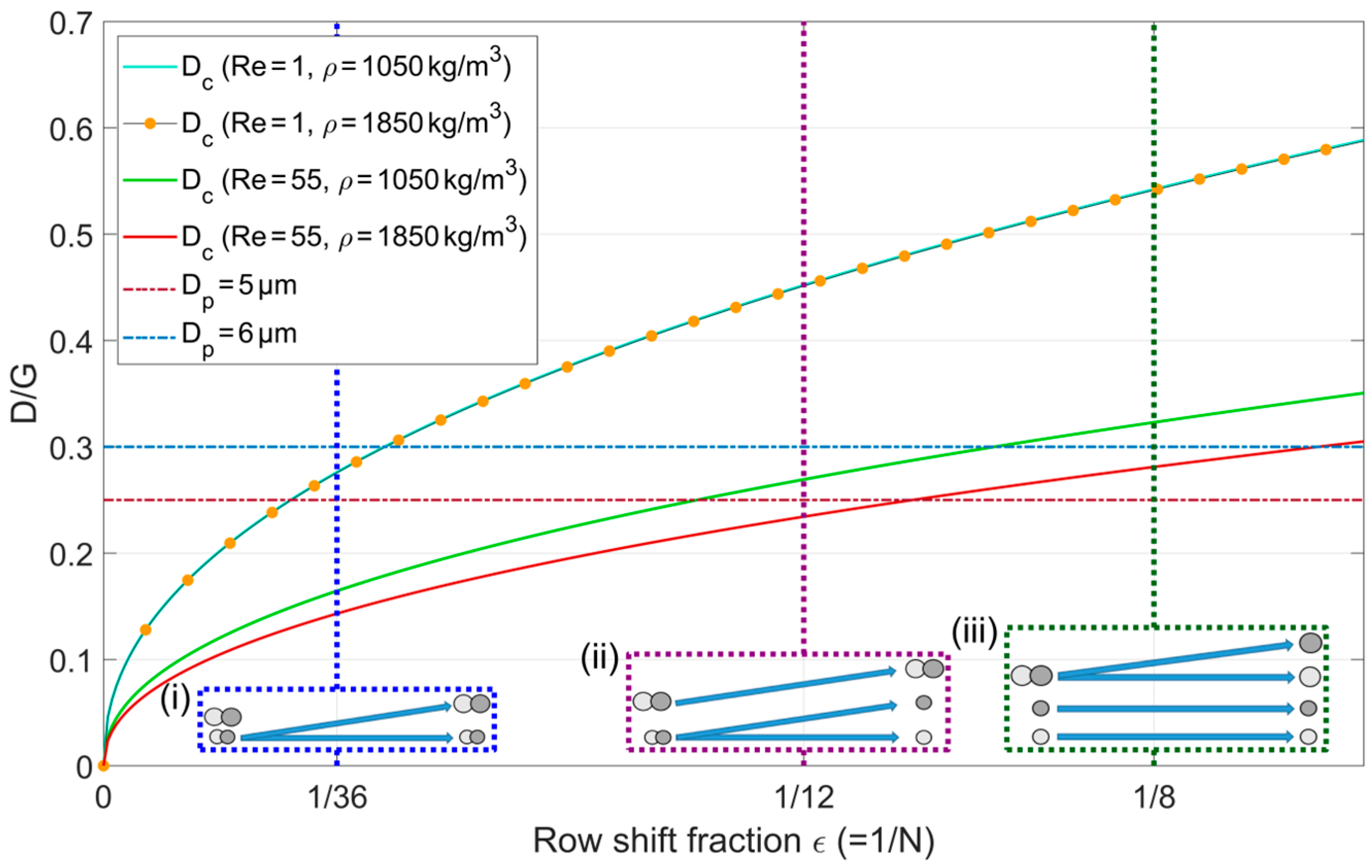
• Re = 55 (critical diameters in green and red in Figure 8); $ϵ$ = 1/12 (purple dotted vertical line in Figure 8): At this operating point the larger particles lie above their critical diameters irrespective of their density, so they continue their bump mode. For the smaller particles however, only the denser particles lie above their critical diameter whilst the lighter particles lie below theirs, meaning that the two fractions are split;
• Re = 55 (critical diameters in green and red in Figure 8); $ϵ$ = 1/8 (dark green dotted vertical line in Figure 8): At this operating point the smaller particles lie below their critical diameters and thus continue in/switch to zigzag mode. For the large particles, the denser particles lie above their critical diameter and thus show a bump mode whilst the lighter particles lie below their critical diameter which is why they show a zigzag mode.

Two things have to be noted here: Firstly whilst the switch in row shift fractions in a single channel has been done before (see e.g., [53]) and is relatively easy to realize, a change in Reynolds number is a tad more challenging. It might be realized through a change in channel depth or width. The former has the advantage that the lateral particle positions would not change but might be hard to fabricate and the latter, which might be easier to fabricate, would require measures to prevent lateral mixing of the particles as for example designated guiding structures. Secondly, even though the multidimensional fractionation into size and density is done in one step here to demonstrate its feasibility, it might be simpler to realize the fractionation in three steps, using single channels with single operating points.

To sum up, the used LBM-DEM methodology allowed not only to reproduce experimental results but was able to deliver important new results on the behavior of denser particles at elevated Reynolds numbers which would have been hard to observe experimentally.

4.2. Square Wave Serpentine Channel

The first step when investigating serpentine channels was comparing the numerical and experimental results among each other and with results from literature. The experimental data was taken in the 27th upper loop serpentine of the channel (see [10] for details on the geometry) and the numerical data of the 27th and 28th run through the numerical system (equaling one periodic element of the serpentine channel geometry, see [3] for details). Previous studies reported cases where equilibria were reached after only 3 (see [59]) or 10 (see [63]) periodic elements of the respective channels. It is thus assumed that at the investigated positions in the channels, all particles have assumed their respective equilibrium trajectories and the differences in startup between numerical and experimental systems (see [3,10]) do not matter anymore.

The comparison of numerical and experimental data was done through the juxtaposition of results of long-exposure fluorescence microscopy measurements (shown in grey in Figure 9) and numerical data of simulated particle trajectories (shown as blue lines in Figure 9). Additionally shown are the protruding ribs of the channel (blue rectangular areas in Figure 9, exemplarily labeled as R in Figure 9a. The fact that they match the ribs in the experimental data demonstrates not only the identity of the investigated channel geometries but also the perfect juxtaposition.

It can be seen that numerical and experimental data matches well in top view. To additionally ensure the identity of numerical and experimental data over channel height, APTV measurements were done and compared to numerical data for particle positions in z. The comparison showed excellent agreement (see [3]), thus validating the APTV measurements as well as the results of the numerical investigations.

The results (numerical (see [3]), as well as experimental (see [30])) furthermore agree with results from literature: At low Reynolds numbers, particles exhibit two main equilibrium streaks over channel width, which can at some point merge together into one (see e.g., [4,59,60,70]). This one streak then either persists over the whole investigated Re-range (see e.g., [4]) or defocuses again (see e.g., [4,70,71]). The transition from two into one streak happens at lower Reynolds numbers for larger particles (see e.g., [4,59,61,70]) and smaller particles are more prone to defocusing or forming multiple streaks at elevated Reynolds numbers (see. e.g., [4,59,60]).

In a next step, and to evaluate the capability of square wave serpentine channels for combined fractionation for particle size and -density, the behavior of particles of different sizes and densities was investigated (see [3,10,30]). Different to many other investigations (see e.g., [60,63]) we did not from the beginning put special focus on sections oriented along the main flow direction (see [3,30]) which (see Figure 9a) for example) will in the following be titled as horizontal channel sections. The usage of horizontal sections is intuitive, as it goes along with the linear structure of the channels. It does however not necessarily depict all occurring effects which can be exploited. Therefore we expanded our investigations to channel corner sections (see [3]) and sections orthogonal to the main flow direction (see [3,30]), which (see Figure 9a) for example) will in the following be titled as vertical channel sections.

As an analysis of z-positions of particles of different sizes and densities over the different sections and Reynolds numbers would have gone beyond the scope of our investigations, we focused on the top view here. Numbers of equilibrium streaks stated in the following therefore refer to top view only. It has however to be noted that particles of the investigated sizes and densities did not show significant sinking even though gravity was included in the simulations [3]. The reason for this is assumed to be the fact that the drag forces of the Dean vortices upstream are significantly larger than the effect of sedimentation.

Experimental (see [10,30]) and numerical investigations (see [3]) showed only minor deviations from each other. In the following only numerical results are shown, as the greater flexibility in particle parameters allowed to work with higher densities, which led to data better showing the respective effects. The corner sections did not show significant advantages to straight channel sections (see [3]). Furthermore extracting particle streaks out of a channel corner section without causing disturbance is expected to be significantly more challenging than an extraction out of a straight channel section. The following evaluations therefore focus on the straight channel sections.

Shown in Figure 10 are artificially generated intensity profiles (see [3] for details on method) representing particle distributions over channel width in the middle of horizontal (Figure 10a,b) and vertical (Figure 10c,d) channel sections. The use of intensity profiles allows for the presentation of the data without altering it by summing up particles to streaks and neglecting outliers and thus has certain advantages over the mode of presentation chosen in [3]. Presented are two datasets: The first contains particles of 1050 kg/m³ and diameters 9.89 µm (blue), 6.72 µm (green) and 3.55 µm (red) and is used to demonstrate the influence of particle size in Figure 10a,c. The second contains particles of 9.89 µm and densities 1050 kg/m³ (blue), 2000 kg/m³ (magenta) and 4000 kg/m³ (orange) and is used to demonstrate the influence of particle density in Figure 10b,d.

Analysis of the data presented in Figure 10 shows the following: In the horizontal channel section, particles of different sizes all show two equilibrium streaks over channel width at low Reynolds numbers. With rising Re these merge into one, which happens earlier, the larger the particles. At elevated Reynolds number, this one streak then starts to defocus for the smaller particles. As the two streaks of all particle types are similarly positioned and the one streak is as well, the horizontal channels sections are well suited for size fractionation in Re-areas, where one particle type shows one streak over channel width and another one shows two (compare [3]).

The behavior of the 9.89 µm particles of different densities in the horizontal channel sections is very similar: They form two equilibrium streaks at low Reynolds numbers, which lie slightly closer together the denser the particles. Those then merge into one, which happens slightly earlier for denser particles and the one streak at elevated Reynolds numbers tends a bit more to the outside, the denser the particles (compare [3]).

The behavior of differently sized particles in the vertical channel sections is similar to the behavior in horizontal sections but differs in the elevated Re-range: Here the one equilibrium streak either moves towards the downstream wall (9.89 µm, 6.72 µm) or a second streak near the downstream wall forms, whilst the original one gets weaker with rising Reynolds number (3.55 µm). The formed streaks tend to overlap, at low and elevated Reynolds numbers, but are relatively separated for example at Re = 170, which might be used for fractionation (compare [3]).

The behavior of the 9.89 µm particles of different densities in the vertical channel sections strongly resembles their behavior in horizontal channel sections with one great difference: For the investigated densities, the one streak developing at elevated Re tends strongly towards the downstream wall, the lighter the particles. This effect seems strong enough to be exploited for density fractionation (compare [3]). It is assumed to stem from lighter particles focusing closer to the channel center over height (exemplarily described in [3]), which might result in higher velocities and thus higher centrifugal forces driving particles outwards in the curves.

To sum up, the square wave serpentine microchannel is not just suited for size fractionation (see e.g., [4,10]) but can also be used for density fractionation (see also [3]). The influence of particle density can greatly differ between horizontal and vertical channel sections and based on our results, the vertical sections seem to be suited for density fractionation of larger particles (compare [3,30]). This was shown numerically (see [3]) as well as experimentally (see [30]), and can therefore be seen as validated.

4.3. Multi-Orifice Flow Fractionation Channel

To ensure functionality and to be able to compare results with literature, we use a channel with compartments identical to the ones used by Fan et al. [5] in his sharp corner MOFF channel. Specifically, each compartment is characterized by an average inlet width of 42.5 µm, followed by an 80 µm long sharp corner structure. The subsequent expansion area is designed with dimensions of 200 µm in both length and width, with an overall height of 50 µm. Due to length limitations on our chip, the channel is produced with 74 compartments before a 180° turnaround and 108 compartments afterwards (see Figure 1).

Long-exposure measurements are conducted to visualize equilibrium streaks of the used fluorescent polystyrene particles with diameters 3.55 µm (PS 3.55) and 9.92 µm (PS 9.92) (microParticles GmbH, PS-FluoRed series, Berlin, Germany). Note that the particle volume concentration is in the order of $\mathcal{O}$(10⁻⁴), indicating negligible particle-particle interactions. Images are recorded with an exposure time of 1 s at the respective last compartment (74th) in the first segment. Within the investigated Reynolds number range, streaks of these two particle types show only minor changes after the 60th compartment. This matches observations by Fan et al. [5], whose results show only minor differences between 50th (midstream) and 100th (downstream) compartments. Particles are therefore assumed to be on stable streaks in the 74th compartment.

To validate the channels capability for size fractionation that has been demonstrated by Fan et al. [5] we evaluated the behavior of 3.55 µm and 9.92 µm polystyrene (PS) particles over a range of Reynolds numbers. The characteristic velocity for the channel Reynolds number is here (following [12]) chosen to be the maximum fluid velocity. For the characteristic length, we choose the hydraulic diameter at the narrowest channel section. Wibel [72] investigated the ratio of maximum to mean flow velocity in square microchannels and found a value of 2.1 for a channel aspect ratio of 1 and 1.99 for a channel aspect ratio of two. Based on these results and taking into account the aspect ratio of 1.1765 in the narrowest section of the used channel geometry, a value of two times the averaged bulk velocity is taken for the maximum velocity in the gap.

It shows that for example at Re = 100, the smaller particles exhibit two equilibrium streaks over channel width, whilst the larger ones show only one (see Figure 11), thus validating the channels capability for size fractionation.

Fan et al. [5] states that the geometry they introduced (and we adapted) induces larger streamline curvature and thus larger centrifugal forces in the contraction area than the classic square compartment geometry. Those greater centrifugal forces then can drive larger particles to the channel centerline whilst only weakly influencing smaller particles, which stay focused on two streaks over channel width.

Based on this, particles should be much less prone to focus on a middle streak when reversing the flow in the used MOFF channel geometry as larger vortices at the compartment inlet, combined with the gradual tapering at the outlet should lead to much smaller curvature of the streamlines. To test this hypothesis, we operated the channel at a reversed flow direction, using 9.92 µm PS particles. Additionally we numerically investigated the fluid fields (308 $\times$ 220 $\times$ 55 LBM nodes, see [3] for details on simulation method) to be able to determine the curvature of streamlines. Both experimental and numerical results are shown in Figure 12.

When operating the channel in standard flow direction at Re = 100, the 9.92 µm particles are focused to the channel centerline (see Figure 12a) and the streamlines show great curvature in the contraction area (see Figure 12b). When however reversing the flow direction, the particles form an additional two streaks on the channel sides (see Figure 12c). Furthermore the streamlines show much lower curvature in the contraction area (see Figure 12d), which indicates much lower centrifugal forces. The streak pattern observed here resembles the pattern for 7.32 µm PS particles at 160 µL/min (equaling Re = 90 following our definition) in standard flow by direction observed by Fan et al. [5]. Those too can be assumed to have been much less affected by centrifugal forces than our PS 9.92 µm particles at Re = 100 in standard flow direction. The results thus agree with and confirm Fan et al. [5] who stated centrifugal forces to be the cause for particles focusing near the channel centerline.

To check whether the device is fundamentally able to focus particles onto one middle streak when operated at reversed flow direction, experiments were done with 3.55 and 9.92 µm PS particles at elevated Reynolds numbers up to 135. The results showed that some of the larger 9.92 particles exhibit circulating behavior near the side walls. The smaller PS 3.55 particles developed defocused streak patterns at elevated Reynolds numbers.

To sum up, we operated a MOFF channel in the originally intended flow direction and against it. In the original flow direction, we were able to confirm results by Fan et al. [5] who found the device suitable for size fractionation and were able to work with significantly smaller particles than they did. When reversing the flow direction, a smaller streamline curvature was expected to lead to smaller centrifugal forces and thus to particles less prone to focus in the centerline. The latter was observed experimentally and the streamline curvature numerically thus not only confirming Fan et al.’s [5] understanding of the role of centrifugal forces but furthermore demonstrating the synergy between experimental and numerical investigative methods. An investigation of equilibrium streaks observed when operating the device with reversed flow direction showed no Reynolds number area, which would have been suited for separating 3.55 and 9.92 µm PS particles with high purities: Both particle types exhibited (for the 3.55 µm particles relatively wide) side streaks, over a wide range of Reynolds numbers. At high Reynolds numbers, both particle types showed one central streak, which was however accompanied by defocusing of the particles. The strong influence of centrifugal forces we were able to confirm however, makes the MOFF channel a promising system for fractionation by particle density, which will be discussed in our future works.

5. Conclusions

In this work we were able to demonstrate the advantages of numerical and experimental approaches, but especially their combination when investigating multidimensional fractionation in microchannels. A combination of the two is extremely attractive because their respective disadvantages (e.g., need for assumptions and validation in numerical investigation or availability of data and limited choice of material parameters in experimental investigations) cancel out.

In Deterministic Lateral Displacement channels as well as in serpentine channels, we were able to show the capability for a one-step microparticle fractionation based on multiple particle properties, specifically particle size and density. Multi-Orifice Flow Fractionation channels are still subject of our current research. As however numerical and experimental results both indicate a significant influence of centrifugal forces we expect a fractionation for particle size and density to be possible.

References

- Reinecke, S.; Blahout, S.; Rosemann, T.; Kravets, B.; Wullenweber, M.; Kwade, A.; Hussong, J.; Kruggel-Emden, H. DEM-LBM simulation of multidimensional fractionation by size and density through deterministic lateral displacement at various Reynolds numbers. Powder Technol. 2021, 385, 418–433. [Google Scholar] [CrossRef]
- Huang, L.R.; Cox, E.C.; Austin, R.H.; Sturm, J.C. Continuous Particle Separation through Deterministic Lateral Displacement. Science 2004, 304, 987–990. [Google Scholar] [CrossRef] [PubMed]
- Reinecke, S.; Blahout, S.; Zhang, Z.; Rosemann, T.; Hussong, J.; Kruggel-Emden, H. Effects of particle size, particle density and Reynolds number on equilibrium streaks forming in a square wave serpentine microchannel: A DEM-LBM simulation study including experimental validation of the numerical framework. Powder Technol. 2023, 427, 118688. [Google Scholar] [CrossRef]
- Zhang, J.; Yan, S.; Sluyter, R.; Li, W.; Alici, G.; Nguyen, N.-T. Inertial particle separation by differential equilibrium positions in a symmetrical serpentine micro-channel. Sci. Rep. 2014, 4, 4527. [Google Scholar] [CrossRef] [PubMed]
- Fan, L.-L.; He, X.-K.; Han, Y.; Du, L.; Zhao, L.; Zhe, J. Continuous size-based separation of microparticles in a microchannel with symmetric sharp corner structures. Biomicrofluidics 2014, 8, 024108. [Google Scholar] [CrossRef]
- Krüger, T.; Holmes, D.; Coveney, P.V. Deformability-based red blood cell separation in deterministic lateral displacement devices—A simulation study. Biomicrofluidics 2014, 8, 054114. [Google Scholar] [CrossRef] [PubMed]
- Dincau, B.M.; Aghilinejad, A.; Hammersley, T.; Chen, X.; Kim, J.-H. Deterministic lateral displacement (DLD) in the high Reynolds number regime: High-throughput and dynamic separation characteristics. Microfluid. Nanofluidics 2018, 22, 59. [Google Scholar] [CrossRef]
- Aghilinejad, A.; Aghaamoo, M.; Chen, X. On the transport of particles/cells in high-throughput deterministic lateral displacement devices: Implications for circulating tumor cell separation. Biomicrofluidics 2019, 13, 034112. [Google Scholar] [CrossRef]
- Inglis, D.W.; Davis, J.A.; Austin, R.H.; Sturm, J.C. Critical particle size for fractionation by deterministic lateral displacement. Lab Chip 2006, 6, 655–658. [Google Scholar] [CrossRef]
- Blahout, S.; Reinecke, S.R.; Kazerooni, H.T.; Kruggel-Emden, H.; Hussong, J. On the 3D distribution and size fractionation of microparticles in a serpentine microchannel. Microfluid. Nanofluidics 2020, 24, 22. [Google Scholar] [CrossRef]
- Zhang, J.; Li, W.; Li, M.; Alici, G.; Nguyen, N.-T. Particle inertial focusing and its mechanism in a serpentine microchannel. Microfluid. Nanofluidics 2014, 17, 305–316. [Google Scholar] [CrossRef]
- Park, J.-S.; Jung, H.-I. Multiorifice Flow Fractionation: Continuous Size-Based Separation of Microspheres Using a Series of Contraction/Expansion Microchannels. Anal. Chem. 2009, 81, 8280–8288. [Google Scholar] [CrossRef] [PubMed]
- Bußmann, S.; Kruggel-Emden, H.; Reichert, M. Realizing fragment spawning and fragment growth in the parallelized Discrete Element Method (DEM) during modelling of comminution. Adv. Powder Technol. 2021, 32, 2171–2191. [Google Scholar] [CrossRef]
- Oschmann, T.; Hold, J.; Kruggel-Emden, H. Numerical investigation of mixing and orientation of non-spherical particles in a model type fluidized bed. Powder Technol. 2014, 258, 304–323. [Google Scholar] [CrossRef]
- Bauer, A.; Maier, G.; Reith-Braun, M.; Kruggel-Emden, H.; Pfaff, F.; Gruna, R.; Hanebeck, U.; Längle, T. Towards a feed material adaptive optical belt sorter: A simulation study utilizing a DEM-CFD approach. Powder Technol. 2022, 411, 117917. [Google Scholar] [CrossRef]
- Schulz, D.; Reinecke, S.R.; Woschny, N.; Schmidt, E.; Kruggel-Emden, H. Development and evaluation of force balance based functions for dust detachment from bulk particles stressed by fluid flow. Powder Technol. 2023, 417, 118257. [Google Scholar] [CrossRef]
- Kolck, V.; Witte, J.; Schmidt, E.; Kruggel-Emden, H. Analysis of process parameter sensitivities of jet-based direct mixing gas phase hetero-agglomeration by DEM/CFD-modelling. Powder Technol. 2023, 429, 118963. [Google Scholar] [CrossRef]
- Rosemann, T.; Kravets, B.; Reinecke, S.; Kruggel-Emden, H.; Wu, M.; Peters, B. Comparison of numerical schemes for 3D lattice Boltzmann simulations of moving rigid particles in thermal fluid flows. Powder Technol. 2019, 356, 528–546. [Google Scholar] [CrossRef]
- Kravets, B.; Schulz, D.; Jasevičius, R.; Reinecke, S.; Rosemann, T.; Kruggel-Emden, H. Comparison of particle-resolved DNS (PR-DNS) and non-resolved DEM/CFD simulations of flow through homogenous ensembles of fixed spherical and non-spherical particles. Adv. Powder Technol. 2021, 32, 1170–1195. [Google Scholar] [CrossRef]
- Rosemann, T.; Reinecke, S.R.; Kruggel-Emden, H. Analysis of Mobility Effects in Particle-Gas Flows by Particle-Resolved LBM-DEM Simulations. Chem. Ing. Tech. 2021, 93, 223–236. [Google Scholar] [CrossRef]
- Kruggel-Emden, H.; Kravets, B.; Suryanarayana, M.; Jasevicius, R. Direct numerical simulation of coupled fluid flow and heat transfer for single particles and particle packings by a LBM-approach. Powder Technol. 2016, 294, 236–251. [Google Scholar] [CrossRef]
- Kravets, B.; Rosemann, T.; Reinecke, S.; Kruggel-Emden, H. A new drag force and heat transfer correlation derived from direct numerical LBM-simulations of flown through particle packings. Powder Technol. 2019, 345, 438–456. [Google Scholar] [CrossRef]
- Aidun, C.K.; Clausen, J.R. Lattice-Boltzmann Method for Complex Flows. Annu. Rev. Fluid Mech. 2010, 42, 439–472. [Google Scholar] [CrossRef]
- McNamara, G.R.; Zanetti, G. Use of the Boltzmann Equation to Simulate Lattice-Gas Automata. Phys. Rev. Lett. 1988, 61, 2332–2335. [Google Scholar] [CrossRef] [PubMed]
- Bouzidi, M.; Firdaouss, M.; Lallemand, P. Momentum transfer of a Boltzmann-lattice fluid with boundaries. Phys. Fluids 2001, 13, 3452–3459. [Google Scholar] [CrossRef]
- Peng, C.; Ayala, O.M.; Wang, L.-P. A comparative study of immersed boundary method and interpolated bounce-back scheme for no-slip boundary treatment in the lattice Boltzmann method: Part I, laminar flows. Comput. Fluids 2019, 192, 104233. [Google Scholar] [CrossRef]
- Tao, S.; Hu, J.; Guo, Z. An investigation on momentum exchange methods and refilling algorithms for lattice Boltzmann simulation of particulate flows. Comput. Fluids 2016, 133, 1–14. [Google Scholar] [CrossRef]
- Guo, Y.; Curtis, J.S. Discrete Element Method Simulations for Complex Granular Flows. Annu. Rev. Fluid Mech. 2015, 47, 21–46. [Google Scholar] [CrossRef]
- Shan, X. Simulation of Rayleigh-Bénard convection using a lattice Boltzmann method. Phys. Rev. E 1997, 55, 2780–2788. [Google Scholar] [CrossRef]
- Blahout, S. On the Multi-Dimensional Microparticle Fractionation in a Sharp-Corner Serpentine Microchannel—An Experimental and Numerical Study. Ph.D. Thesis, TU Darmstadt, Darmstadt, Germany, 2022. [Google Scholar]
- Cierpka, C.; Kähler, C.J. Particle imaging techniques for volumetric three-component (3D3C) velocity measurements in microfluidics. J. Vis. 2012, 15, 1–31. [Google Scholar] [CrossRef]
- Cierpka, C.; Rossi, M.; Segura, R.; Kähler, C.J. On the calibration of astigmatism particle tracking velocimetry for microflows. Meas. Sci. Technol. 2011, 22, 015401. [Google Scholar] [CrossRef]
- Kao, H.; Verkman, A. Tracking of single fluorescent particles in three dimensions: Use of cylindrical optics to encode particle position. Biophys. J. 1994, 67, 1291–1300. [Google Scholar] [CrossRef]
- Santiago, J.G.; Wereley, S.T.; Meinhart, C.D.; Beebe, D.J.; Adrian, R.J. A particle image velocimetry system for microfluidics. Exp. Fluids 1998, 25, 316–319. [Google Scholar] [CrossRef]
- Westerweel, J.; Geelhoed, P.F.; Lindken, R. Single-pixel resolution ensemble correlation for micro-PIV applications. Exp. Fluids 2004, 37, 375–384. [Google Scholar] [CrossRef]
- Lindken, R.; Rossi, M.; Große, S.; Westerweel, J. Micro-Particle Image Velocimetry (µPIV): Recent developments, applications, and guidelines. Lab Chip 2009, 9, 2551–2567. [Google Scholar] [CrossRef] [PubMed]
- Westerweel, J. Fundamentals of digital particle image velocimetry. Meas. Sci. Technol. 1997, 8, 1379–1392. [Google Scholar] [CrossRef]
- Adrian, R.J. Particle-Imaging Techniques for Experimental Fluid Mechanics. Annu. Rev. Fluid Mech. 1991, 23, 261–304. [Google Scholar] [CrossRef]
- Keane, R.D.; Adrian, R.J. Theory of cross-correlation analysis of PIV images. Appl. Sci. Res. 1992, 49, 191–215. [Google Scholar] [CrossRef] [PubMed]
- Olsen, M.G.; Adrian, R.J. Out-of-focus effects on particle image visibility and correlation in microscopic particle image velocimetry. Exp. Fluids 2000, 29, S166–S174. [Google Scholar] [CrossRef]
- Wereley, S.T.; Gui, L.; Meinhart, C.D. Advanced Algorithms for Microscale Particle Image Velocimetry. AIAA J. 2002, 40, 1047–1055. [Google Scholar] [CrossRef]
- Keane, R.D.; Adrian, R.J. Optimization of particle image velocimeters. I. Double pulsed systems. Meas. Sci. Technol. 1990, 1, 1202–1215. [Google Scholar] [CrossRef]
- Meinhart, C.D.; Wereley, S.T.; Santiago, J.G. A PIV Algorithm for Estimating Time-Averaged Velocity Fields. J. Fluids Eng. 2000, 122, 285–289. [Google Scholar] [CrossRef]
- McGrath, J.; Jimenez, M.; Bridle, H. Deterministic lateral displacement for particle separation: A review. Lab Chip 2014, 14, 4139–4158. [Google Scholar] [CrossRef] [PubMed]
- Sim, T.S.; Kwon, K.; Park, J.C.; Lee, J.-G.; Jung, H.-I. Multistage-multiorifice flow fractionation (MS-MOFF): Continuous size-based separation of microspheres using multiple series of contraction/expansion microchannels. Lab Chip 2011, 11, 93–99. [Google Scholar] [CrossRef]
- Park, J.-S.; Song, S.-H.; Jung, H.-I. Continuous focusing of microparticles using inertial lift force and vorticity via multi-orifice microfluidic channels. Lab Chip 2009, 9, 939–948. [Google Scholar] [CrossRef] [PubMed]
- Zeming, K.K.; Salafi, T.; Chen, C.-H.; Zhang, Y. Asymmetrical Deterministic Lateral Displacement Gaps for Dual Functions of Enhanced Separation and Throughput of Red Blood Cells. Sci. Rep. 2016, 6, 22934. [Google Scholar] [CrossRef] [PubMed]
- Vernekar, R.; Krüger, T.; Loutherback, K.; Morton, K.; Inglis, D.W. Anisotropic permeability in deterministic lateral displacement arrays. Lab Chip 2017, 17, 3318–3330. [Google Scholar] [CrossRef] [PubMed]
- Kulrattanarak, T.; van der Sman, R.; Lubbersen, Y.; Schroën, C.; Pham, H.; Sarro, P.; Boom, R. Mixed motion in deterministic ratchets due to anisotropic permeability. J. Colloid Interface Sci. 2011, 354, 7–14. [Google Scholar] [CrossRef] [PubMed]
- Wullenweber, M.S.; Kottmeier, J.; Kampen, I.; Dietzel, A.; Kwade, A. Simulative Investigation of Different DLD Microsystem Designs with Increased Reynolds Numbers Using a Two-Way Coupled IBM-CFD/6-DOF Approach. Processes 2022, 10, 403. [Google Scholar] [CrossRef]
- Loutherback, K.; D’Silva, J.; Liu, L.; Wu, A.; Austin, R.H.; Sturm, J.C. Deterministic separation of cancer cells from blood at 10 mL/min. AIP Adv. 2012, 2, 042107. [Google Scholar] [CrossRef]
- Kulrattanarak, T.; van der Sman, R.G.M.; Schroën, C.G.P.H.; Boom, R.M. Analysis of mixed motion in deterministic ratchets via experiment and particle simulation. Microfluid. Nanofluidics 2011, 10, 843–853. [Google Scholar] [CrossRef]
- Davis, J.A. Microfluidic Separation of Blood Components through Deterministic Lateral Displacement. Ph.D. Thesis, Princeton University, Princeton, NJ, USA, 2008. [Google Scholar]
- Kottmeier, J.; Wullenweber, M.; Blahout, S.; Hussong, J.; Kampen, I.; Kwade, A.; Dietzel, A. Accelerated Particle Separation in a DLD Device at Re > 1 Investigated by Means of µPIV. Micromachines 2019, 10, 768. [Google Scholar] [CrossRef] [PubMed]
- Lubbersen, Y.; Dijkshoorn, J.; Schutyser, M.; Boom, R. Visualization of inertial flow in deterministic ratchets. Sep. Purif. Technol. 2013, 109, 33–39. [Google Scholar] [CrossRef]
- Di Carlo, D.; Irimia, D.; Tompkins, R.G.; Toner, M. Continuous inertial focusing, ordering, and separation of particles in microchannels. Proc. Natl. Acad. Sci. USA 2007, 104, 18892–18897. [Google Scholar] [CrossRef] [PubMed]
- Martel, J.M.; Toner, M. Inertial Focusing in Microfluidics. Annu. Rev. Biomed. Eng. 2014, 16, 371–396. [Google Scholar] [CrossRef] [PubMed]
- Di Carlo, D. Inertial microfluidics. Lab Chip 2009, 9, 3038–3046. [Google Scholar] [CrossRef] [PubMed]
- Ying, Y.; Lin, Y. Inertial Focusing and Separation of Particles in Similar Curved Channels. Sci. Rep. 2019, 9, 16575. [Google Scholar] [CrossRef]
- Jiang, D.; Tang, W.; Xiang, N.; Ni, Z. Numerical simulation of particle focusing in a symmetrical serpentine microchannel. RSC Adv. 2016, 6, 57647–57657. [Google Scholar] [CrossRef]
- Bazaz, S.R.; Mihandust, A.; Salomon, R.; Joushani, H.A.N.; Li, W.; Amiri, H.A.; Mirakhorli, F.; Zhand, S.; Shrestha, J.; Miansari, M.; et al. Zigzag microchannel for rigid inertial separation and enrichment (Z-RISE) of cells and particles. Lab Chip 2022, 22, 4093–4109. [Google Scholar] [CrossRef] [PubMed]
- Wang, L.; Dandy, D.S. High-Throughput Inertial Focusing of Micrometer- and Sub-Micrometer-Sized Particles Separation. Adv. Sci. 2017, 4, 1700153. [Google Scholar] [CrossRef] [PubMed]
- Zhang, J.; Yan, S.; Li, W.; Alici, G.; Nguyen, N.-T. High throughput extraction of plasma using a secondary flow-aided inertial microfluidic device. RSC Adv. 2014, 4, 33149–33159. [Google Scholar] [CrossRef]
- Yuan, D.; Sluyter, R.; Zhao, Q.; Tang, S.; Yan, S.; Yun, G.; Li, M.; Zhang, J.; Li, W. Dean-flow-coupled elasto-inertial particle and cell focusing in symmetric serpentine microchannels. Microfluid. Nanofluidics 2019, 23, 41. [Google Scholar] [CrossRef]
- Rodriguez-Mateos, P.; Ngamsom, B.; Dyer, C.E.; Iles, A.; Pamme, N. Inertial focusing of microparticles, bacteria, and blood in serpentine glass channels. Electrophoresis 2021, 42, 2246–2255. [Google Scholar] [CrossRef] [PubMed]
- Moon, H.-S.; Kwon, K.; Kim, S.-I.; Han, H.; Sohn, J.; Lee, S.; Jung, H.-I. Continuous separation of breast cancer cells from blood samples using multi-orifice flow fractionation (MOFF) and dielectrophoresis (DEP). Lab Chip 2011, 11, 1118–1125. [Google Scholar] [CrossRef]
- Beech, J.P. Microfluidics Separation and Analysis of Biological Particles. Ph.D. Thesis, Lund University, Lund, Sweden, 2011. [Google Scholar]
- Imad, A.; Ouâkka, A.; Van, K.D.; Mesmacque, G. Analysis of the Viscoelastoplastic Behavior of Expanded Polystyrene under Compressive Loading: Experiments and Modeling. Strength Mater. 2001, 33, 140–149. [Google Scholar] [CrossRef]
- Rodriguez, V.; Saurel, R.; Jourdan, G.; Houas, L. Solid-particle jet formation under shock-wave acceleration. Phys. Rev. E 2013, 88, 063011. [Google Scholar] [CrossRef] [PubMed]
- Cha, H.; Fallahi, H.; Dai, Y.; Yadav, S.; Hettiarachchi, S.; McNamee, A.; An, H.; Xiang, N.; Nguyen, N.-T.; Zhang, J. Tuning particle inertial separation in sinusoidal channels by embedding periodic obstacle microstructures. Lab Chip 2022, 22, 2789–2800. [Google Scholar] [CrossRef] [PubMed]
- Zhang, J.; Yuan, D.; Zhao, Q.; Teo, A.J.T.; Yan, S.; Ooi, C.H.; Li, W.; Nguyen, N.-T. Fundamentals of Differential Particle Inertial Focusing in Symmetric Sinusoidal Microchannels. Anal. Chem. 2019, 91, 4077–4084. [Google Scholar] [CrossRef] [PubMed]
- Wibel, W. Untersuchung zu Laminarer, Transitioneller und Turbulenter Strömung in Rechteckigen Mikrokanälen. Ph.D. Thesis, Technischen Universität Dortmund, Dortmund, Germany, 2008. [Google Scholar]
Disclaimer/Publisher’s Note: The statements, opinions and data contained in all publications are solely those of the individual author(s) and contributor(s) and not of MDPI and/or the editor(s). MDPI and/or the editor(s) disclaim responsibility for any injury to people or property resulting from any ideas, methods, instructions or products referred to in the content. |
© 2024 by the authors. Licensee MDPI, Basel, Switzerland. This article is an open access article distributed under the terms and conditions of the Creative Commons Attribution (CC BY) license (https://creativecommons.org/licenses/by/4.0/).
Share and Cite
Reinecke, S.R.; Zhang, Z.; Blahout, S.; Radecki-Mundinger, E.; Hussong, J.; Kruggel-Emden, H. Investigation of Multidimensional Fractionation in Microchannels Combining a Numerical DEM-LBM Approach with Optical Measurements. Powders 2024, 3, 305-323. https://doi.org/10.3390/powders3020018
Reinecke SR, Zhang Z, Blahout S, Radecki-Mundinger E, Hussong J, Kruggel-Emden H. Investigation of Multidimensional Fractionation in Microchannels Combining a Numerical DEM-LBM Approach with Optical Measurements. Powders. 2024; 3(2):305-323. https://doi.org/10.3390/powders3020018
Chicago/Turabian StyleReinecke, Simon Raoul, Zihao Zhang, Sebastian Blahout, Edgar Radecki-Mundinger, Jeanette Hussong, and Harald Kruggel-Emden. 2024. "Investigation of Multidimensional Fractionation in Microchannels Combining a Numerical DEM-LBM Approach with Optical Measurements" Powders 3, no. 2: 305-323. https://doi.org/10.3390/powders3020018
APA StyleReinecke, S. R., Zhang, Z., Blahout, S., Radecki-Mundinger, E., Hussong, J., & Kruggel-Emden, H. (2024). Investigation of Multidimensional Fractionation in Microchannels Combining a Numerical DEM-LBM Approach with Optical Measurements. Powders, 3(2), 305-323. https://doi.org/10.3390/powders3020018