
Comparative Analysis of Linear Models and Artificial Neural Networks for Sugar Price Prediction

 , , , , ,
  , and
, and 
Abstract
:1. Introduction
2. Materials and Methods
2.1. Autoregressive Model (AR)
2.2. Autoregressive Moving and Average Model (ARMA)
2.3. Multilayer Perceptron (MLP)
2.4. Extreme Learning Machine (ELM)
2.5. Elman and Jordan Networks
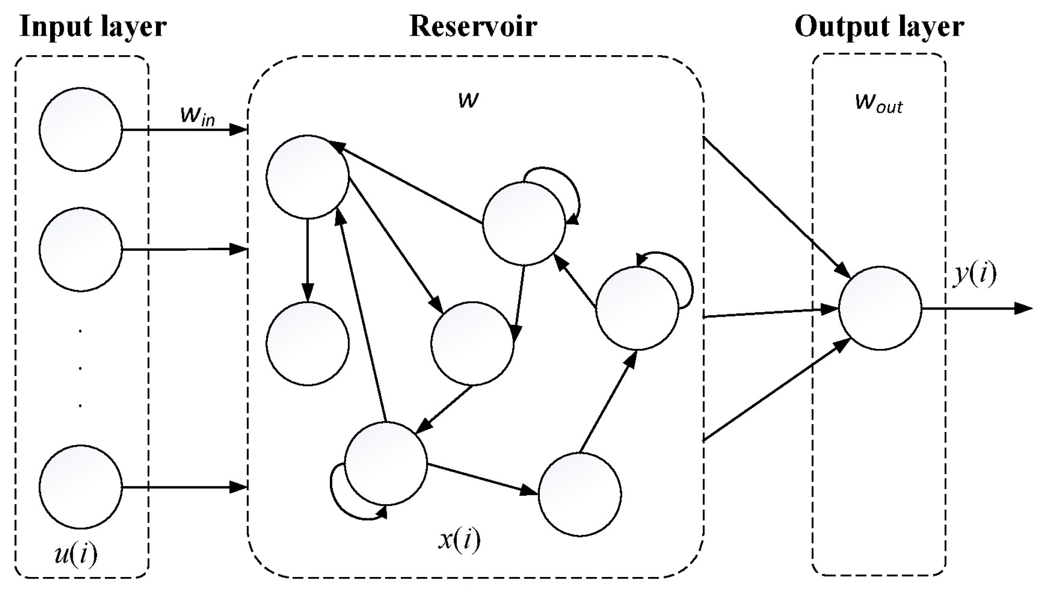
2.6. Echo State Network (ESN)
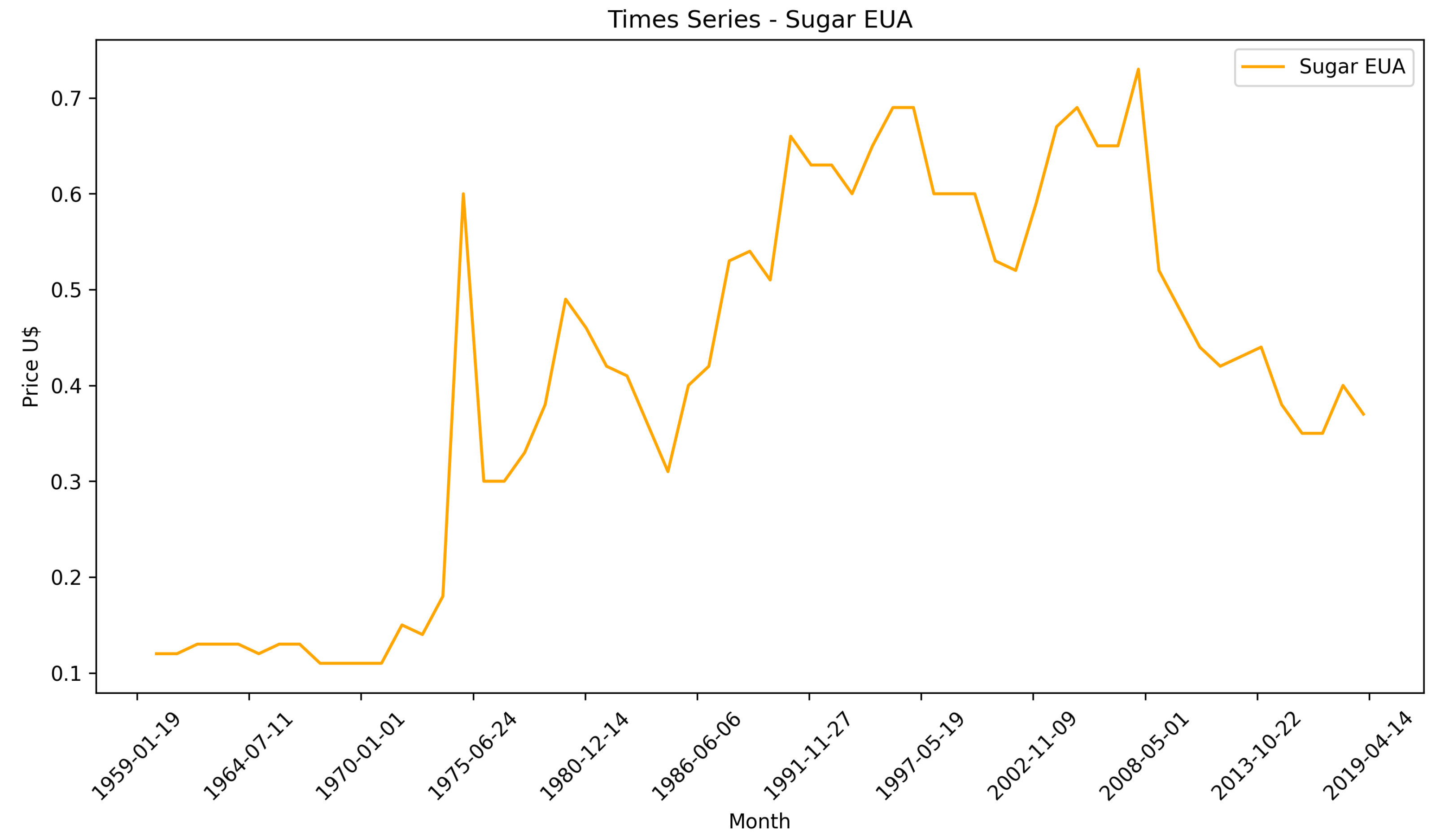
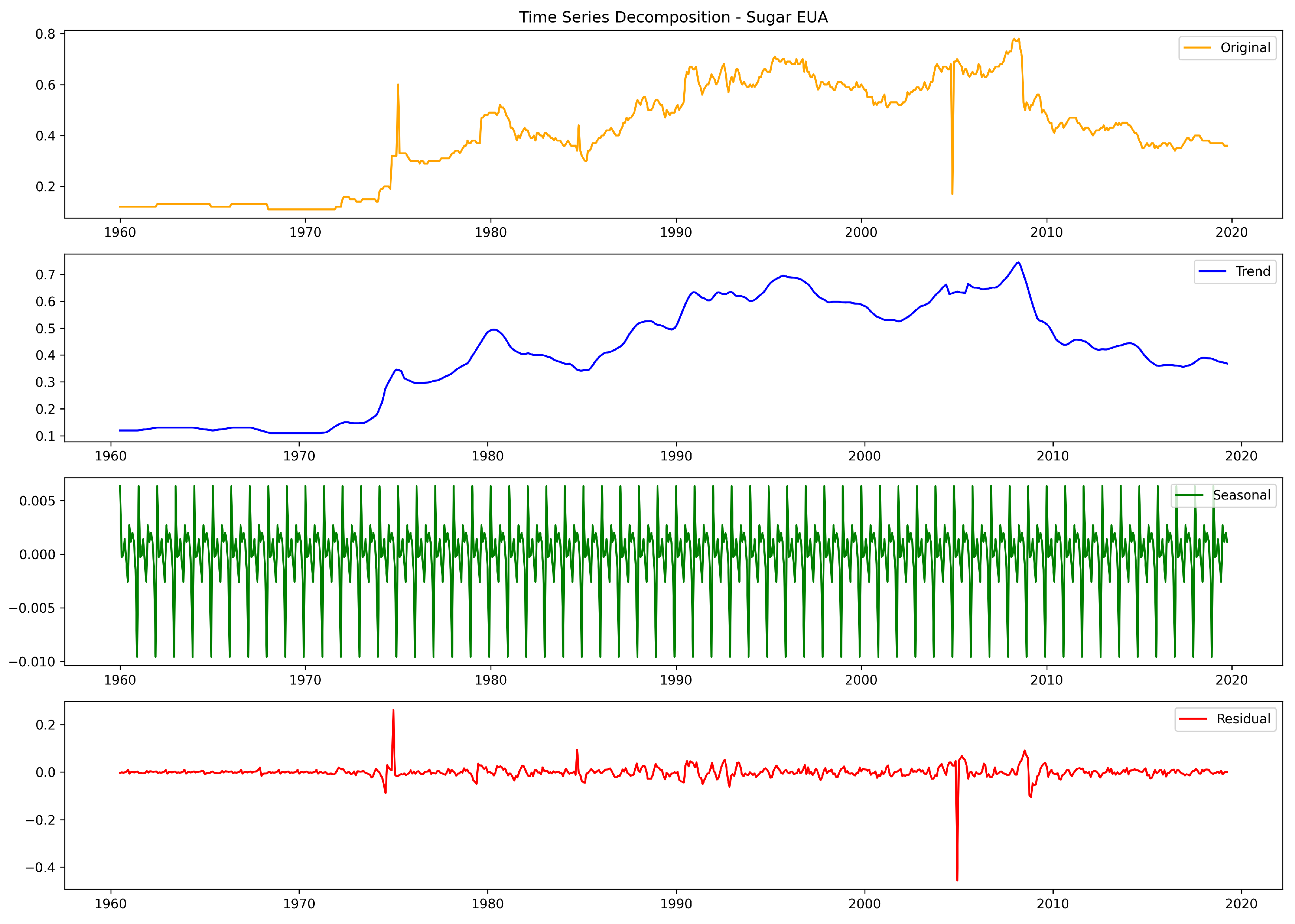
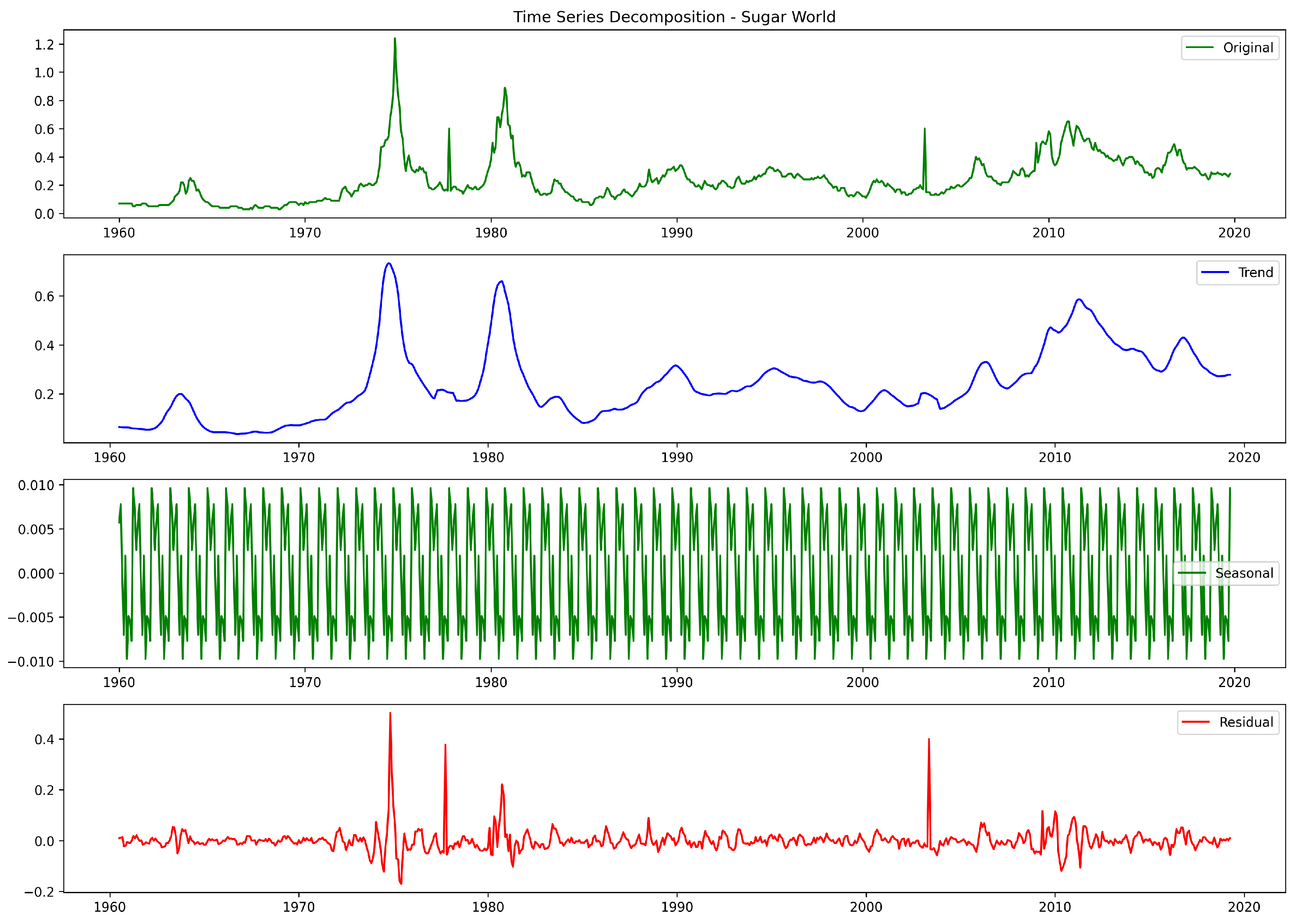
3. Data Analysis and Processing
Performance Assessment
4. Results and Discussion
5. Conclusions
Author Contributions
Funding
Institutional Review Board Statement
Informed Consent Statement
Data Availability Statement
Conflicts of Interest
References
- OECD-FAO. OECD-FAO Agricultural Outlook 2019. 2023. Available online: https://www.oecd.org/agriculture/oecd-fao-agricultural-outlook-2019/ (accessed on 1 March 2021).
- Salehi, R.; Asaadi, M.A.; Rahimi, M.H.; Mehrabi, A. The information technology barriers in supply chain of sugarcane in Khuzestan province, Iran: A combined ANP-DEMATEL approach. Inf. Process. Agric. 2021, 8, 458–468. [Google Scholar] [CrossRef]
- Silva, N.; Siqueira, I.; Okida, S.; Stevan, S.L.; Siqueira, H. Neural Networks for Predicting Prices of Sugarcane Derivatives. Sugar Tech 2019, 21, 514–523. [Google Scholar] [CrossRef]
- Deina, C.; Prates, M.H.d.A.; Alves, C.H.R.; Martins, M.S.R.; Trojan, F.; Stevan, S.L., Jr.; Siqueira, H.V. A methodology for coffee price forecasting based on extreme learning machines. Inf. Process. Agric. 2022, 9, 556–565. [Google Scholar] [CrossRef]
- Maitah, M.; Smutka, L. The Development of World Sugar Prices. Sugar Tech 2019, 21, 1–8. [Google Scholar] [CrossRef]
- der Mensbrugghe, D.V.; Beghin, J.C.; Mitchell, D. Modeling Tariff Rate Quotas in a Global Context: The Case of Sugar Markets in OECD Countries; Food and Agricultural Policy Research Institute (FAPRI): Ames, IA, USA, 2003. [Google Scholar]
- OECD and Food and Agriculture Organization of the United Nations. OECD-FAO Agricultural Outlook 2016–2025; OECD: Paris, France, 2016; 136p. [Google Scholar] [CrossRef]
- Rumánková, L.; Smutka, L.; Maitah, M.; Benešová, I. The Interrelationship between Sugar Prices at the Main World Sugar Commodities Markets. Sugar Tech 2019, 21, 853–861. [Google Scholar] [CrossRef]
- Van der Eng, P. Agricultural Growth in Indonesia: Productivity Change and Policy Impact since 1880; Springer: London, UK, 1996. [Google Scholar]
- Yara Brasil. Produção Mundial de Cana-de-Açúcar. Available online: https://www.yarabrasil.com.br/conteudo-agronomico/blog/producao-mundial-de-cana-de-acucar/ (accessed on 1 March 2021).
- OECD and Food and Agriculture Organization of the United Nations. OECD-FAO Agricultural Outlook 2019–2028; OECD: Paris, France, 2019; 326p, Available online: https://www.oecd-ilibrary.org/content/publication/agr_outlook-2019-en (accessed on 1 March 2021).
- USDA; FAS. Sugar: World Markets and Trade. 2020. Available online: https://fas.usda.gov/data/sugar-world-markets-and-trade (accessed on 1 March 2021).
- Lin, B.; Variyam, J.N.; Allshouse, J.E.; Cromartie, J. Food and Agricultural Commodity Consumption in the United States: Looking Ahead To 2020; Agricultural Economic Reports, Number 33959; United States Department of Agriculture, Economic Research Service: Washington, DC, USA, 2003; Available online: https://ideas.repec.org/p/ags/uerser/33959.html (accessed on 1 March 2021).
- Pagani, V.; Stella, T.; Guarneri, T.; Finotto, G.; Berg, M.v.; Marin, F.R.; Acutis, M.; Confalonieri, R. Forecasting sugarcane yields using agro-climatic indicators and Canegro model: A case study in the main production region in Brazil. Agric. Syst. 2017, 154, 45–52. [Google Scholar] [CrossRef]
- Amrouk, E.M.; Heckelei, T. Forecasting International Sugar Prices: A Bayesian Model Average Analysis. Sugar Tech 2020, 22, 552–562. [Google Scholar] [CrossRef]
- Adenäuer, M.; Louhichi, K.; de Frahan, B.H.; Witzke, H.P. Impact of the “Everything but Arms” Initiative on the EU Sugar Sub-Sector. EcoMod2004, 2010, 330600001. Available online: https://ideas.repec.org/p/ekd/003306/330600001.html (accessed on 1 March 2021).
- Nolte, S.; Buysse, J.; Huylenbroeck, G.V. Modelling the Effects of an Abolition of the EU Sugar Quota on Internal Prices, Production, and Imports. In Proceedings of the 114th Seminar, Berlin, Germany, 15–16 April 2010; European Association of Agricultural Economists: Wageningen, The Netherlands, 2010. Available online: https://ideas.repec.org/p/ags/eaa114/61346.html (accessed on 1 March 2021).
- Stephen Haley. World Raw Sugar Prices: The Influence of Brazilian Costs of Production and World Surplus/Deficit Measures; United States Department of Agriculture: Washington, DC, USA, 2013.
- Haley, S. Projecting World Raw Sugar Prices; EMS/USDA: Washington, DC, USA, 2015.
- Chang, C.; McAleer, M.; Wang, Y. Modelling Volatility Spillovers for Bio-ethanol, Sugarcane and Corn Spot and Futures Prices. Renew. Sustain. Energy Rev. 2018, 81, 1002–1018. [Google Scholar] [CrossRef]
- Rabobank. Sugar Quarterly Q4 2020. Available online: https://research.rabobank.com/far/en/sectors/sugar/sugar-quarterly-q4-2020.html (accessed on 1 March 2021).
- Bisgaard, S.; Kulahci, M. Time Series Analysis and Forecasting by Example; John Wiley & Sons: Hoboken, NJ, USA, 2011. [Google Scholar]
- Ribeiro, C.; Oliveira, S. A Hybrid Commodity Price-Forecasting Model Applied to the Sugar–Alcohol Sector. Aust. J. Agric. Resour. Econ. 2011, 55, 180–198. [Google Scholar] [CrossRef]
- de Melo, B.; Milioni, A.Z.; Júnior, C.L.N. Daily and Monthly Sugar Price Forecasting Using the Mixture of Local Expert Models. Pesqui. Oper. 2007, 27, 235–246. [Google Scholar] [CrossRef]
- Esam, A.B. Economic Modelling and Forecasting of Sugar Production and Consumption in Egypt. Int. J. Agric. Econ. 2017, 2, 96–109. [Google Scholar] [CrossRef]
- Mehmood, Q.; Sial, M.H.; Riaz, M.; Shaheen, N. Forecasting the Production of Sugarcane in Pakistan for the Year 2018–2030, Using Box-Jenkin’s Methodology. JAPS J. Anim. Plant Sci. 2019, 29, 1396–1401. [Google Scholar]
- Vishawajith, K.P.; Sahu, P.K.; Dhekale, B.S.; Mishra, P. Modelling and Forecasting Sugarcane and Sugar Production in India. Indian J. Econ. Dev. 2016, 12, 71–80. [Google Scholar] [CrossRef]
- Box, G.E.P.; Jenkins, G.M.; Reinsel, G.C.; Ljung, G.M. Time Series Analysis: Forecasting and Control; John Wiley & Sons: Hoboken, NJ, USA, 2015. [Google Scholar]
- Santos, D.S.d., Jr.; Neto, P.S.G.d.; Oliveira, J.a.F.L.d.; Siqueira, H.V.; Barchi, T.M.; Lima, A.R.; Madeiro, F.; Dantas, D.A.P.; Converti, A.; Pereira, A.C.; et al. Solar Irradiance Forecasting Using Dynamic Ensemble Selection. Appl. Sci. 2022, 12, 3510. [Google Scholar] [CrossRef]
- Nayak, S.K.; Nayak, S.C.; Das, S. Modeling and Forecasting Cryptocurrency Closing Prices with Rao Algorithm-Based Artificial Neural Networks: A Machine Learning Approach. FinTech 2021, 1, 47–62. [Google Scholar] [CrossRef]
- Neto, P.S.G.d.; Oliveira, J.a.F.L.d.; Júnior, D.S.d.O.S.; Siqueira, H.V.; Marinho, M.H.D.N.; Madeiro, F. A Hybrid Nonlinear Combination System for Monthly Wind Speed Forecasting. IEEE Access 2020, 8, 191365–191377. [Google Scholar] [CrossRef]
- Suresh, K.K.; Priya, S.R.K. Forecasting Sugarcane Yield of Tamilnadu Using ARIMA Models. Sugar Tech 2011, 13, 23–26. [Google Scholar] [CrossRef]
- Kotu, V.; Deshpande, B. (Eds.) Chapter 12–Time Series Forecasting. In Data Science, 2nd ed.; Morgan Kaufmann: Burlington, MA, USA, 2019; pp. 395–445. ISBN 978-0-12-814761-0. [Google Scholar] [CrossRef]
- Gyamerah, S.A.; Arthur, J.; Akuamoah, S.W.; Sithole, Y. Measurement and Impact of Longevity Risk in Portfolios of Pension Annuity: The Case in Sub Saharan Africa. FinTech 2023, 2, 48–67. [Google Scholar] [CrossRef]
- Siqueira, H.; Luna, I.; Alves, T.A.; Tadano, Y.d. The Direct Connection Between Box & Jenkins Methodology and Adaptive Filtering Theory. Math. Eng. Sci. Aerosp. (MESA) 2019, 10, 27. [Google Scholar]
- Maceira, M.E.P.; Damázio, J.M. Use of the PAR (p) Model in the Stochastic Dual Dynamic Programming Optimization Scheme Used in the Operation Planning of the Brazilian Hydropower System. Probab. Eng. Inf. Sci. 2006, 20, 143–156. [Google Scholar] [CrossRef]
- Hong, Y. Hypothesis Testing in Time Series via the Empirical Characteristic Function: A Generalized Spectral Density Approach. J. Am. Stat. Assoc. 1999, 94, 1201–1220. [Google Scholar] [CrossRef]
- Kosmas, I.; Papadopoulos, T.; Dede, G.; Michalakelis, C. The Use of Artificial Neural Networks in the Public Sector. FinTech 2023, 2, 138–152. [Google Scholar] [CrossRef]
- Belotti, J.; Siqueira, H.; Araujo, L.; Stevan, S.L., Jr.; de Mattos Neto, P.S.; Marinho, M.H.N.; Oliveira, J.F.L.d.; Usberti, F.; Filho, M.d.A.L.; Converti, A.; et al. Neural-based ensembles and unorganized machines to predict streamflow series from hydroelectric plants. Energies 2020, 13, 4769. [Google Scholar] [CrossRef]
- Siqueira, H.V.; Boccato, L.; Attux, R.; Filho, C.L. Echo state networks in seasonal streamflow series prediction. Learn. Nonlinear Model. 2012, 10, 181–191. [Google Scholar] [CrossRef]
- Siqueira, H.; Boccato, L.; Attux, R.; Lyra, C. Unorganized machines for seasonal streamflow series forecasting. Int. J. Neural Syst. 2014, 24, 1430009. [Google Scholar] [CrossRef]
- Haykin, S. Neural Networks: A Comprehensive Foundation; Prentice-Hall, Inc.: Hoboken, NJ, USA, 2007. [Google Scholar]
- Siqueira, H.; Luna, I. Performance comparison of feedforward neural networks applied to streamflow series forecasting. Math. Eng. Sci. Aerosp. (MESA) 2019, 10, 41. [Google Scholar]
- Huang, G.; Zhu, Q.; Siew, C. Extreme learning machine: A new learning scheme of feedforward neural networks. In Proceedings of the 2004 IEEE International Joint Conference on Neural Networks (IEEE Cat. No.04CH37541), Budapest, Hungary, 25–29 July 2004; Volume 2, pp. 985–990. [Google Scholar]
- Yu, H.; Yang, L.; Li, D.; Chen, Y. A hybrid intelligent soft computing method for ammonia nitrogen prediction in aquaculture. Inf. Process. Agric. 2021, 8, 64–74. [Google Scholar] [CrossRef]
- Tadano, Y.d.; Siqueira, H.V.; Alves, T.A. Unorganized machines to predict hospital admissions for respiratory diseases. In Proceedings of the 2016 IEEE Latin American Conference on Computational Intelligence (LA-CCI), Cartagena, Colombia, 2–4 November 2016; pp. 1–6. [Google Scholar]
- Huang, G.; Zhu, Q.; Siew, C. Extreme Learning Machine: Theory and Applications. Neurocomputing 2006, 70, 489–501. [Google Scholar] [CrossRef]
- Nahvi, B.; Habibi, J.; Mohammadi, K.; Shamshirband, S.; Razgan, O.S.A. Using self-adaptive evolutionary algorithm to improve the performance of an extreme learning machine for estimating soil temperature. Comput. Electron. Agric. 2016, 124, 150–160. [Google Scholar] [CrossRef]
- Jaeger, H. The “Echo State” Approach to Analysing and Training Recurrent Neural Networks-with an Erratum Note; GMD Technical Report; German National Research Center for Information Technology: Bonn, Germany, 2001; Volume 148, p. 13. [Google Scholar]
- Ozturk, M.C.; Xu, D.; Principe, J.C. Analysis and Design of Echo State Networks. Neural Comput. 2007, 19, 111–138. [Google Scholar] [CrossRef]
- Belotti, J.; Mendes, J.J.; Leme, M.; Trojan, F.; Stevan, S.L.; Siqueira, H. Comparative Study of Forecasting Approaches in Monthly Streamflow Series from Brazilian Hydroelectric Plants using Extreme Learning Machines and Box & Jenkins Models. J. Hydrol. Hydromech. 2021, 69, 180–195. [Google Scholar]
- The World Bank. Commodity Markets-Sugar Price. 2019. Available online: https://www.worldbank.org/en/research/commodity-markets (accessed on 1 March 2021).
- CEPEA, Center for Advanced Studies in Applied Economy. Sugar Price-Brazil. 2019. Available online: http://cepea.esalq.usp.br (accessed on 21 August 2019).
- Hyndman, R.J.; Athanasopoulos, G. Forecasting: Principles and Practice; OTexts: Melbourne, Australia, 2021. [Google Scholar]
- Guerreiro, M.T.; Guerreiro, E.M.A.; Barchi, T.M.; Biluca, J.; Alves, T.A.; Tadano, Y.d.; Trojan, F.; Siqueira, H.V. Anomaly detection in automotive industry using clustering methods—A case study. Appl. Sci. 2021, 11, 9868. [Google Scholar] [CrossRef]
- Jevšenak, J.; Levanič, T. Should artificial neural networks replace linear models in tree ring based climate reconstructions? Dendrochronologia 2016, 40, 102–109. [Google Scholar] [CrossRef]
- Morid, M.A.; Sheng, O.R.L.; Dunbar, J. Time Series Prediction Using Deep Learning Methods in Healthcare. Assoc. Comput. Mach. 2023, 14, 1–29. [Google Scholar] [CrossRef]
- Zhang, H.; Wang, C.; Tian, S.; Lu, B.; Zhang, L.; Ning, X.; Bai, X. Deep learning-based 3D point cloud classification: A systematic survey and outlook. Displays 2023, 79, 102456. [Google Scholar] [CrossRef]
- Sharifani, K.; Amini, M. Machine Learning and Deep Learning: A Review of Methods and Applications. World Inf. Technol. Eng. J. 2023, 10, 3897–3904. [Google Scholar]
- Wang, C.; Ning, X.; Sun, L.; Zhang, L.; Li, W.; Bai, X. Learning discriminative features by covering local geometric space for point cloud analysis. IEEE Trans. Geosci. Remote Sens. 2022, 60, 1–15. [Google Scholar] [CrossRef]


| Series | Models | |
|---|---|---|
| Brazil | AR | p = 3 |
| ARMA | p = 1, q = 6 | |
| MLP | (1, 2) | |
| ELM | (1, 2, 3, 5) | |
| Elman | (1, 2) | |
| Jordan | (1, 2, 6) | |
| ESN-Jaeger | (1, 2, 3) | |
| ESN-Ozturk et al. | (1, 2, 4, 5) | |
| European Union | AR | p = 1 |
| ARMA | p = 1, q = 2 | |
| MLP | (1, 5) | |
| ELM | (1, 5) | |
| Elman | (3, 5) | |
| Jordan | (1) | |
| ESN-Jaeger | (1, 5) | |
| ESN-Ozturk et al. | (1, 3) | |
| United States | AR | p = 2 |
| ARMA | p = 1, q = 6 | |
| MLP | (1, 6, 5, 4) | |
| ELM | (1, 4, 5, 2) | |
| Elman | (3, 1, 4) | |
| Jordan | (1, 2, 3, 4, 5) | |
| ESN-Jaeger | (1, 5) | |
| ESN-Ozturk et al. | (1) | |
| World | AR | p = 3 |
| ARMA | p = 2, q = 4 | |
| MLP | (1, 2) | |
| ELM | (1, 2) | |
| Elman | (1, 2) | |
| Jordan | (1, 2) | |
| ESN-Jaeger | (1, 2, 4) | |
| ESN-Ozturk et al. | (1) | |
| Error Metric | Brazil | E. Union | USA | World | |
|---|---|---|---|---|---|
| AR | MSE | 0.006619 | 0.000085 | 0.000507 | 0.000862 |
| MAE | 0.062140 | 0.006841 | 0.016897 | 0.021225 | |
| ARMA | MSE | 0.029678 | 0.000089 | 0.001591 | 0.002554 |
| MAE | 0.131995 | 0.007073 | 0.029961 | 0.036826 | |
| MLP | NN | 10 | 20 | 20 | 20 |
| MSE | 0.007094 | 0.000119 | 0.000497 | 0.000838 | |
| MAE | 0.059427 | 0.008800 | 0.016724 | 0.020473 | |
| ELM | NN | 10 | 15 | 15 | 5 |
| MSE | 0.006787 | 0.000080 | 0.000505 | 0.000807 | |
| MAE | 0.062698 | 0.006924 | 0.017099 | 0.020540 | |
| ELMAN | NN | 5 | 15 | 15 | 5 |
| MSE | 0.007562 | 0.000303 | 0.001007 | 0.000907 | |
| MAE | 0.061830 | 0.013766 | 0.024728 | 0.021884 | |
| JORDAN | NN | 10 | 20 | 20 | 5 |
| MSE | 0.008757 | 0.000109 | 0.000525 | 0.000810 | |
| MAE | 0.074623 | 0.008644 | 0.017555 | 0.020608 | |
| ESN-Jaeger | NN | 5 | 20 | 20 | 5 |
| MSE | 0.006590 | 0.000083 | 0.000477 | 0.000786 | |
| MAE | 0.061112 | 0.007209 | 0.016723 | 0.020070 | |
| ESN-Ozturk et al. | NN | 10 | 20 | 20 | 5 |
| MSE | 0.007216 | 0.000088 | 0.000474 | 0.000808 | |
| MAE | 0.068246 | 0.007391 | 0.016793 | 0.020520 |
| Error Metric | Brazil | E. Union | USA | World | |
|---|---|---|---|---|---|
| AR | MSE | 0.039494 | 0.000312 | 0.001990 | 0.003883 |
| MAE | 0.147834 | 0.013943 | 0.033760 | 0.044318 | |
| ARMA | MSE | 0.061513 | 0.000322 | 0.003346 | 0.004903 |
| MAE | 0.189204 | 0.013977 | 0.043025 | 0.051552 | |
| MLP | NN | 10 | 20 | 10 | 20 |
| MSE | 0.044594 | 0.000595 | 0.001825 | 0.003931 | |
| MAE | 0.158258 | 0.019043 | 0.030379 | 0.045695 | |
| ELM | NN | 10 | 15 | 20 | 5 |
| MSE | 0.049601 | 0.000287 | 0.002048 | 0.003379 | |
| MAE | 0.179047 | 0.013966 | 0.034950 | 0.042695 | |
| ELMAN | NN | 5 | 5 | 5 | 5 |
| MSE | 0.038662 | 0.000323 | 0.004625 | 0.018931 | |
| MAE | 0.146455 | 0.013696 | 0.059707 | 0.112465 | |
| JORDAN | NN | 10 | 20 | 10 | 5 |
| MSE | 0.089699 | 0.000519 | 0.002136 | 0.004182 | |
| MAE | 0.249985 | 0.018776 | 0.033911 | 0.048144 | |
| ESN-Jaeger | NN | 5 | 20 | 10 | 5 |
| MSE | 0.047391 | 0.000371 | 0.003045 | 0.005412 | |
| MAE | 0.175008 | 0.015139 | 0.039209 | 0.052192 | |
| ESN-Ozturk et al. | NN | 10 | 5 | 10 | 5 |
| MSE | 0.147545 | 0.000336 | 0.003698 | 0.004861 | |
| MAE | 0.30956 | 0.014135 | 0.044612 | 0.051995 |
| Error Metric | Brazil | E. Union | USA | World | |
|---|---|---|---|---|---|
| AR | MSE | 0.069570 | 0.000842 | 0.004466 | 0.007233 |
| MAE | 0.203588 | 0.022235 | 0.048016 | 0.064934 | |
| ARMA | MSE | 0.098970 | 0.000910 | 0.007033 | 0.007155 |
| MAE | 0.247330 | 0.022679 | 0.061677 | 0.063863 | |
| MLP | NN | 10 | 20 | 10 | 20 |
| MSE | 0.070732 | 0.001899 | 0.003691 | 0.008879 | |
| MAE | 0.215856 | 0.032507 | 0.043801 | 0.076295 | |
| ELM | NN | 10 | 15 | 20 | 5 |
| MSE | 0.113170 | 0.000965 | 0.005450 | 0.006052 | |
| MAE | 0.254439 | 0.022597 | 0.055213 | 0.059288 | |
| ELMAN | NN | 5 | 5 | 5 | 5 |
| MSE | 0.061191 | 0.000714 | 0.015102 | 0.030949 | |
| MAE | 0.200087 | 0.021226 | 0.109164 | 0.146331 | |
| JORDAN | NN | 10 | 20 | 10 | 5 |
| MSE | 0.105431 | 0.002166 | 0.004839 | 0.007149 | |
| MAE | 0.269862 | 0.036479 | 0.053072 | 0.067726 | |
| ESN-Jaeger | NN | 5 | 20 | 10 | 5 |
| MSE | 0.104836 | 0.000940 | 0.005469 | 0.006602 | |
| MAE | 0.255797 | 0.023434 | 0.053360 | 0.058841 | |
| ESN-Ozturk et al. | NN | 10 | 5 | 10 | 5 |
| MSE | 0.090718 | 0.000631 | 0.007490 | 0.007044 | |
| MAE | 0.246907 | 0.020141 | 0.064420 | 0.064654 |
| Error Metric | Brazil | E. Union | USA | World | |
|---|---|---|---|---|---|
| AR | MSE | 0.110062 | 0.001794 | 0.012535 | 0.010816 |
| MAE | 0.266367 | 0.031970 | 0.080744 | 0.087272 | |
| ARMA | MSE | 0.206422 | 0.002089 | 0.018941 | 0.011183 |
| MAE | 0.354384 | 0.033624 | 0.102893 | 0.085991 | |
| MLP | NN | 10 | 20 | 10 | 20 |
| MSE | 0.088511 | 0.005846 | 0.010390 | 0.019925 | |
| MAE | 0.250843 | 0.061302 | 0.079191 | 0.119357 | |
| ELM | NN | 10 | 15 | 20 | 5 |
| MSE | 0.143246 | 0.002846 | 0.020397 | 0.008954 | |
| MAE | 0.295927 | 0.037536 | 0.110122 | 0.078879 | |
| ELMAN | NN | 5 | 5 | 5 | 5 |
| MSE | 0.092892 | 0.001403 | 0.035525 | 0.042697 | |
| MAE | 0.247383 | 0.029694 | 0.170243 | 0.180500 | |
| JORDAN | NN | 10 | 20 | 10 | 5 |
| MSE | 0.120846 | 0.006725 | 0.017571 | 0.013186 | |
| MAE | 0.276443 | 0.065225 | 0.086754 | 0.097899 | |
| ESN-Jaeger | NN | 5 | 20 | 10 | 5 |
| MSE | 0.146639 | 0.002292 | 0.028207 | 0.009144 | |
| MAE | 0.300721 | 0.034410 | 0.100293 | 0.076992 | |
| ESN-Ozturk et al. | NN | 10 | 5 | 10 | 5 |
| MSE | 0.128009 | 0.001043 | 0.014985 | 0.009644 | |
| MAE | 0.291028 | 0.026485 | 0.094392 | 0.081244 |
| Models | 1 Step | 3 Steps | 6 Steps | 12 Steps | N. Wins | ||||
|---|---|---|---|---|---|---|---|---|---|
| MSE | MAE | MSE | MAE | MSE | MAE | MSE | MAE | ||
| AR | 1 | 1 | |||||||
| ARMA | 0 | ||||||||
| MLP | 2 | 1 | 1 | 1 | 1 | 1 | 1 | 8 | |
| ELM | 1 | 2 | 1 | 1 | 1 | 6 | |||
| ELMAN | 1 | 2 | 1 | 1 | 1 | 1 | 7 | ||
| JORDAN | 0 | ||||||||
| ESN-Jaeger | 2 | 1 | 1 | 1 | 5 | ||||
| ESN-Ozturk | 1 | 1 | 1 | 1 | 1 | 5 | |||
Disclaimer/Publisher’s Note: The statements, opinions and data contained in all publications are solely those of the individual author(s) and contributor(s) and not of MDPI and/or the editor(s). MDPI and/or the editor(s) disclaim responsibility for any injury to people or property resulting from any ideas, methods, instructions or products referred to in the content. |
© 2024 by the authors. Licensee MDPI, Basel, Switzerland. This article is an open access article distributed under the terms and conditions of the Creative Commons Attribution (CC BY) license (https://creativecommons.org/licenses/by/4.0/).
Share and Cite
Barchi, T.M.; dos Santos, J.L.F.; Bassetto, P.; Rocha, H.N.; Stevan, S.L., Jr.; Correa, F.C.; Kachba, Y.R.; Siqueira, H.V. Comparative Analysis of Linear Models and Artificial Neural Networks for Sugar Price Prediction. FinTech 2024, 3, 216-235. https://doi.org/10.3390/fintech3010013
Barchi TM, dos Santos JLF, Bassetto P, Rocha HN, Stevan SL Jr., Correa FC, Kachba YR, Siqueira HV. Comparative Analysis of Linear Models and Artificial Neural Networks for Sugar Price Prediction. FinTech. 2024; 3(1):216-235. https://doi.org/10.3390/fintech3010013
Chicago/Turabian StyleBarchi, Tathiana M., João Lucas Ferreira dos Santos, Priscilla Bassetto, Henrique Nazário Rocha, Sergio L. Stevan, Jr., Fernanda Cristina Correa, Yslene Rocha Kachba, and Hugo Valadares Siqueira. 2024. "Comparative Analysis of Linear Models and Artificial Neural Networks for Sugar Price Prediction" FinTech 3, no. 1: 216-235. https://doi.org/10.3390/fintech3010013
APA StyleBarchi, T. M., dos Santos, J. L. F., Bassetto, P., Rocha, H. N., Stevan, S. L., Jr., Correa, F. C., Kachba, Y. R., & Siqueira, H. V. (2024). Comparative Analysis of Linear Models and Artificial Neural Networks for Sugar Price Prediction. FinTech, 3(1), 216-235. https://doi.org/10.3390/fintech3010013