A Crypto Yield Model for Staking Return

Abstract

We introduce a model that derives a metric to answer the question: what is the expected gain of a staker? We calculate the rewards as the staking return in a Proof-of-Stake (PoS) consensus context. For each period of block validation and by a forward approach, we prove that the interest is given by the ratio of the average staking gain to the total staked coins. Some additional PoS features are considered in the model, such as slash rate and Maximal Extractable Value (MEV), which marks the originality of this approach. In particular, we prove that slashing diminishes the rewards, reflecting the fact that the blockchain can consider stakers to potentially validate incorrectly. Regarding MEV, the approach we have sheds light on the relation between transaction fees and the average staking gain. We illustrate the developed model with Ethereum 2.0 and apply a similar process in a Proof-of-Work consensus context.

1. Introduction

Due to the high energy costs implied by Proof-of-Work (PoW) consensus, Proof-of-Stake (PoS) has increasingly gained the attraction of investors [1,2] mainly for technological reasons [3]. Instead of finding a nonce by the usual trial-and-error process, thus requiring computational power, a validator, i.e., a staker, is investing an amount of underlying cryptos to contribute to the blockchain [4,5,6]. Contribution could be the validation of history, or of the most recent transactions to form the new coming block. In the latter case, the consensus pseudo-randomly chooses one staker among the pool of stakers, and the probability of selection is equal to the proportion of investment [2]. As an example, if there are three stakers, A, B and C, such that A and C are investing each through a proportion of $1/4$, then B is twice as likely to be selected by the pseudo-random process than A and C, who have an equal probability of being selected. It is worth pointing out that a capping could be applied: stakers cannot invest above a threshold, corresponding to the maximum investment possible. They also cannot earn more than a given amount. This ensures diversification and avoids the presence of whales in the staking pool.

It is then quite logical that investors are looking for a standard modeling of the expected return they would earn in the future by staking some coins in a PoS blockchain and positioning themselves as stakers. Thus, from a staker point of view, the investment, which we name staking in our context, consists of depositing some coins, and, in exchange, the investor is expected to gain some reward due to the blockchain validation by themselves.

To the best of our knowledge, there has been some very little focus in the academic literature on the issues around modeling staking rewards. The reason appears simple to us: each PoS blockchain has its own reward rules, and it seems difficult to propose a general framework of rewards. However, [7] provides a dynamical model of the staking economy. In particular, the staking rewards follow a dynamic process through the Hamilton–Jacobi–Bellman equation and are a function of the aggregate amount of staked coins. The response of staking ratios due to stochastic impulse are shown, and statistics reveal the range for the staking reward rate to be between $0.02\%$ and $75\%$. Slashing is mentioned but neglected. Ref. [8] exposes some arguments in favor of PoS being a fixed income product, and the main finding is that the PoS ‘yield’ should remain stable in time. In fact, we think that the stability of the reward rate should be effective for blockchains which are sufficiently robust against rule changes and attacks. Ref. [9] defines the block reward as the difference between the cryptocurrency supply of one block and that of its previous one. They then use reward as a parameter to compare the number of investors with the one when there is no reward. Ref. [10] develops a model which affects the dynamics of investor wealth. Ref. [11] provides the optimal reward design at equilibrium in the presence of malicious agents.

Regarding the transaction costs topic, [12] estimates transaction costs in an equilibrium framework (not necessarily in the crypto area). Ref. [13] provides the optimal transaction fee so that a transaction is stacked in the Ethereum blockchain. Ref. [14] provides LSTM models, attention models, and CNN-LSTM to forecast gas price. To the best of our knowledge, no statistical analysis has been performed to capture the distribution of transaction fees in a PoS context. This kind of analysis is needed (though in a non-exhaustive way), as our model is making an assumption of the distribution.

It is worth noting that, generally speaking, existing models use the staking rate as a parameter to characterize the dynamics of a PoS blockchain. We have not seen specific modeling for proper estimation of the staking rate in a standard way for the industry (including especially slashing effects), which is the purpose of this paper.

2. On the Staking Reward Calculation

Our approach for modeling staking rewards, in this article, is based on a comparison of staking with a cash-flow discount system applied to a floating-rate note model: an investor is investing an amount of cash to earn some expected interest in the future. Mathematically, staking should correspond to a floating-rate process (see, for example, [15,16]), where the future returns may vary, and a blockchain which can default if it is not sufficiently active, i.e., if there is not enough fluidity in its maintenance and construction. If the number of validators, users, and staked coins increase with time (which is the case for Ethereum; see [1]), it seems reasonable not to consider the risk of default for a healthy blockchain (in other words, a healthy blockchain may be considered triple-A rated from standard notations). However, there are some differences between a PoS consensus and a cash-flow discount model’s investment: the ‘savers’ need to make sure they are performing the validation correctly, as, otherwise, they might take the risk of being slashed, which is being excluded for a certain amount of time, with some proportion of staked coins burnt. In addition, the Maximal Extractable Value (MEV) (see [1] for an introduction, for example, to the MEV-boost algorithm) is an important aspect of the PoS consensus: the transactions to be stored in the coming block are classified according to the amount of their transaction fees so that stakers extract maximal gain. Drawing a parallel with TradFi, the MEV may be viewed as the transaction costs for investing in traditional capital markets.

The investment due to staking implies a rate of gain for the staker. Fundamentally, a rate is the amount charged by the lender to the borrower to lend money. A reward is an incentive given in recognition for a service, effort, achievement, or a mechanism to motivate participation. When it comes to a blockchain, be it PoW, PoS or any other consensus mechanism, the above considerations still remain. For example, the miners spend their time and energy to mint new coins in the hope of receiving compensation for their effort, while stakers invest cash to earn an expected reward. Below are some of the benefits of mining and/or staking:

• Mining rewards: Miners receive newly minted coins for successfully validating and adding new blocks to the blockchain. The miners are also compensated for protecting the network from spam attacks.
• Staking rewards: In addition to the rewards mentioned above, the stakers receive opportunities to vote on protocol upgrades (e.g., staking reward amount) and changes in addition to partaking in the overall governance of the blockchain.

Regarding voting on protocol upgrades, blockchains are designed to be adaptable, allowing for upgrades and improvements to the protocol overtime. These upgrades can include changes to consensus algorithms, security features, or the addition of new functionalities. Stakers often get to vote on these and other changes to the protocols, which might address issues such as security vulnerabilities, scalability improvements, or the addition of new features.

From a blockchain viewpoint, through this mechanism of rewards, the consensus encourages participation, which in turn helps it have a broader reach and appeal. Through this procedure, the blockchain achieves coins distribution: coins get distributed to the wider community, helping enlarge the stakeholder base and reducing the concentration of coins in the hands of a few. In addition, increasing the number of agents increases security of the blockchain.

Overall, staking rewards play a critical role in fostering network participation, securing the blockchain network, and promoting the growth and adoption of the underlying digital asset. Nonetheless, a general and standard model for a staking rate has become an industrial need as discussed above. Investors are mostly interested in an estimation of their Annual Percentage Yield (APY) as stakers. At a given time, if r is the staking rate and f is the yearly frequency of reward, the APY is given by

$$\mathrm{APY}={\left(1+\frac{r}{f}\right)}^f-1.$$

(1)

It is worth mentioning that the specific mechanisms for determining the rewards, be it mining or staking, can vary significantly between different networks. Some may have fixed or predictable rates, while others may use more dynamic or adaptive methods. One may compare these analogies with the activities of central banks within closed and opened economies. Thus, some models developed for the purpose of TradFi help determine the value of the rates. These models are based on fixed-income valuation models, more specifically, cash-flow discount valuation models. The reward that the validator receives should broadly compensate for (i) effort towards validating the transactions; (ii) risk for staking in the case of the PoS consensus mechanisms; and (iii) demand and supply for the validation services.

Our approach to calculating the staking rate is therefore to use cash-flow discount mathematics (see Section 4.2) because one can see a staker as an investor investing money in a fixed income security, receiving expected gains from the blockchain in the future at validation times. In fact, if the investor is selected by the blockchain, then the gain is positive, and if not, it is zero, provided the staker is not slashed and has no particular reason to process to get their money back from the staking pool. This feature could be viewed as an investment in a security where the issuer will not pay the interest if there is a violation of the validation rules. Practically, the idea of our model is that the calculated rate below should be updated each time a new block is added to the blockchain. This gives a time series of rates which reflects the gain investors earn over time (see Section 4.5). It is worth stressing that our approach is given when we calculate the rate: from one moment to another, data are changing, and it is a dynamic rate of return which we can calculate. In addition, it is also worth stressing that the gain should consider MEV as well. This is what we do in this paper.

However, such an approach shall be more controversial in a PoW context: we propose an ‘equivalent’ cash-flow discount approach to PoW blockchains, and derive a working rate, whose final expression is structurally very close to the staking rate. In the PoW context, the probability for a miner to put their candidate block but not the others needs to be calculated (for a study of the mining probability laws, see [17]; for a mathematical introduction to (PoW) blockchain, see [18]).

The rest of this paper is organized as follows. Section 3 presents the results. Section 4 explains the core of our model, and first introduces the Staking Probability Space (Section 4.1), which validates the settings and allows the probability calculation; then we derive the staking rate in Section 4.2 through a very simple floating-rate note model. The following Section 4.3 and Section 4.4 deal with two important staking addons to the simple floating-rate note model, which make the staking model more exhaustive and exclusive to a staking context: Section 4.3 introduces the slash rate into the model, while Section 4.4 adds the MEV. Section 4.5 applies the developed concept to Ethereum 2.0. We then apply in Section 4.6 the cash-flow discount models model in a PoW context. We discuss the assumptions of the methodology and the results in Section 5 to finally conclude in Section 6.

3. Main Results

In this section, we state the three main results of this paper. Section 4 elaborates on rigorous proofs for these statements, while Section 5 discusses them as well as the assumptions, heuristically mentioned here.

Result 1 (Claim 1).

At a given time, if the expected staking reward is g (independent of a specific staker and block index) and the number of total staked coins is $\chi$, then the staking rate r is given by:

$$r=\frac{g}{\chi }.$$

Result 2 (Claim 2).

At a given time, if the expected staking reward is g (independent of specific staker and block index), the number of total staked coins is $\chi$, the slash rate (independent of specific staker and block index) is s, and the proportion of burnt staked coins in the case of slashing is q, then the staking rate r is given by:

$$r=\frac{g}{\chi }{(1-s)}^2-qs.$$

Result 3 (Claim 3).

At a given time, when the transaction fees follow independent and identically distributed exponential laws of parameter $\theta \in {\mathbb{R}}_{+}^{*}$ and they are submitted to an MEV process with m transactions selected for the block while $n\ge m$ transactions are queuing, then the average total transaction fee reward $\mathbb{E}\left(T_m\right)$ is given by:

$$\mathbb{E}\left(T_m\right)=\theta \left(m-1+\sum _{j=m}^n\frac{m}{j}\right).$$

4. Formal Derivation of the Staking Rate

We introduce the following notations.

• $\mathbb{N}=\{0,1,2,\cdots \}$ and ${\mathbb{N}}^{*}=\mathbb{N}\setminus \left\{0\right\}=\{1,2,\cdots \}$;
• The discrete set $〚1,n〛$ is $\{1,2,\cdots ,n\}$, for any $n\in {\mathbb{N}}^{*}$;
• $\mathbb{R}$ is the set of real numbers and ${\mathbb{R}}_{+}^{*}=\{x\in \mathbb{R},x>0\}$;
• $1_X$ is the indicative function associated with the event X (i.e., it is 1 if the event X occurs, and 0 otherwise).

4.1. Probabilistic Definition of Staking

We suppose there are $\mathcal{N}\in {\mathbb{N}}^{*}$ stakers in total. The $i^{\mathrm{th}}$ validator, for $i\in 〚1,\mathcal{N}〛$, has deposited an amount of $X_i\in {\mathbb{R}}_{+}^{*}$ coins. This staker is depositing $X_i\in {\mathbb{R}}_{+}^{*}$ coins so that they can validate the next block. We assume they start investing at time $t=t_0:=0$ (this is considered to be at present—thus, in the following, the variable t represents a forward time), and the choices of a validator occur at times $t=t_1>0$, then $t=t_2>t_1$, etc. Thus, we define ${\left(t_n\right)}_{n\in {\mathbb{N}}^{*}}$ as the increasing sequence of validation times (we assume that validation coincides with reward and there is selection of one unique staker per round). Without any loss of generality, we set $t_n=n$ for all $n\in \mathbb{N}$.

For each $n\in {\mathbb{N}}^{*}$, the $i^{\mathrm{th}}$ staker is selected, or not. Thus, if $\mathrm{S}$ means they are selected and $\overline{\mathrm{S}}$ means they are not, we define the sampling set as

$$\Omega ={\{\mathrm{S},\overline{\mathrm{S}}\}}^{{\mathbb{N}}^{*}}.$$

(2)

Thus, an element $\omega$ of $\Omega$ writes as

$$\omega =({\omega }_1,{\omega }_2,\cdots ),{\omega }_n\in \{\mathrm{S},\overline{\mathrm{S}}\}\forall n\in {\mathbb{N}}^{*}.$$

(3)

Let $\mathcal{C}$ be the algebra enhanced by all elementary cylinders C of the form

$$C=\{\omega \in \Omega ,{\omega }_{i_1}=s_1,\cdots ,{\omega }_{i_n}=s_n\mathrm{for}n\in {\mathbb{N}}^{*},0<i_1<\cdots <i_n,s_j\in \{\mathrm{S},\overline{\mathrm{S}}\}\forall j\in 〚1,n〛\}.$$

(4)

The $\sigma$-algebra enhanced by $\mathcal{C}$ is noted $\mathcal{T}$. The space $(\Omega ,\mathcal{T})$ is similar to the Bernoulli one. Thus, we can construct (e.g., [19,20]) a unique probability measure $\mathbb{P}$ such that $\mathbb{P}({\omega }_n=\mathrm{S})=p$ and $\mathbb{P}({\omega }_n=\overline{\mathrm{S}})=1-p$, for any $n\in {\mathbb{N}}^{*}$, for some $p\in [0,1]$. The probability space $\left(\Omega ,\mathcal{T},\mathbb{P}\right)$ is the space of our interest.

Therefore, we can set the random variable ${\mathcal{W}}_{i,n}$ defined on $(\Omega ,\mathcal{T},\mathbb{P})$ with values in $\{0,1\}$, and such that

$${\mathcal{W}}_{i,n}=\left\{\begin{array}{cc}1,\hfill & \mathrm{with}\mathrm{probability}p\hfill \\ 0,\hfill & \mathrm{with}\mathrm{probability}1-p\hfill \end{array}\right.\forall n\in {\mathbb{N}}^{*},$$

(5)

so that ${\mathcal{W}}_{i,n}$ is a Bernoulli random variable describing if the staker i is selected, with probability p, or not, with probability $1-p$.

4.2. Staking Rate Derivation

Given the investment of $X_i$, we set

$$p=\frac{X_i}{\chi },$$

(6)

where ${\displaystyle \chi =\sum _{j=1}^{\mathcal{N}}{X}_j}$ (interpreted as the total staked coins). Note that we do not necessarily assume that $X_i$ is bounded: the consensus can avoid (depending on the blockchain) any single staker having too much power so that p cannot exceed a given number in $[0,1]$.

Let $n\in {\mathbb{N}}^{*}$. At time $t_n$, the staker gain is given by ${\mathcal{G}}_{i,n}$. Then, ${\mathcal{G}}_{i,n}>0$ if and only if the staker i is selected (otherwise, ${\mathcal{G}}_{i,n}=0$). We assume that ${\mathcal{G}}_{i,n}$ does not depend on i and n. We write ${\mathcal{G}}_{i,n}\stackrel{\mathrm{def}}{=}{1}_{\{{\mathcal{W}}_{i,n}=1\}}g$, where g is the expected reward of any staker at any added block, and is a measurable quantity from the blockchain.

The whole system could be seen as a two-counterparty entity:

1.

The staker i;

2.

The blockchain pool, regularly rewarding staker i.

See Figure 1.

If today the rate of the gain ${\mathcal{G}}_{i,n}$ to be received at time $t_n$ is given by $r\in {\mathbb{R}}_{+}^{*}$, the expected present value of this gain is $\mathbb{E}\left({\mathcal{G}}_{i,n}\right)/{(1+r)}^{t_n}$.

Definition 1. 

From the $i^{\mathrm{th}}$ staker viewpoint, the total investment ${\mathcal{P}}_i$ is ${\mathcal{P}}_i=-X_i+P_i$, where $P_i$ represents the $\mathrm{expected}$$\mathrm{present}$$\mathrm{value}$ for the staking investment. The $\mathrm{staking}$$\mathrm{rate}$ is the rate r, which makes the total investment ${\mathcal{P}}_i$ equal to 0.

The rate r makes sense from both party viewpoints when ${\mathcal{P}}_i=0$ since none of the two parties will commit if at least one loses money immediately.

Claim 1. 

Under the above notations and assumptions, the staking rate r is given by:

$$\begin{array}{|c|}\hline r=\frac{g}{\chi }\\ \hline\end{array}$$

(7)

Proof. 

The present value $P_i$ for the staking investment after engaging in such an exchange with the blockchain is given by:

$${\displaystyle P_i=\sum _{n=1}^{+\infty }\frac{\mathbb{E}\left({\mathcal{G}}_{i,n}\right)}{{(1+r)}^{t_n}}.}$$

(8)

We have:

$$\mathbb{E}\left({\mathcal{G}}_{i,n}\right)=\mathbb{E}\left(1_{\{{\mathcal{W}}_{i,n}=1\}}g\right)=\mathbb{P}({\mathcal{W}}_{i,n}=1)g=pg=\frac{X_i}{\chi }g.$$

(9)

Here, g is the expected gain staker i is looking for. From this equation, we therefore have:

$$P_i=\frac{X_i}{\chi }\frac{g}{r}.$$

(10)

We finally obtain the staking rate by using the equation ${\mathcal{P}}_i=-X_i+P_i=0$. We have:

$$r=\frac{g}{\chi }.$$

(11)

□

This rate does not depend on i, thus giving its universal characteristic to concern any investor’s interest.

4.3. Slash Rate Inclusion

We amend the model developed above with the inclusion of the slash rate, which is the percentage of stakers slashed because they have not respected validation conditions. Still focusing on staker i, we introduce the slash rate s (we assume it is independent of i), as the probability for staker i to be slashed between two consecutive blocks (typically the previous one at present and the new coming one), that is to be banned from the staking pool due to not following the required validations (they may come back in the future, which means, for simplicity, that they would have to start from the beginning). Thus, we are assuming that, once a staker is slashed, they recover their coins (minus a burnt proportion) and are not stakers anymore (see Section 5 for a discussion of this assumption). In practice, if the staker i is slashed, then a proportion $q\in [0,1]$ of their staked coins is burnt, resulting in $X_i(1-q)$ retrieved staked coins.

Let $N_i$ be the discrete random variable defined on $(\Omega ,\mathcal{T})$ with values in ${\mathbb{N}}^{*}\cup \{+\infty \}$, which is the time for staker i to be slashed. We introduce once more the gain ${\mathcal{G}}_{i,n}=1_{\{{\mathcal{W}}_{i,n}=1\}}g$ as in Section 4.2.

In addition, we assume that the slashing process is memoryless: the slashing process for staker i can occur at any time in the process and independently of its history. In practice, this means that the slash menace occurs between two consecutive blocks, no matter their respective place in the blockchain, and with equal probability. Since the time $N_i$ to be slashed is discrete, the Memoryless Property Theorem (see [21]) implies that $N_i$ follows a geometric random law.

We can set the random variable ${\mathbb{S}}_i$ defined on $(\Omega ,\mathcal{T},\mathbb{P})$ with values in $\{0,1\}$, and such that:

$${\mathbb{S}}_i=\left\{\begin{array}{cc}1,\hfill & \mathrm{with}\mathrm{probability}s,\hfill \\ 0,\hfill & \mathrm{with}\mathrm{probability}1-s,\hfill \end{array}\right.$$

(12)

so that ${\mathbb{S}}_i$ is a Bernoulli random variable describing if the staker i is slashed, with probability s, or not, with probability $1-s$.

We introduce the random variable ${\mathbb{S}}_{i,n}$ defined on $(\Omega ,\mathcal{T},\mathbb{P})$ with values in $\{0,1\}$, and such that the event $\{{\mathbb{S}}_{i,n}=1\}$ is that staker i is slashed at time $t_n$. We therefore have:

$$\mathbb{P}({\mathbb{S}}_{i,n}=1)=\left(\prod _{m=1}^{n-1}\mathbb{P}\left({\mathbb{S}}_i=0\right)\right)\times \mathbb{P}\left({\mathbb{S}}_i=1\right)={(1-s)}^{n-1}s,n\in {\mathbb{N}}^{*},$$

(13)

with the convention ${\displaystyle \prod _{m=1}^0\mathbb{P}\left({\mathbb{S}}_i=0\right)=1}$. The first equality is due to the memoryless property. Finally, it is worth pointing out that we now let:

$$\mathbb{P}\left(\{{\mathcal{W}}_{i,n}=1\}|\{n<N_i\}\right)=\frac{X_i}{\chi }.$$

(14)

Claim 2. 

Under all above notations and assumptions, the staking rate is given by:

$$\begin{array}{|c|}\hline r=\frac{g}{\chi }{(1-s)}^2-qs\\ \hline\end{array}$$

(15)

Proof. 

Considering slashing, the gain becomes $1_{\{{\mathbb{S}}_{i,n}=0\}}\times {\mathcal{G}}_{i,n}$. Equation (8) becomes

$$P_i=\mathbb{E}\left(\sum _{n=1}^{N_i}\frac{1_{\{{\mathbb{S}}_{i,n}=0\}}\times {\mathcal{G}}_{i,n}}{{(1+r)}^n}+\frac{X_i(1-q)}{{(1+r)}^{N_i}}{\mathbb{S}}_{i,N_i}\right).$$

(16)

Since ${\mathbb{S}}_{i,N_i}=1$ as surely by definition, and ${\mathbb{S}}_{i,n}=0$ as surely for all $n<N_i$, and since ${\mathcal{G}}_{i,n}=1_{\{{\mathcal{W}}_{i,n}=1\}}g$, we then have:

$$P_i=\mathbb{E}\left(\sum _{n=1}^{N_i-1}\frac{1_{\{{\mathcal{W}}_{i,n}=1\}}}{{(1+r)}^n}g+\frac{X_i(1-q)}{{(1+r)}^{N_i}}\right)=\mathbb{E}\left(\sum _{n=1}^{N_i-1}\frac{1_{\{{\mathcal{W}}_{i,n}=1\}}}{{(1+r)}^n}\right)g+X_i(1-q)\mathbb{E}\left(\frac{1}{{(1+r)}^{N_i}}\right).$$

(17)

The first term in Equation (17) is calculated below, with the trick that ${\sum }_{n=1}^{N_i-1}\cdots ={\sum }_{n=1}^{+\infty }\cdots 1_{\{n<N_i\}}$, and we have:

$$\mathbb{E}\left(\sum _{n=1}^{N_i-1}\frac{1_{\{{\mathcal{W}}_{i,n}=1\}}}{{(1+r)}^n}\right)g=\mathbb{E}\left(\sum _{n=1}^{+\infty }\frac{1_{\{{\mathcal{W}}_{i,n}=1\}}\times 1_{\{n<N_i\}}}{{(1+r)}^n}\right)g.$$

Since

$$\mathbb{E}\left(|1_{{\mathcal{W}}_{i,n}}\times 1_{\{n<N_i\}}|\right)\le 1<+\infty ,$$

and $r>0$, we apply the Dominated Convergence Theorem (see [22]), and we permute the sum and the mathematical expectation:

$$\mathbb{E}\left(\sum _{n=1}^{N_i-1}\frac{1_{\{{\mathcal{W}}_{i,n}=1\}}}{{(1+r)}^n}\right)g=\sum _{n=1}^{+\infty }\frac{1}{{(1+r)}^n}\mathbb{E}\left(1_{\{{\mathcal{W}}_{i,n}=1\}}\times 1_{\{n<N_i\}}\right)g.$$

In addition, we note that:

$$\mathbb{E}\left(1_{\{{\mathcal{W}}_{i,n}=1\}}\times 1_{\{n<N_i\}}\right)=\mathbb{E}\left(1_{\{{\mathcal{W}}_{i,n}=1\}\cap \{n<N_i\}}\right)=\mathbb{P}\left(\{{\mathcal{W}}_{i,n}=1\}\cap \{n<N_i\}\right).$$

The event $\{{\mathcal{W}}_{i,n}=1\}\cap \{n<N_i\}$ represents the fact that staker i is not slashed at time n and has been selected to validate the block in construction at time $t_n$. Using Equation (14), we have:

$$\mathbb{P}\left(\{{\mathcal{W}}_{i,n}=1\}\cap \{n<N_i\}\right)=\mathbb{P}\left(\{{\mathcal{W}}_{i,n}=1\}|\{n<N_i\}\right)\mathbb{P}\left(n<N_i\right)=\frac{X_i}{\chi }\mathbb{P}\left(n<N_i\right).$$

Moreover, we have:

$$\mathbb{P}\left(n<N_i\right)=\sum _{i=n+1}^{+\infty }{(1-s)}^{i}s={(1-s)}^{n+1},$$

and, hence,

$$\mathbb{E}\left(\sum _{n=1}^{N_i-1}\frac{1_{\{{\mathcal{W}}_{i,n}=1\}}}{{(1+r)}^n}\right)g=\frac{X_i}{\chi }g\frac{{(1-s)}^2}{1+r}\sum _{n=0}^{+\infty }{\left(\frac{1-s}{1+r}\right)}^n=\frac{X_i}{\chi }g\frac{{(1-s)}^2}{r+s}.$$

Regarding the second term in Equation (17), we have

$$X_i(1-q)\mathbb{E}\left(\frac{1}{{(1+r)}^{N_i}}\right)=X_i(1-q)\sum _{k=1}^{+\infty }\frac{{(1-s)}^{k-1}s}{{(1+r)}^k}=X_i(1-q)\frac{s}{r+s}.$$

Regrouping the terms in Equation (17), and using the equation ${\mathcal{P}}_i=0$, we deduce Equation (15). □

4.4. MEV for Estimating the Reward

The estimation of the set of transaction fees is an important aspect to consider for the estimation of the expected gain g for a staker. In this section, we develop an addon model to shed light on the implication of the Maximal Extractable Value to the estimation of g.

We consider the random variable F representing the transaction fee valued per transaction. A reasonable assumption is that the law of F follows a memoryless process: if ${\left(F_i\right)}_{i\in I\subseteq {\mathbb{N}}^{*}}$ is a chronological sequence of transaction fees (each $F_i$ corresponds to transaction i in the memory pool), then it is an independent sequence. It is not entirely true though: a user could check the average transaction fee and pay a competitive fee by indeed referring to the market. However, we assume that the memory pool is mainly constructed from a set of randomly selected numbers according to a given distribution.

Since F is a continuous positive random variable and possesses the memoryless property, then (see [18] or [21]) F follows an exponential law:

$$F\sim \mathrm{Exp}\left(\theta \right),$$

where $\theta =\mathbb{E}\left(F\right)$ is the average transaction fee (available on-chain). See Section 5 for a discussion on this assumption.

The Maximal Extractible Value (MEV) (see, for example, [1] for an introduction) consists of a process which organizes the transactions to maximize the profit of a staker, in terms of transaction fees. Bearing this in mind, a simple model for MEV can be expressed by the means of order statistics (see, for example, [23]).

More specifically, suppose we have a list of $n\in {\mathbb{N}}^{*}$ transactions queuing in the memory pool. Only $m\in 〚1,n〛$ transactions will be chosen to be in the official list of transactions stored in the coming block. Consider the associating sequence ${\left(F_i\right)}_{i\in 〚1,n〛}$ of transaction fees.

Definition 2 

(MEV process). Let $n\in {\mathbb{N}}^{*}$ and ${𝒮}_n$ be the group of permutations of the set $〚1,n〛$. An MEV process consists in choosing a permutation $\sigma \in$${𝒮}_n$ such that $F_{\sigma \left(1\right)}\ge \cdots \ge F_{\sigma \left(n\right)}$, and classify the transaction fees as such.

This defines a sequence ${\left(F_{\sigma \left(i\right)}\right)}_{i\in 〚1,n〛}$ of non-increasing transaction fees random variables. We rename this sequence ${\left(F_{\left(i\right)}\right)}_{i\in 〚1,n〛}$. It is worth stressing that this is the sequence of the order statistics associated with the random variable F. The total transaction fee reward $T_m$ is therefore given by:

$$T_m=\sum _{i=1}^m{F}_{\left(i\right)},m\in 〚1,n〛.$$

(18)

Claim 3. 

The average total transaction fee reward from an MEV process is given by:

$$\begin{array}{|c|}\hline \mathbb{E}\left(T_m\right)=\theta \left(m-1+{\displaystyle \sum _{j=m}^n}\frac{m}{j}\right)\\ \hline\end{array}$$

(19)

It is worth pointing out that $\mathbb{E}\left(T_m\right)$ is an essential component of g.

Proof. 

The joint probability distribution function for the family $(F_{\left(1\right)},\cdots ,F_{\left(n\right)})$ is given by:

$$f_{(F_{\left(1\right)},\cdots ,F_{\left(n\right)})}(x_1,\cdots ,x_n)=n!\left(\prod _{i=1}^n{f}_F\left(x_i\right)\right)1_{\{x_1>\cdots >x_n\}}.$$

Indeed, first of all, without any loss of generality, we can assume that $F_{\left(1\right)}>\cdots >F_{\left(n\right)}$ since the contrary event, i.e., $\{\exists j\in 〚2,n〛F_{\left(j\right)}=F_{(j-1)}\}$, has 0 probability.

Next, note that the compounded function

$$\psi :{𝒮}_n\to {\left({\mathbb{R}}^n\right)}^{{\mathbb{R}}^n},\sigma \mapsto \left(\left(x_1,\cdots ,x_n\right)\mapsto \left(x_{\sigma \left(1\right)},\cdots ,x_{\sigma \left(n\right)}\right)\right)$$

is a ${\mathrm{C}}^1$ diffeomorphism. The Variable Change Theorem (see [22,23]) leads to

$$\begin{array}{ccc}\hfill f_{(F_{\left(1\right)},\cdots ,F_{\left(n\right)})}(x_1,\cdots ,x_n)& =\sum _{\sigma \in {𝒮}_n}{f}_{(F_1,\cdots ,F_n)}(x_{\sigma \left(1\right)},\cdots ,x_{\sigma \left(n\right)})\left|\det \psi {\left(\sigma \right)}^{-1}\right|1_{\{x_{\sigma \left(1\right)}>\cdots >x_{\sigma \left(n\right)}\}}\hfill & \\ \hfill & =\sum _{\sigma \in {𝒮}_n}{f}_{F_1}\left(x_{\sigma \left(1\right)}\right)\cdots f_{F_n}\left(x_{\sigma \left(n\right)}\right)\times 1\times 1_{\{x_{\sigma \left(1\right)}>\cdots >x_{\sigma \left(n\right)}\}}\hfill & \\ \hfill & =\sum _{\sigma \in {𝒮}_n}{f}_F\left(x_{\sigma \left(1\right)}\right)\cdots f_F\left(x_{\sigma \left(n\right)}\right)1_{\{x_{\sigma \left(1\right)}>\cdots >x_{\sigma \left(n\right)}\}}\hfill & \\ \hfill & =\sum _{\sigma \in {𝒮}_n}{f}_F\left(x_{\sigma \left(1\right)}\right)\cdots f_F\left(x_{\sigma \left(n\right)}\right)1_{\{x_{\sigma \left(1\right)}>\cdots >x_{\sigma \left(n\right)}\}}\hfill & \\ \hfill & =\sum _{\sigma \in {𝒮}_n}\left(\prod _{i=1}^n{f}_F\left(x_i\right)\right)1_{\{x_{\sigma \left(1\right)}>\cdots >x_{\sigma \left(n\right)}\}}=\left(\prod _{i=1}^n{f}_F\left(x_i\right)\right)\sum _{\sigma \in {𝒮}_n}{1}_{\{x_{\sigma \left(1\right)}>\cdots >x_{\sigma \left(n\right)}\}},\hfill \end{array}$$

hence the equation above. The reason that ${|\det \psi \left(\sigma \right)}^{-1}|=1$ is because the matrix of $\psi {\left(\sigma \right)}^{-1}$ is a permutation matrix.

Since $F\sim \mathrm{Exp}\left(\theta \right)$, the above equation gives

$$f_{(F_{\left(1\right)},\cdots ,F_{\left(n\right)})}(x_1,\cdots ,x_n)=\frac{n!}{{\theta }^n}{\mathrm{e}}^{-\frac{1}{\theta }{\sum }_{i=1}^n{x}_i}{1}_{\{x_1>\cdots >x_n\}}.$$

We now introduce the variable change

$$\begin{array}{cc}\hfill H_i& =F_{\left(i\right)}-F_{(i+1)}\mathrm{if}i\in 〚1,n-1〛\hfill \\ \hfill H_n& =F_{\left(n\right)}\hfill \end{array}$$

Note that $H_i>0$, as surely, for any $i\in 〚1,n〛$. We want to derive the law of $H_i$.

Let

$$\Psi (x_1,\cdots ,x_n)=(h_1,\cdots ,h_n)=(x_1-x_2,\cdots ,x_n).$$

$\Psi$ is also a ${\mathrm{C}}^1$ diffeomorphism whose inverse is

$${\Psi }^{-1}(h_1,h_2,\cdots ,h_n)=(x_1,x_2,\cdots ,x_n)=\left(\sum _{i=1}^n{h}_i,\sum _{i=2}^n{h}_i,\cdots ,h_n\right).$$

The Jacobian of ${\Psi }^{-1}$ is

$${\mathrm{Jac}}_{{\Psi }^{-1}}=\left|\begin{array}{ccc}1& \cdots & 0\\ ⋮& \ddots & ⋮\\ 1& \cdots & 1\end{array}\right|=1.$$

Since

$$\sum _{i=1}^n{x}_i=h_1+\cdots +(n-1)h_{n-1}+n{h}_n=\sum _{i=1}^{n}i{h}_i,$$

then, by the Variable Change Theorem, we have

$$f_{(H_1,\cdots ,H_n)}(h_1,\cdots ,h_n)=\frac{n!}{{\theta }^n}{\mathrm{e}}^{-\frac{1}{\theta }{\sum }_{i=1}^{n}i{h}_i}{1}_{\{h_1>0,\cdots ,h_n>0\}}.$$

This proves that the family ${\left(H_i\right)}_{i\in 〚1,n〛}$ is composed of mutually independent random variables and

$$H_i\sim \mathrm{Exp}\left(\frac{\theta }{i}\right),\forall i\in 〚1,n〛.$$

Now, let

$$T_m=\sum _{i=1}^m{F}_{\left(i\right)},m\in 〚1,n〛$$

be the total transaction fees reward. We want to calculate the mathematical expectation of $T_m$. We have:

$$F_{\left(i\right)}=\sum _{j=i}^n{H}_j,\forall i\in 〚1,n〛.$$

Thus,

$$\mathbb{E}\left(F_{\left(i\right)}\right)=\sum _{j=i}^n\mathbb{E}\left(H_j\right)=\theta \sum _{j=i}^n\frac{1}{j},$$

and, therefore, we have:

$$\mathbb{E}\left(T_m\right)=\theta \sum _{i=1}^m\sum _{j=i}^n\frac{1}{j}=\theta \left(m-1+\sum _{j=m}^n\frac{m}{j}\right).$$

□

In particular, we have

$$\begin{array}{cc}\hfill \mathbb{E}\left(T_n\right)& =n\theta ,\hfill \\ \hfill \mathbb{E}\left(T_1\right)& =\sum _{j=1}^n\frac{\theta }{j}.\hfill \end{array}$$

4.5. The Ethereum 2.0 Staking Rate

This section aims at providing an estimation of the annual percentage yield (APY) for the Ethereum blockchain. At the time of writing, the APY is empirically estimated at around $4.5\%$ (see [1]—in accordance with the May 2023 rate). The above model allows to find an APY with the same magnitude order.

4.5.1. Rate Estimation

In May 2023, the average transaction fee per transaction for the Ethereum blockchain is $\theta =$ ETH 0.0007, while $m=200$ are processed for each block on average, and there are roughly $n=1000$ transactions queuing in the memory pool (see, for example, [1]). Assuming this occurs every 15 s (average time to have a block when Ethereum was PoW), the average distributed reward in a day is

$$\mathbb{E}\left(T_m\right)=0.0007\times \left(200-1+\sum _{j=200}^{1000}\frac{200}{j}\right)\times \frac{60\times 60\times 24}{15}\approx 2102.64\mathrm{ETH}.$$

Assuming MEV represents the main revenue stream, we can set $g\approx \mathbb{E}\left(T_m\right)$ or $g\approx$ ETH 2102.64 per day.

The total amount of staked coins at the time of writing is $\chi \approx 19,000,000$ (on May 2023); hence, the rate estimation gives

$$r=\frac{g}{\chi }\approx 2102.64/19,000,000\approx 0.011\%\mathrm{ETH}\mathrm{per}\mathrm{staked}\mathrm{coin}\mathrm{per}\mathrm{day}.$$

4.5.2. Electricity Cost Addon

According to [1], the annualized energy consumption of the Ethereum 2.0 blockchain is of $0.0026$ TWh (on May 2023). At this time, a reasonable magnitude order for the US electricity price is ${10}^{-1}$ USD/kWh. This magnitude order looks conservative, for example, in the UK or in France.

This makes $0.0026\times {10}^9\times {10}^{-1}=\$260,000$ for one year. The staking cost is thus $-260,000/365.25\approx -\$711\approx$ ETH $-0.394$ per day, highly negligible when compared with g (see Section 4.5.1). It is worth noting that this cost is an overestimation, as it is an overall cost of maintaining the full blockchain.

According to this approach, the electricity cost is not going to negatively contribute to the rate.

4.5.3. Annual Percentage Yield

Using Equation (1) for the APY estimation, we have

$$\mathrm{APY}={\left(1+0.011\%\right)}^{365.25}-1\approx 4.1\%.$$

The above model allows estimating the current APY for Ethereum. It is worth pointing out that the Ethereum capacity to increase the number of transactions per blocks will significantly increase the APY.

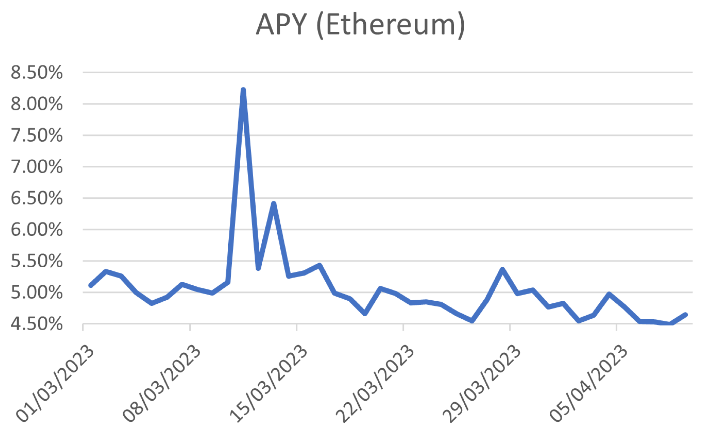
4.5.4. Implementation

We show the evolution of the APY with respect to time in Figure 2, from March 2023 to May 2023. The needed data (mainly g and $\chi$) are the one on-chain.

In Figure 2, the APY can vary abruptly based on the economic environment. Here, for instance, the spikes might relate to the US banking crisis—Silicon Valley Bank and Signature Bank—in March. This might be because the investors were looking to move their funds out of relatively higher-risk assets, especially since both these banks were heavy lenders to the technology sector, thus the spill-over effect. This assumption would need further testing to be properly validated and is out of the scope of this article. However, the main reason for such spikes observed in Figure 2 is likely due to the Shanghai release allowing withdrawals and increasing reward (g increased) [24,25].

4.6. Mining Rate Derivation

The cash-flow discount models in a PoW context seem to be more disputable. The underlying economic environment is quite different this time: staking is about depositing to receive an expected reward, while working consists in spending electricity to find a relevant nonce and connecting the latest block to the miner’s candidate block. A working probability space is defined the same way as in Section 4.1. In addition, if we still want to focus on an equation of the style of Equation (8):

$${\displaystyle P_i^{\prime }=\sum _{n=1}^{+\infty }\frac{G_{i,n}}{{(1+r)}^{t_n}},}$$

(20)

where $G_{i,n}$ represents the gain earned by miner i at time $t_n$, and $P_i$ is the present value of the total future gains, then the rate r is the return of gains obtained by spending money by a participant. To some extent, mining is like participating in a game by paying to earn reward and, contrary to staking, the payment of the game is continuously performed over time.

There are $\mathcal{N}\in {\mathbb{N}}^{*}$ miners in total. For all $i\in 〚1,\mathcal{N}〛$, we introduce the random variable $X_i$ to be the time for miner i to mine the coming block, i.e., be the first one to find a nonce among the pool of miners. The random variable $X_i$ can be assumed to have the memoryless property [18], and since it is a continuous and positive random variable, then $X_i\sim \mathrm{Exp}{\lambda }_i$, with ${\lambda }_i\in {\mathbb{R}}_{+}^{*}$ for all $i\in 〚1,\mathcal{N}〛$. Concretely, ${\lambda }_i$ represents the hash rate for miner i: the higher the rate, the less time miner i takes to mine its block. Henceforth, ${\displaystyle \Lambda =\sum _{i=1}^{\mathcal{N}}{\lambda }_i}$ is the total hash rate, and if $\Delta t>0$ is an arbitrary time period of mining, then $R=\Lambda \Delta t$ is the total hash computed by the set of miners during $\Delta t$. It is, therefore, the total cost for the whole mining activity.

Bearing this in mind, we have the main claim for this section.

Claim 4. 

If g is the average reward per block and R is the total hash to get this block constructed, then the $\mathrm{working}$ $\mathrm{rate}$ r is given by:

$$\begin{array}{|c|}\hline r=\frac{g}{R}\\ \hline\end{array}$$

(21)

Proof. 

First, we would like to prove that

$$\mathbb{P}\left(X_i<\underset{j\in 〚1,\mathcal{N}〛\setminus \left\{i\right\}}{\min }{X}_j\right)=\frac{{\lambda }_i}{\Lambda },\forall i\in 〚1,\mathcal{N}〛.$$

(22)

In fact, if $\mathcal{N}=2$, by using the Bayes formula, we have

$$\begin{array}{cc}\hfill \mathbb{P}\left(X_1<X_2\right)& ={\int }_0^{+\infty }\mathbb{P}\left(X_1<X_2|X_2=x_2\right)\mathbb{P}\left(X_2\in \mathrm{d}{x}_2\right)={\int }_0^{+\infty }\left(1-{\mathrm{e}}^{-{\lambda }_1{x}_2}\right)\times {\lambda }_2{\mathrm{e}}^{-{\lambda }_2{x}_2}\mathrm{d}{x}_2\hfill \\ \hfill & =1-\frac{{\lambda }_2}{{\lambda }_1+{\lambda }_2}=\frac{{\lambda }_1}{{\lambda }_1+{\lambda }_2}.\hfill \end{array}$$

Now, by mathematical induction, we can prove that ${\displaystyle \underset{j\in 〚1,k〛}{\min }{X}_j\sim \mathrm{Exp}\left(\sum _{j=1}^k{\lambda }_j\right)}$, for any $k\in 〚1,\mathcal{N}〛$. Bearing this in mind, replacing $X_1$ with $X_i$ and $X_2$ with $\underset{j\in 〚1,\mathcal{N}〛\setminus \left\{i\right\}}{\min }{X}_j$ gives Equation (22).

By going through the spirit of proof of Claim 1, for a fixed miner i and time $t_n$, we have

$$G_{i,n}=\mathbb{P}\left(\mathrm{miner}i\mathrm{finds}\mathrm{nonce}\mathrm{before}\mathrm{the}\mathrm{others}\right)\times g.$$

Here, we have

$$\mathbb{P}\left(\mathrm{miner}i\mathrm{finds}\mathrm{nonce}\mathrm{before}\mathrm{the}\mathrm{others}\right)=\mathbb{P}\left(X_i<\underset{j\in 〚1,\mathcal{N}〛\setminus \left\{i\right\}}{\min }{X}_j\right),$$

and g is the average reward, or

$$G_{i,n}=\frac{{\lambda }_i}{\Lambda }g.$$

From Equation (20), we have

$${\displaystyle P_i^{\prime }=\sum _{n=1}^{+\infty }\frac{1}{{(1+r)}^n}\frac{{\lambda }_i}{\Lambda }g=\frac{{\lambda }_i}{\Lambda }\frac{g}{r}.}$$

During $\Delta t$, the total investment is ${\lambda }_i\Delta t$, and thus ${\mathcal{P}}_i=P_i^{\prime }-{\lambda }_i\Delta t=0$ finally leads to

$$r=\frac{g}{\Lambda \Delta t}=\frac{g}{R}.$$

□

5. Discussion

5.1. Time-Dependency

It is worth pointing out that our approach is applied each time one needs to estimate the staking rate r. In practice, an update is performed each time a new block is added to the blockchain, giving a time series of the staking rate with respect to the block number. In particular, the number of total staked coins $\chi$, the award g, the slash rate s and the proportion q of burnt coins need to be updated systematically.

5.2. General Discussion on the Approach

We provide a rigorous mathematical foundation for modeling the staking rate, open to practitioner and academic scrutiny. More specifically, in order for the probability of an event and for the mathematical expectation to make sense, we pose the problem in the way of Section 4.1. Without a clear understanding of the underlying probability space, the model may produce misleading or inconsistent outcomes. From a business perspective, defining a probability space provides a common language for communication and collaboration among professionals. It ensures that the assumptions and interpretations of probabilities are clear and consistent across individuals or teams, fostering effective teamwork and minimizing misunderstandings. Last but not least, although this problem positioning may sound heavy, it appears necessary when considering the slash rate in the stake rate derivation: the definitions of ${\mathcal{W}}_{i,n}$, ${\mathbb{S}}_i$ and ${\mathbb{S}}_{i,n}$ do not appear ambiguous.

5.3. Adding Maturity

The rate will remain unchanged if one adds a maturity to our cash-flow discount model (here, a maturity represents the time when the staker retrieves their staked coins and thus stops being a staker). To see this, suppose $T_N$, for $N\in {\mathbb{N}}^{*}$, is the time at which the staker stops investing. Equation (8) becomes

$${\displaystyle P_i=\sum _{n=1}^N\frac{\mathbb{E}\left({\mathcal{G}}_{i,n}\right)}{{(1+r)}^{t_n}}+\frac{X_i}{{(1+r)}^{t_N}}.}$$

(23)

Then, the equation ${\mathcal{P}}_i=0$ leads to the same expression r for the rate as in Equation (7).

We have two remarks: (i) $X_i$ can be interpreted as the par of the investment, and (ii) regardless of whether the staker decides to stop their investment or not, the staking rate is the same. This is expected as long as we calculate a rate of return.

5.4. Assumptions and Healthy Blockchain

In the whole study, we assume that the blockchain is remaining sufficiently stable over time: it is not supposed to have substantial changes (e.g., no fork) or collapse. We are also not integrating attack events in our model, so we assume a blockchain which has a sufficiently long history with many honest agents acting on it. Such a healthy blockchain is likely to survive for a sufficiently long time so that staking perpetually remains a relevant approximation. It is worth pointing out that a healthy blockchain and the memoryless property of intrinsic features (e.g., transaction fees) are two faces of the same coin. Intrinsically related to this main assumption, the reward dates are supposed to be known in advance (as suggested by the equation $t_n=n$ for all $n\in \mathbb{N}$) and the blockchain is supposed to continue to pay the rewards indefinitely (see, for example, Equation (8)). In addition, Equation (8) also suggests that a constant actualization rate is applied to value the infinite stream of rewards, i.e., the staking rate r is constant in the actualization of the rewards, which are thus supposed to be reinvested systematically each time they are earned.

5.5. Model Limitations

The main assumption of this model, as discussed above, is that it operates only on healthy blockchains. The perpetual characteristic of the bond approach uses the assumption of a sufficiently stable blockchain in time. This cannot happen if the blockchain is either forked or attacked, that is, if there is any specific change—i.e., rule breaking—which makes the blockchain have a different behavior from the one expected when calculating the rate. Thus, the model cannot apply if the blockchain will not continue to pay the rewards indefinitely (however, this aspect of the model is flexible by implementing some maturity; see above). From a perfectly healthy blockchain, which implies the stability of the whole system over time, the idea is to add more and more of what is making the blockchain less healthy, among which include a lack of hardware, or attacks. However, the first needed feature to consider—as it is inherent to staking—is slashing.

5.6. Slashing

Although the formula $r=g/\chi$ might appear intuitive and trivial, the implementation of the slash rate into the process reveals an equation which was not easily expected (see Equation (15)): the first term is a quadratic decrease in the gain, while the second one is a linear decrease, with the slope being the proportion of burnt stake coins. Overall, the staking rate is a decreasing quadratic function of the slash rate. One might think that the staker is taking more risks by staking since they can lose the initial investment, and thus, the reward should increase. However, the context is quite different from standard cash-flow discount models: the investor themselves can enhance a false or wrong validation process. Thus, the decrease in the staking rate can be seen as an average penalty included in the rate.

In addition, we have assumed that the staker is banned from the blockchain, which is not necessarily true: the staker can only have a proportion of burnt coins, remaining a staker as long as they still have staked coins remained in the staking pool. It would be interesting to see what Equation (16) would become then. We would need to introduce the cumulative slashing time ${\mathcal{N}}_{i,p}$, which is the time staker i has been slashed for the $p^{\mathrm{th}}$ time, $p\in {\mathbb{N}}^{*}$, i.e., to simplify:

$${\mathcal{N}}_{i,p}=\sum _{m=1}^p{N}_i=p{N}_i,$$

where we assumed time independence between two consecutive slashes. Since $N_i$ is the time of slashing for staker i, then $p{N}_i$ is the time for being slashed p times. Thus, Equation (16) becomes:

$$P_i=\mathbb{E}\left(\sum _{n=1}^{+\infty }\frac{{\mathcal{G}}_{i,n}}{{(1+r)}^n}+\sum _{p=1}^{+\infty }\frac{X_i{(1-q)}^p}{{(1+r)}^{{\mathcal{N}}_{i,p}}}{\mathbb{S}}_{i,{\mathcal{N}}_{i,p}}\right).$$

(24)

The first term leads to $X_{i}g/\chi r$ (see Equation (10)), while the second term would write as (inverting sum and expectation and setting ${\mathbb{S}}_{i,{\mathcal{N}}_{i,p}}=1$):

$$\mathbb{E}\left(\sum _{p=1}^{+\infty }\frac{X_i{(1-q)}^p}{{(1+r)}^{{\mathcal{N}}_{i,p}}}{\mathbb{S}}_{i,{\mathcal{N}}_{i,p}}\right)=\sum _{p=1}^{+\infty }{X}_i{(1-q)}^p\mathbb{E}\left(\frac{1}{{(1+r)}^{p{N}_i}}\right)=X_{i}s\sum _{p=1}^{+\infty }\frac{{(1-q)}^p}{{(1+r)}^p-(1-s)}.$$

Unfortunately, there is no close formula for the sum above, to the best of our knowledge. In fact, in our model, we do not pretend that a slashed staker will never be able to come back through another round, perhaps after some time. The above calculation could be more complicated, but we do not believe it is necessary for what we want to achieve in this study.

5.7. Memoryless Property for Slashing Events

In Section 4.3, we assumed that stakers can be slashed in a time-independent way. Stakers can be slashed for various reasons, e.g., double signing (validation of conflicting transactions), downtime (offline staker, not able to validate while selected), or non-compliance (failure to follow the protocol rules). Despite the fact that the exact slashing conditions depend on the specific rules of each blockchain protocol, there is no evidence, to the best of our knowledge, that there is a spontaneous time dependency in the slashing process for individual stakers. Time dependency appears due to a common decision for forking, or due to an attack provoking radical protocol changes. We are assuming a healthy blockchain, though we do not consider these events to occur.

5.8. Slashing Event Independent of Staker

In Section 4.3, we assumed that the slash rate was independent of i. This can be seen as an approximation, as this supposes that stakers all have the same resource and implementation of the verification and validation processes. However, it remains difficult to evaluate individual abilities to correctly validate blocks. In addition, for Ethereum, the staking amount is the same for all stakers, that is, ETH 32, which means (i) the process tends to provide equality of chance of selection, and (ii) resources may be comparable.

5.9. MEV and Total Income

MEV represents a significant portion of the stakers’ income in a high-traffic network like Ethereum 2.0. We have provided an estimation of the income g only from MEV, in Section 4.5. However, the specific income can vary widely. Some cryptocurrencies offer a fixed percentage of returns for staking their coins, whilst others fluctuate based on network usage and transaction volumes. To obtain more specific numbers, one would need to look into individual coins’ staking models and rewards. Thus, it seems difficult to provide a general income model, as one can find strong variability within PoS blockchains. However, we think our approach generally captures the idea of MEV as a classification of transactions with respect to their transaction fee amount, allowing increasing reward gains.

5.10. Transaction Fee—Exponential Assumption

In Section 4.4, we assumed that the transaction fee was represented by a random variable whose law is an exponential one. This is a consequence of the discussion depicted therein about the memoryless process. Having an estimation of F would require to have access to a sufficiently large number of transaction fees at a given time. If the collected sample is a sufficiently good representation of the whole population, the average transaction fee $\theta$ would be close to its true value, and, more generally, we would have access to a broader distribution of transaction fees. Only then would we be able to have an idea of the distribution of the transaction fees, i.e., if they follow an exponential law rather than a log-normal one. Below, we have, however, performed a fit to the distribution of daily average transaction fees (in ETH) for the Ethereum blockchain (see Figure 3). The data were selected from 7 November 2022 to 7 November 2023 on Blockchair (https://blockchair.com). The time period corresponds to Ethereum 2.0 and is a relatively long time after the fork, allowing more stability in the chain data. We fit the exponential and lognormal distributions to the data histogram; the other distributions (e.g., normal) do not have enough significance to be shown here. In Figure 3, we rescale the distributions to the empirical histogram so that both fits can be shown in the same figure.

The fits are using the fitdistr function in R (optimization based on Nelder–Mead, quasi-Newton and conjugate gradient algorithms). We show three fits: (i) fitting the exponential law with the tail (from the median of the distribution), (ii) fitting the log-normal law with the whole distribution, and (iii) fitting the log-normal law with the tail. The Kolmogorov–Smirnov test (null hypothesis: data can be fitted) reveals a p-value below 0.05 for the second case, and p-values largely above 0.05 for the other cases (see caption in Figure 3). Thus, within the 95% level confidence, we can reject the null that the whole data are fitted with a log-normal distribution, while we can reject the alternative that the tail is not fitted with exponential and log-normal distributions. Given the model depicted in Section 4.4, we consider large values for transaction fees (m can be chosen in a way to focus on values which are fitted with exponential laws). Thus, we cannot reject the exponential assumption for the tail of this data set. It is worth stressing that this above fit is already assuming the memoryless property: the distribution is taken over time, rather than at a given time.

5.11. Mining Rate

Conceptually, it is interesting to have a mining equivalence of the cash-flow discount approach. We still can derive a rate, not in a sense of investment, but rather as a ratio of ‘gain for mining a block/expense to mine’. However, contrary to the staking rate, where alliances between pool operators and depositors usually occur, it does not look straight to emphasize some business utility from the mining rate.

6. Conclusions

As investor interest has increased over time, the formalism of a standard crypto yield model for staking return has become an industrial need. In this paper, we proposed an approach for a PoS consensus blockchain to model the staking reward. We have used the cash-flow discount model for the calculation of the staking rate, given by the ratio of the average reward out of the total staked coins. Essential addons, the likes of which include slash events and MEV, complemented the model, and an illustration for the Ethereum blockchain was proposed. The same approach was applied to a PoW consensus blockchain, and the resulting working rate is the ratio of average reward out of total hash, which resembles the PoS ratio. We discussed the assumptions made in our model and further illustrated with an empirical study. The main assumption is a healthy blockchain, sufficiently stable over time and robust against attacks and decisions of rule changes.

We believe that this rate methodology should become an industrial standard, as it will allow the derivation of futures prices and the construction of yield curves in a consistent way. In the middle term, this approach should enhance the implementation of swaps for the obtention of more accurate and stable term structures. The resulting infrastructure could improve the tradability of crypto derivatives and further stabilize the market.