Abstract
Anthrax is a highly fatal zoonotic disease that affects all species of livestock. The study aims to develop an early warning of epidemiological anthrax using machine learning (ML) models and to study the effect of El Niño and La Niña oscillation, as well as the climate–disease relationship concerning the spatial occurrence and outbreaks in Karnataka. The disease incidence data are divided based on El Niño and La Niña events from 2004–2019 and subjected to climate-disease modeling to understand the disease pattern over the years. Machine learning models were implemented using R statistical software version 3.1.3 with Livestock density, soil profile, and meteorological and remote sensing variables as risk factors associated with anthrax incidence. Model evaluation is performed using statistical indices, viz., Cohen’s kappa, receiver operating characteristic (ROC) curve, true skill statistics (TSS), etc. Models with good predictive power were combined to develop an average prediction model. The predicted results were mapped onto the Risk maps, and the Basic reproduction numbers (R0) for the districts that are significantly clustered were calculated. Early warning or risk prediction developed with a layer of R0 superimposed on a risk map helps in the preparedness for the disease occurrence, and precautionary measures before the spread of the disease.
1. Introduction
Anthrax is an acute, infectious, non-contagious, zoonotic disease that remains a threat to public health throughout the world. The causative agent of anthrax is Bacillus anthracis, which is a rod-shaped, spore-forming, soil-borne bacterium that survives in the soil under suitable conditions for long periods of time [1]. B. anthracis is an extracellular pathogen that replicates rapidly in the blood, conquering high density to make the host diseased [2]. The soil pH, organic calcium, potassium, and zinc concentrations of soil are believed to be correlated with the survival of spores [3]. Animals come into contact with the spores by grazing grass closer to the surface when the grass is low or scarce, or by moving herds to restricted areas when water is scarce [4]. The disease has not been eradicated in humans and livestock in most African and Asian nations, in several southern European countries, the Americas, and some Australian regions [5]. There is a slight dispute that anthrax is a disease that occurs only at certain times of the year, and its occurrence in any particular location is associated with temperature, rainfall or drought, soil, and vegetation. Nevertheless, the literature documents that the conditions which influence outbreaks vary broadly from location to location [4]. Many diseases that are viral, parasitic, and bacterial respond to climate patterns, distribution of geography, inter-annual fluctuations, seasonality, or spatial and temporal patterns [6]. Many of the world’s endemic diseases like anthrax are known to be very subtle to long-term variations in climate. The application of ecological data to the study of disease exhibits the relationship between disease and the environment, and also helps to potentially predict the risk of disease outbreaks [7,8]. Variations in the climate of a geographical region can be the consequence of several different environmental incidences, comprising teleconnections [9]. Teleconnections are the concurrent variations in climate patterns around the various regions of the globe. One example is the El Niño-Southern Oscillation (ENSO), and it is considered one of the most vital factors that drive inter-annual global climate variability [10]. Sea surface temperatures (SSTs) in the tropical Pacific Ocean can change significantly from extraordinarily warm (El Niño) to cold (La Niña). El Niño and La Niña periods typically last between two and seven years and are caused by significant fluctuations in the Southern Oscillation, a pattern of air pressure that covers the tropical Indian and Pacific Oceans [11]. The Indochina region is severely impacted by both El Niño and La Niña seasons, which alter temperature, rainfall, and other weather-related factors such as the occurrence of tropical cyclones. The influence of El Niño and La Niña on Southeast Asia, 2000: Despite the possibility of some positive impacts, harmful effects on crop yields, water supply, the possibility of floods and storms, and other factors that affect human well-being and economic strength occur frequently. Indisputable ENSOW (El Niño years, where the Pacific Sea’s temperature reached its highest point and the Southern Oscillation Index reached its lowest point) were more strongly linked to droughts [12].
Since 1950, a total of 23 El Niño and 13 drought years were recorded, among the 13 drought years, only 3 were in non-El Niño years. Since 1980, most Indian droughts have occurred during El Niño years, while not all El Niño years have seen droughts [13]. A prime illustration of this was the drought in 2002, which had been accompanied by such a strong El Niño and resulted in a more than 19% decrease in Indian monsoon rains from its long-period average (LPA). Food grain output declined by 18% (38 million tonnes), while agriculture’s contribution to GDP fell by 7% (a loss of almost USD 8 billion) [13]. ENSO had a variety of effects on rainfall and rice productivity in different districts of Karnataka state. Southwest (S-W) monsoon rains have been below average in all of Karnataka’s districts throughout El Niño (strong, moderate, and mild) years, with the Mysore district showing the biggest negative divergence from average (21.43%). In contrast, out of 25 districts, 15 had higher rice output than the national average, with the Gulbarga district having the highest divergence from normal at 42.11%. The S-W monsoon rains have been above average during the La Niña (strong, moderate, and weak) years in 12 districts, with Bengaluru urban and Bidar districts recording the highest positive deviations (19.82% and 19.93, respectively) [14].
Globally, ENSO has an impact on inter-annual variation in weather patterns and the possibility of regional extreme weather events such as droughts and floods [15]. The incidence of multiple infectious diseases in endemic areas may be impacted by global changes in temperature and precipitation trends in various locations, according to forecasts from the Intergovernmental Panel on Climate Change (IPCC). Nonetheless, various factors, such as a rise in the migration of animals between regions and countries, animal trades and animal products, etc., may also have an impact on these alterations [16].
Early alert for epidemics refers to the formulation of risk or modeled forecasts of possible outbreaks based on systematically collected data from the monitored sites to allow for effective and timely prevention and response actions. Climate-based early warning of the disease has been anticipated as a potential tool in climate change adaptation for the health sector [6]. Accurate disease prediction models would markedly improve epidemic prevention and control capabilities [7]. Early warning or risk prediction in the medical and livestock sector is not only a feasible but necessary tool to battle the re-emergence and spread of infectious diseases. Consequently, machine learning is one of the most promising technologies of artificial intelligence (AI) applications that played a key role in biomedical, especially in the area of disease prediction to deal with big data, due to the availability of numerous algorithms to solve complex problems [17]. The ability to predict epidemics would provide a methodology for governments and healthcare providers to react to outbreaks quickly, minimizing the effects and conserving scarce resources.
The variations of different land use in a landscape reveal current and historical processes that shape the landscape’s dynamics and organisation, and also spread the disease ability. Recognizing this dynamic behavior is also important in light of the impacts of climate change. These days, remotely sensed data quests carried out by various private and public organizations allow for the monitoring and quantification of environmental changes at various space-temporal resolutions. Precise information about the origin and destination of both the growing season of vegetation would be extremely crucial for monitoring and modeling the consequences of climate change on ecosystem functioning [18,19].
Descriptive observations and satellite measurements could be used to support study results on growing period variability. Many such public health study results in Africa and Asia used GIS to identify environmental factors, particularly vector-borne diseases. Worldwide satellite-based surveillance of appropriate climatic parameters could aid in mapping occurring anomalies with the goal of forecasting the spatial distribution of risk associated with disease occurrence and spreading. Such data can provide enough time to prevent outbreaks and conceivably reduce the impact and spread of environmentally associated diseases [18].
Remote sensed data are currently being used by epidemiologists to conduct an investigation of a wide range of vector-borne diseases. To map and characterize vector habitats, correlations among specific node meteorological factors (e.g., temperature, humidity, land cover, etc.) as well as vector density are used. The fundamental concept would be that data collected remotely could contain dynamic predictor variables of Earth’s processes that can be utilized to describe niche priorities of certain medically significant factors affecting disease processes. Furthermore, due to the consistency with which they are acquired, remotely sensed information includes a synoptic depiction of the environment at appropriate temporal and spatial scales [18,19,20].
The current study aims to analyze anthrax cases in livestock animals between 2004 and 2019 to understand spatio-temporal persistence and disease burden over the past decades, directional trend, identify the significant presence of disease clusters and find the effect of El Niño and La Niña oscillation in early warning of an anthrax outbreak among livestock in the state of Karnataka, India, using machine learning models.
2. Materials and Methods
2.1. Data Collection
2.1.1. Disease Incidence and ENSO Events Classification
The Incidence is usually expressed as a rate and is a measure of the frequency in which a disease or event occurs in a given population over a given period [21]. The current study includes the incidence data of anthrax among livestock throughout Karnataka. Incidence data is divided into two sets based on ENSO events. National weather service climate prediction center, the website https://ggweather.com/enso/oni.htm (accessed on 8 February 2021) was used to obtain information on ENSO events. The Oceanic Niño Index (ONI) has become a widely acknowledged criterion for distinguishing El Niño (warm) and La Niña (cool) episodes in the tropical Pacific by the National Oceanic and Atmospheric Administration (NOAA). The Niño 3.4 region (i.e., 5° N–5° S, 120–170° W) has an ongoing 3-month mean SST anomaly. Events are classified as 5 sequential overlapping, 3-month periods that are either at or below the −0.5° anomaly for cold events (La Niña) are either at or above the +0.5° anomalies for warm events (El Niño).
As a result, the study periods were categorized as El Niño and La Niña years based on the occurrence of ENSO events. There were six El Niño events (2004, 2006, 2009, 2014, 2015, and 2018) and seven La Niña events (2005, 2007, 2008, 2010, 2011, 2016, and 2017) that occurred between 2004 and 2020 (Figure 1).
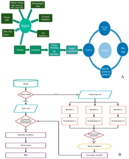
Figure 1.
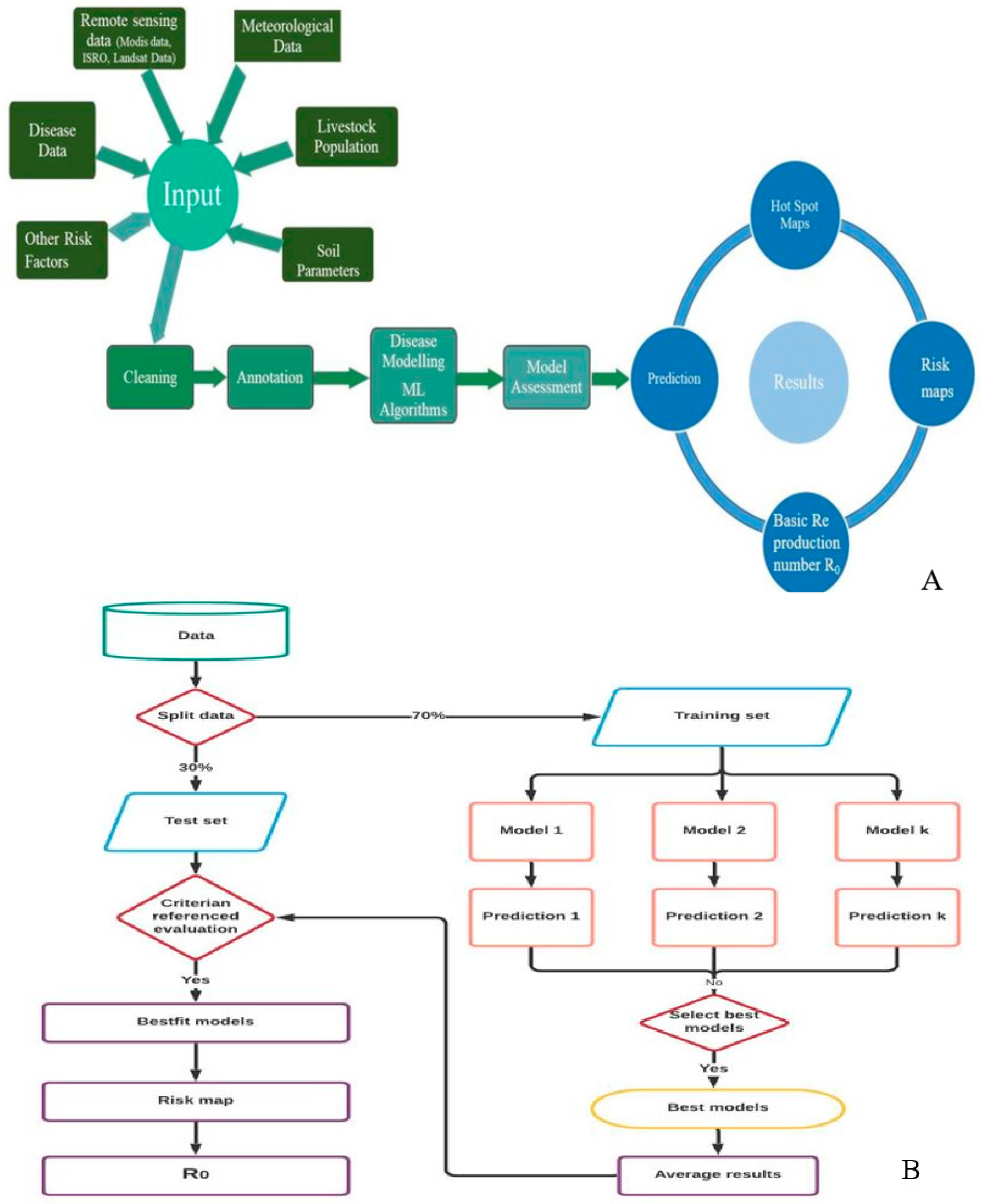
(A) Diagrammatic representation of machine-learning powered early warning. (B) Flowchart depicting the risk modeling and risk mapping.
Karnataka is a state in India with 191,791 km2 area, 181 blocks spread across 30 districts, and 29,340 villages holding 27.7 million livestock animals. The current study included all 30 districts of the state over the period of 2004–2019. The village-level livestock anthrax outbreak data were retrieved from the Dept. of Animal husbandry, Bengaluru, Karnataka, India. The outbreak data were spatial and temporal referenced and cross-checked for coordinate data (X, Y), species, district codes, and month of occurrence and cleaned for all types of errors before storing the data in a database.
2.1.2. Livestock Data
India has an abundance of livestock, with around 535.78 million animals overall, of that which 192.49 million comprise cattle and 50.42 million are exotic/crossbred. In fact, there are 109.85 million buffaloes, 9.06 million pigs, 148.88 million goats, 74.26 million sheep, and 0.44 million Mithun and yaks. (Department of Animal Husbandry & Dairying (DAHD)- 20th Livestock Census of India). The livestock population data throughout Karnataka in five major animal species, i.e., cattle, buffalo, sheep, and goats, were collected from the 20th livestock census of India at the village level.
2.1.3. Meteorological Data
The Meteorological/remote sensing parameters include soil moisture (kg/m2), potential evaporation rate (w/m2), specific humidity (kg/kg), rainfall (kg/m2/s), air temperature (k), wind speed (m/s), and surface pressure (pa). These parameters were obtained from the Global Land Data Assimilation System https://ldas.gsfc.nasa.gov/gldas (new and reprocessed GLDAS version 2) (accessed on 10 February 2021), which uses advanced land surface modeling and data integration methods to capture satellite and ground-based observed data with a spatial resolution of 0.25° × 0.25° and a temporal resolution retrieved in network common data format (netCDF). This includes metadata as well as data that have a multidimensional array and data dimensions. The data were extracted using the ‘ncdf4’ package in the R tool.
2.1.4. Remote Sensing Data
The method of detecting and tracking the physical characteristics of an environment by measuring its emitted and reflected radiation from a distance is known as remote sensing [22]. Remote sensing data from the Moderate Resolution Imaging Spectroradiometer (MODIS) satellite include the enhanced vegetation index (EVI, 16-day interval), potential evapotranspiration (PET, 16-day interval, 500 m), land surface temperature (LST, 8-day interval, 1 km), normalized difference vegetation index (NDVI, 16-day interval, 500 m), potential leaf area index (LAI, 16-day interval, 500 m), and were extracted with image products such as MOD16A2, MOD11A2, MOD13A1, and MOD15A2H [23,24]. These parameters are downloaded in HDF format with different spatial and temporal resolutions. The data were extracted as HDF files and converting them to GeoTIFF files using the R packages “gdalutils” and “modis”. Each prediction must be a raster layer reflecting the variable of interest. All the variables are arranged as raster (grid) style files by using the R package “raster” [25]. Remote sensing data is collected and divided into two different data sets based on El Niño and La Niña years between 2000 and 2019.
2.1.5. Soil Profile
The soil profile is a vertical section of the soil that depicts all of its horizons. From the soil surface to the parent rock material, the soil profile is measured. Some variations in animal health among geographic areas are associated with variations in soils and their properties [26]. Some animal infectious diseases’ origin may be from particular soils, and more direct effects may be expected if the pathogen can survive, grow, and reproduce in the soil [27]. The database of Karnataka soil health data (ICRISAT Development Centre, Government of Karnataka, 2016) was used to obtain the soil parameters used in the current study, which include potassium, phosphorus, boron, zinc, sulphur carbon, and pH.
2.2. Spatial Endemicity
The year-wise outbreak of anthrax was analyzed to understand the disease occurrence pattern related to spatial and temporal endemicity [28]. The study period was grouped into two groups based on El Niño and La Niña years to identify potential changes in the reporting of the disease over time and space. The cumulative outbreak of cases was represented at the village level using R software for each El Niño and La Niña year from 2004 to 2019.
2.3. Getis-Ord Gi* Spatial Statistics to Identify Hotspots (Spatial Autocorrelation)
The use of Getis–Ord (Gi*) spatial statistics classified hotspots on freeways from an IM database when considering selected impact attributes. Within the context of the conceptualized spatial relationship, the Gi* spatial statistics jointly measure the spatial dependence effect of the frequency and attribute values [29]. Getis Ord’s Gi* statistics were used to detect the evidence of any spatial clusters. Getis Ord’s Gi* statistics can accurately discriminate between hot spots and cold spots. In spatial autocorrelation, spatial units that are close together have more in common than units that are far apart [30], and it investigates the covariations for the properties of observations within a two-dimensional geo-surface in the study area. Spatial autocorrelation was performed in the present study to address the problems associated with spatial units that bear some measurable attributes [31]. The Getis Ord’s index was calculated using the statistical program R. When the GI value is more than 0, a clustered pattern is observed, and when it is less than 0, a dispersed pattern is observed.
2.4. Space-Time Cluster Analysis
To detect the temporal, spatial, and space-time clusters of anthrax in Karnataka for 16 years, the Poisson-based clustering models based on space-time scan statistics were implemented in SaTScan software v9.6. In the case of SaTScan, to detect spatial clusters across a study area, a series of moving windows with varying diameters are used, likewise, temporal clusters are detected and it places ellipses or circles of constantly varying sizes over a three-dimensional study area [32,33]. The circles with observed values that are higher than expected values are reported as clusters. They can be used in a variety of settings and come in a variety of sizes. In order to conduct cluster analysis on a dataset with each parameter having a disease status (case vs. control), along with spatial and temporal properties, for the SaTScan studies, village-wise latitude and longitude coordinates were taken into consideration [34]. The model had been applied to the case dataset for each year, using the total number of cases for each epi unit (village) in a specific year while accounting for the actual population of each epi unit with a significance value of (p ≤ 0.05) in SaTScan.
2.5. Identifying Risk Factors by Linear Discriminant Analysis
Linear discriminant analysis (LDA), a modified algorithm based on Fisher’s linear discriminant, is a technique used in statistics and machine learning to distinguish between two or more classes. The risk parameters were thoroughly analyzed using discriminant analysis, and the mathematical relationship among them was developed to provide a solid base for precisely understanding the influence of the parameter on its calculation and prediction [35]. LDA was used to determine whether there were any differences in risk factors between regions where a persistent and non-persistent space-time cluster was found to exist using SaTScan. LDA was used to assess a maximum of 12 environmental/remotely detected factors using a binary response (0/1) with clustered regions equal to 1 and non-clustered regions equal to 0, respectively. In this study, the LDA was performed with R programming language, with a statistical significance of (p ≤ 0.05) for all the parameters.
Linear discriminate analysis for multiple classes:
where: Sk = scatter matrix
X = number of samples
Sw = within class scatter
C = number of distinct classes
where: Sb = between class scatter
m = mean of all the data points
2.6. Risk Modelling and Mapping
Data on risk factors generated over 16 years (2004–2019) were pooled at the grid level. Climate–disease correlation modeling was used to generate the risk map (2004–2019) for the Karnataka state, which estimates the disease’s spatial incidence. The information on risk factors was acquired, subjected to pre-processing, and annotated with disease conditions and thus the corresponding latitude and longitude.
To generate the most accurate prediction with enhanced performance, risk estimation is performed employing machine learning models. Due to overfitting or underfitting, ML models frequently may not operate effectively. The overfitting or underfitting of a model is decided by a bias-variance trade-off. The overall error of a model is dependent on the bias and variance of the model. Bias is an error from erroneous assumptions in the learning algorithm. Due to high bias, an algorithm can ignore important relationships between features and target outputs. Variance is an error caused by the training set’s vulnerability to minor variations. Because of the high variance, an algorithm will model the random noise in the training data instead of the expected outputs [36]. Random forest (RF), gradient boosting machine (GBM), artificial neural network (ANN), generalized linear models (GLM), generalized additive models (GAM), flexible discriminant analysis (FDA), support vector machine (SVM), multiple adaptive regression splines (MARS), naive Bayes (NB), classification tree analysis (CT), and adaptive boosting (ADA) are the eleven machine learning models employed in the current study for disease modeling. Predictions for combinations of predictor factors were generated using a range of model artifacts that were produced by different modeling techniques. Response graphs have been created in order to better interpret and evaluate model predictions. The discriminating capacity of the fitted models was evaluated using receiving operating characteristic (ROC) curve, Cohen’s kappa (Heidke skill score), true skill statistics (TSS), area under ROC curve (AUC), ACCURACY, ERROR RATE, F1 SCORE, and logistic loss (LOGLOSS). The accuracy of predictions based on the presence (1) or absence (0) of data was assessed using these metrics. The results of individual predictions by different model methods were combined using Raster Stack. All of the models’ overfitting was assessed as it may result in incorrect estimates of the coefficients, p-values, and R-squared values (<0.01 significant) [37]. Over-fitting is presumed to have occurred when the model accuracy is high for the training data but subsequently drastically decreases with new data [38,39]. In the current study, the cross-validation approach was employed to evaluate the over-fitting of models by keeping 70% of the data on the training set and 30% of the data on the testing set. It is suggested to use the combined prediction outcomes of several models, that are evaluated on a scale of 0 to 1, and average the score given the best prediction instead of focusing on a single prediction model. The overall average was determined by taking into consideration if the model satisfies the following criteria: kappa > 0.60, TSS > 0.80, ROC > 0.90, ACCURACY > 0.90, AUC > 0.90, ERROR RATE < 0.10, LOGLOSS < 0.30, and F1SCORE > 0.90 [40,41,42]. Different risks are connected with deviations from the normal pattern of meteorological and remote sensing factors, as well as soil parameters and densities of livestock in both space and time, which is depicted as a schematic framework for generating the risk map (Figure 1A,B).
2.7. Basic Reproduction Number (R0)
The estimated number of additional infectious disease cases that result from the initial incident in a community that is susceptible is known as the basic reproductive number (R0). The threshold of R0 is where its significance lies. The number of affected people will increase if R0 > 1. Additionally, the number will drop if R0 < 1. The transmission rate of a disease is expressed by R0. The basic reproduction rate is a pandemic’s common phrase since it explicitly reflects the virus’s nature. There are numerous methods available for the estimation of the R0 [43]. Maximum likelihood estimation (ML), exponential growth rate (EG), attack rate (AR), time-dependent method (TD), sequential Bayesian approach (SB), and various other methods can be implemented to calculate R0 [44]. In the present work, R0 was estimated using EG, ML, and AR approaches.
2.7.1. Exponential Growth Rate (EG)
The number of cases increases rapidly during the initial stages of an epidemic. The paradigm for exponential growth (EG) would be a condensed form. A rate of growth that continues constantly throughout time is referred to as exponential growth [45]. The basic reproduction number R0 could be deduced from the exponential epidemic growth curve. In the initial stages of an epidemic, R0 is associated with exponential growth as follows:
Here, r is the exponential growth rate and M is the moment-generating function of the GT distribution. Integers constitute the daily confirmed cases data. In order to obtain the value of the growth rate, r, Poisson regression is used [44].
2.7.2. Maximum Likelihood Estimate (ML)
White and Pagano’s maximum likelihood (ML) is predicated on the idea that the quantity of secondary cases caused by an affected individual is Poisson distributed, with R representing the expected value. Optimizing log-likelihood over an exponential growth phase yields R. The optimal period can be determined using the deviation R-squared metric. No assumption has been made about population mixing [46].
2.7.3. Attack Rate Estimate (AR)
The percentage of the population that gets an infection over time is referred to as the attack rate (AR) [46]. The basic reproduction number is related to AR by:
where s is the basic vulnerability rate of the population.
All of the methods are aimed to calculate the initial exponential growth from occurrence counts. Besides plotting the R0 on the anticipated risk maps, we gave a clear and in-depth insight into how a disease affects a specific area. Basic reproduction rate (R0) calculations were made using R statistical software (version 3.6.3). It is essential to evaluate a disease’s potential for transmission, predict the scale of epidemics, and spread awareness of preventative actions. Superimposing the R0 on the risk map predicted using the density of livestock, soil parameters, meteorological, and remote sensing parameters provides a visualized and comprehensive view of the likelihood and impact of a disease in a given region.
2.8. Statistical Software
R statistical software version 3.1.3 (version 3.4.3, Vienna, Austria: R Foundation for Statistical Computing) was used to perform statistical analyses, risk maps, and disease predictions. Data mining, computation, and graphical display were all done using R as an integrated suite. When data processing, integrating, annotating model fitting, and computing R0, the R packages plyr, dplyr, rgdal, raster, data.table, openxlsx, tmap, sp, spdep, sf, BAMM tools, foreign, geosphere, MASS, biomod2, dismo, mgcv, randomforest, mda, gbm, earth data extraction, data alignment, annotation, analysis, modeling, and risk mapping were all performed using Getis ord’s Index. SaTScan v9.6 was implemented to obtain the spatial and temporal clusters in the respective study area.
3. Results
3.1. Temporal Distribution of Weather Parameters
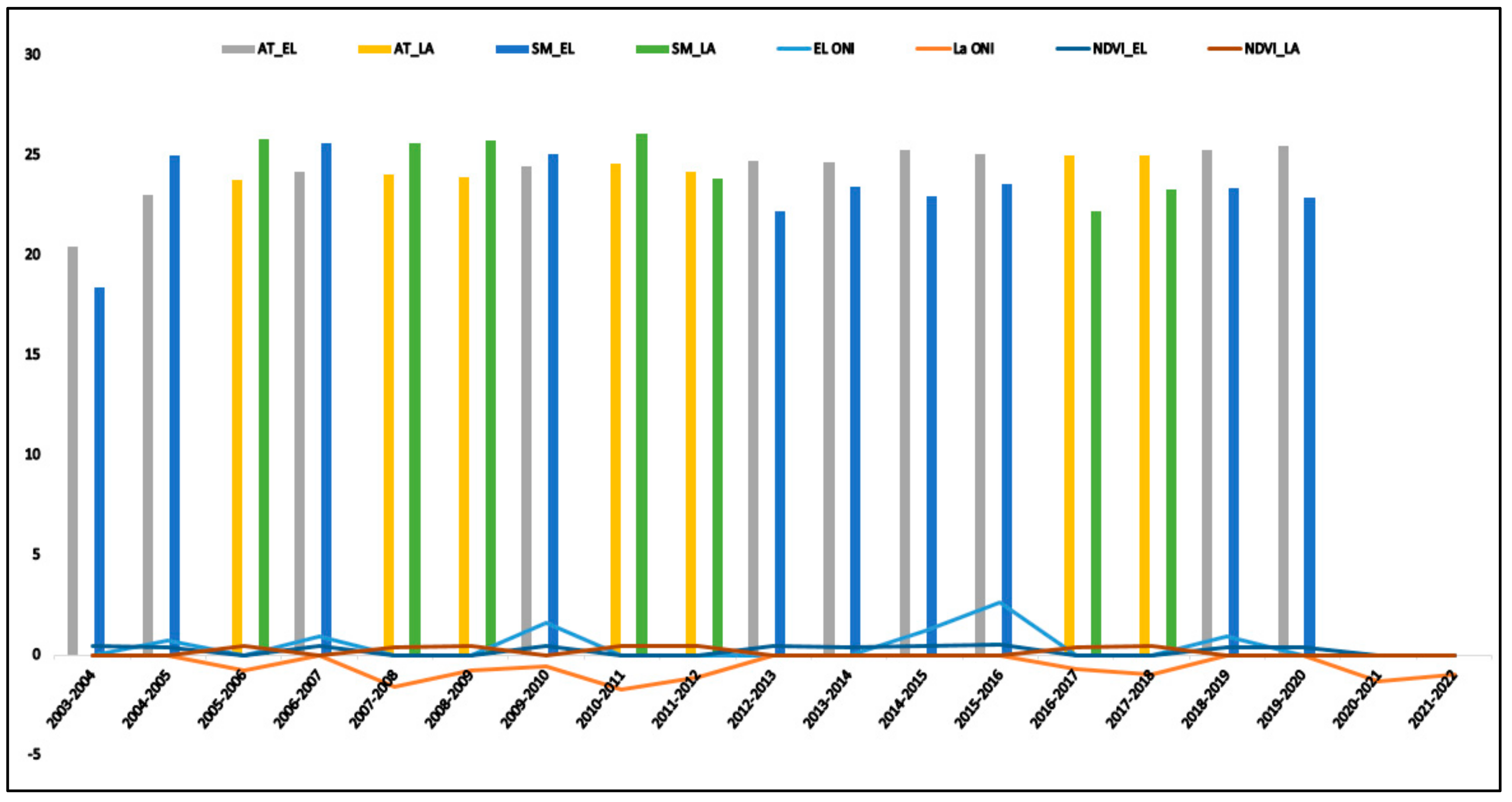
The temporal distribution of weather parameters viz., Air temperature, soil moisture, vegetative Index, El Niño, and La Niña oceanic index were plotted (Figure 2). The average sea temperature anomaly as captured under the ONIA for the 6 El Niño years was 0.41 °C, while that for the 7 La Niña years was −0.55°. The average air temperature for El Niño and La Nino years in the study year was 23.91 k and 23.16 k, respectively. The average vegetative index was 0.41 and 1.45 in El Niño and La Niña years, respectively (Table 1).

Figure 2.
Pattern of behavior of weather parameters in El Niño and La Niña.

Table 1.
Descriptive statistics of parameters included in the study from 2003 to 2020.
3.2. Spatial Endemicity of Anthrax
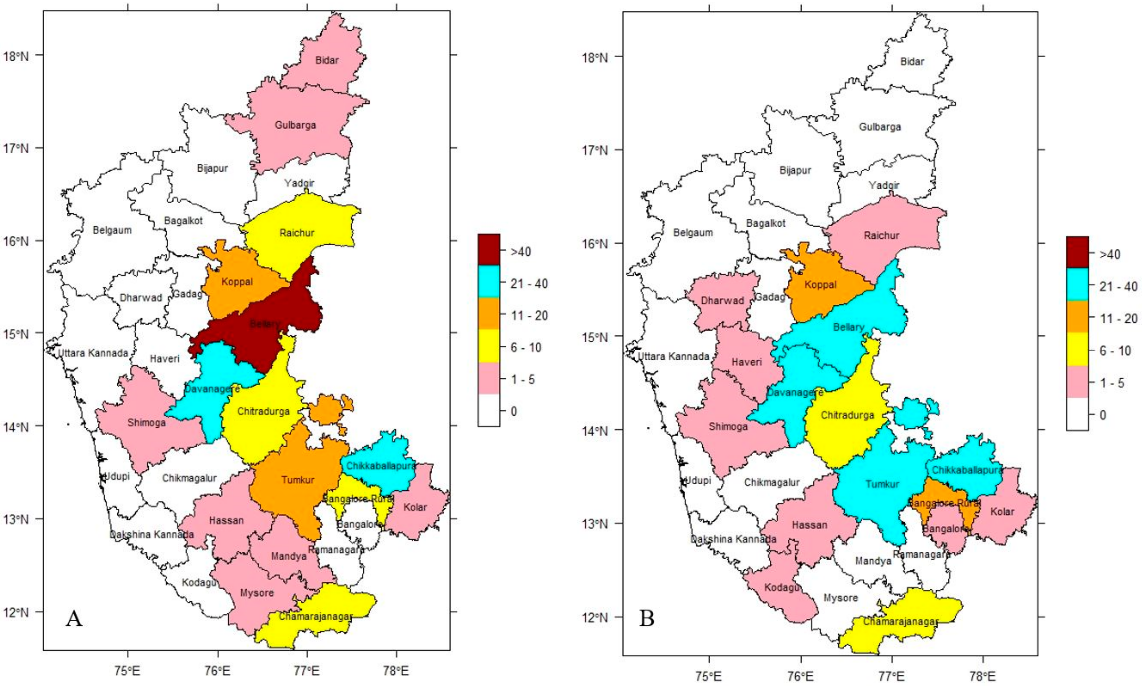
The dataset on the incidence of anthrax in Karnataka, India, throughout the 16-year study period ranging between 2004 and 2019 is split into two distinct sets based on ENSO events. Figure 3A,B illustrate the distribution of disease based on analysis of incidence data from El Niño and La Niña years, indicating the endemic nature of the disease in the study region. During the El Niño years, the highest incidence was observed in the Bellary district (range > 40) and moderately high incidence in Chikkaballapura and Davanagere districts (range 21–40). During the La Niña years, the highest incidence was not observed in any district (range > 40) and moderately high incidence was observed in Bellary, Chikkaballapura, Davanagere, and Tumkur districts (range 21–40). Despite the fact that anthrax in livestock continued to be a widespread disease throughout all of the years under study, the seasonal climatic pattern could be seen each year. The infection pressure was high during September and October in El Niño years and during August and September in La Niña years with September being the month where it peaks every year. During the winter, there was the lowest incidence of disease.
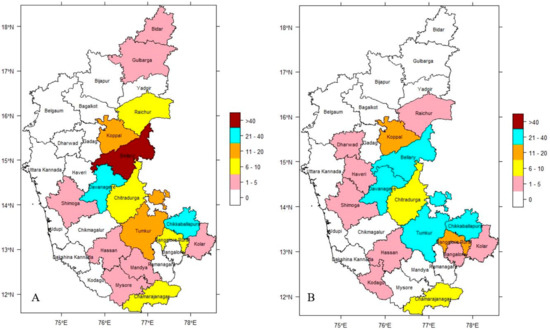
Figure 3.
District-wise cumulative incidence of anthrax in Karnataka (2004–2019), (A) El Niño years & (B) La Niña years, respectively.
3.3. Spatial Autocorrelation of Anthrax
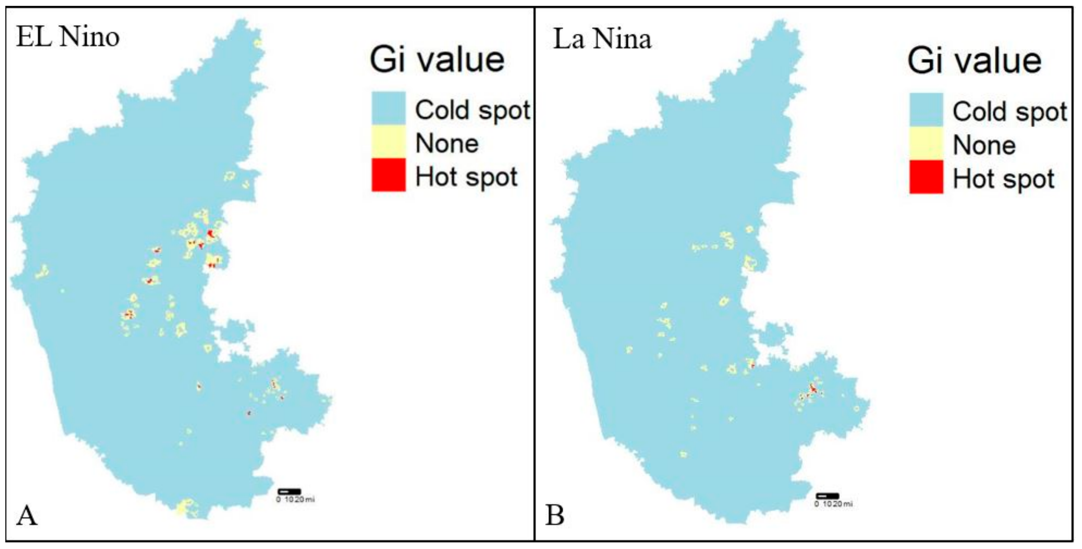
The dataset was verified for the presence of any clusters in the entire dataset prior to hotspot analysis (Getis-Ord Gi*) using a specific method called Moran’s I statistic, a technique for defining global spatial autocorrelation [47]. A prerequisite for hotspot analysis is the presence of clusters within the dataset which gives the output value a z-score, where a high z-score is indicative of a hotspot or cluster. A high z-score for El Niño and La Niña years indicated the presence of hotspots, whereas a negative z-score indicated a cold spot (Figure 4A,B). The Getis-Ord Gi* analysis is being utilized to identify villages/districts with high risks of disease incidence for further analysis and modeling.
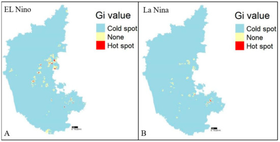
Figure 4.
Hotspot analysis (2004–2019), (A) El Niño years, and (B) La Niña years, respectively.
3.4. Space-Time Cluster Analysis of Anthrax
A discrete Poisson model was used after detecting the existence of a hotspot using Getis-Ord Gi* analysis, and the number of cases of anthrax in each location was assumed to be Poisson distributed. When there are no covariates and the null hypothesis is true, the estimated number of cases in each field is proportional to its population size. The Poisson data was analyzed with purely temporal, purely spatial, and space-time models. The probability function was maximized across all window positions and sizes, and the cluster with the highest likelihood is the most probable and the least likely to have occurred by chance.
Space-time cluster analysis revealed the existence of disease clusters in the central and southeast regions of El Niño and La Niña years from 2004–2019. The spatial variation in El Niño and La Niña years indicated two significant clusters of high risk that were contributing to an increasing pattern in anthrax. From 2004 to 2019, the village-level disease clustering was identified and disease incidence was represented by red colored dots within the significant red circles. This indicates the villages with a high risk of disease incidence, while a pink circle dot represents villages having disease incidence but are not part of significant clusters (Figure 5A,B).
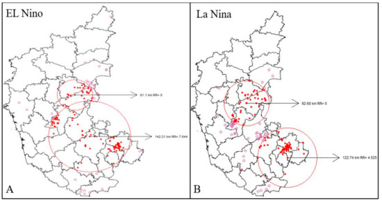
Figure 5.
Space-Time Analysis (2004–2014), (A) El Niño years, and (B) La Niña years, respectively. Where, red spots represent high risk disease incidence and pink spots represent incidence with negligible risk.
3.5. Linear Discriminant Analysis of Anthrax
To identify the ecological, environmental, and other risk factors responsible for the major cluster development after the space-time cluster model identified significant disease clusters. To identify important risk factors (climate, soil profiles, remote sensing, and host) essential for the formation of disease clusters for data at the village level, further, linear discriminant analysis (LDA) was employed. The determining risk factors were then applied to the modeling and prediction of the spatial risks. Table 2 displays the LDA results.

Table 2.
Results of discriminant analysis for El Niño years (2004–2019).
In disease risk modeling, environmental factors that had a p-value of 0.05 or less were found to be significantly correlated with disease occurrence. In El Niño years, the study identified potential risk indicators such as air temperature, wind speed, and potential evaporation rate. The significant risk factors for the La Niña years include air temperature, EVI, NDVI, specific humidity, and wind speed (Table 3). The primary significant risk metrics in the two different groups were placed over the significant clusters (El Niño and La Niña years), which positively influenced the disease incidence.

Table 3.
Results of discriminant analysis for La Niña years (2004–2019).
3.6. Anthrax Risk Assessment and Estimation
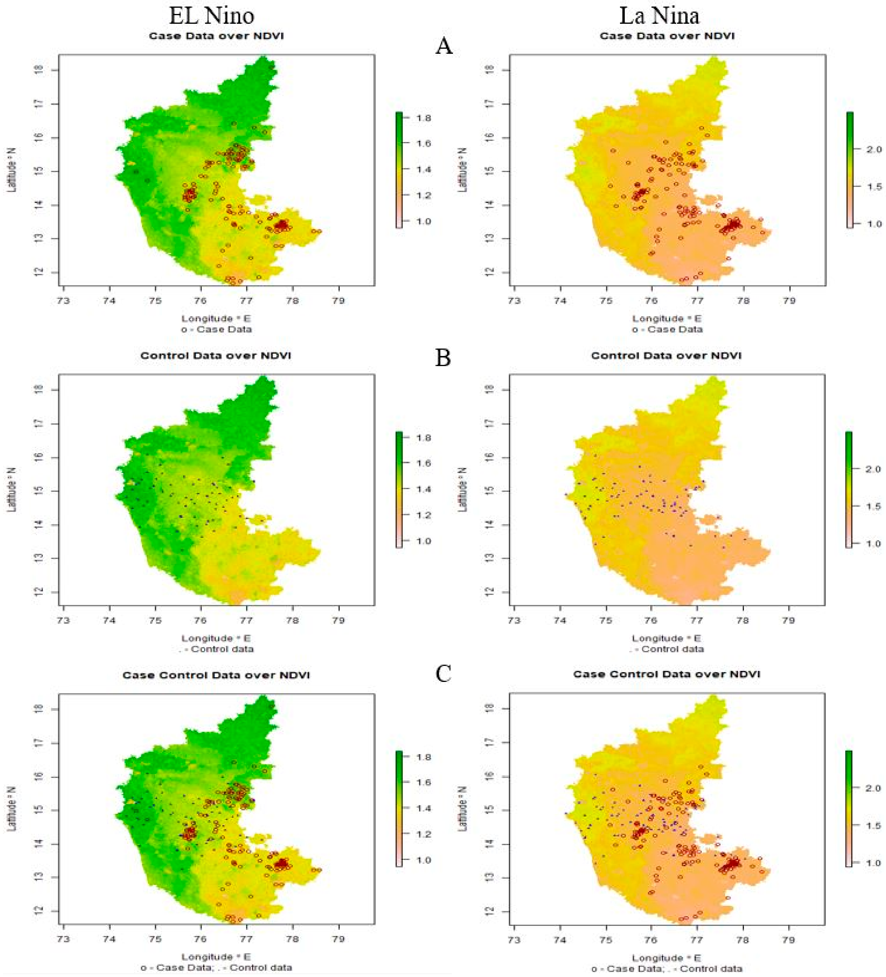
The significant ecological and environmental risk factors identified using LDA were subjected to climate-disease modeling. Maps were generated based on affected (case) and unaffected (control) areas of anthrax (Figure 6). In the map (Figure 6A–C), the case data are represented by red circles, indicating the places having the disease incidences at different thresholds, and the control data are represented by blue dots that indicate the places without incidence of anthrax.

Figure 6.
El Niño and La Niña years’ outbreaks are depicted on a map of Karnataka, respectively. (A) Case data: red-colored circles denote locations where anthrax has been reported, (B) control data: blue-colored dots denote locations where anthrax has not been reported, and (C) case-control data: displays both the existence and absence of anthrax incidence.
Several models using ensemble technology were used for the case-control data. The models’ RF, ADA, and GBM are the most appropriate for both El Niño and La Niña years. The statistically defined evaluation metrics, including ROC, TSS, Cohen’s Kappa, ACCURACY, AUC, F1SCORE, ERROR RATE, and LOGLOSS, were used to determine which models were the best fit. The average score was calculated and recorded for both groups (Table 4A,B).

Table 4.
Model evaluation table (El Niño years). Model evaluation table (La Niña years).
3.7. Anthrax Risk Prediction and Mapping
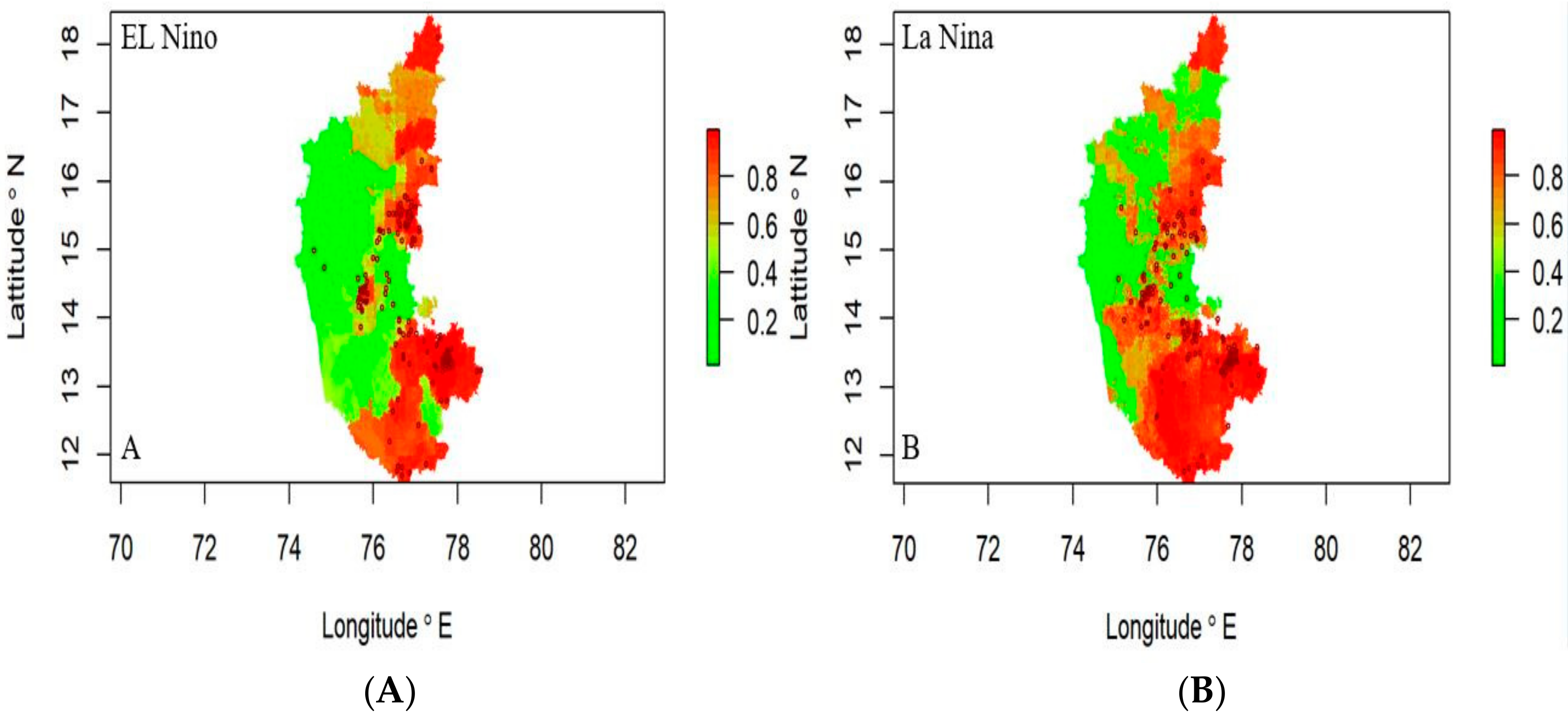
In El Niño years, the disease risk was observed in the northeastern and southern regions, while the western part of the state was not showing any risk (Figure 7A). During La Niña years, the risk was concentrated in the state’s southern, northeastern, and central regions (Figure 7B), indicating severe disease can be expected in these areas.
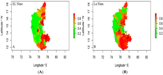
Figure 7.
Anthrax risk prediction map (2004–2019) El Niño years (A) and La Niña years (B), respectively. Where the red spots represent the disease incidence having high risk.
Risk maps offer an enhanced digital platform for a comprehensive view of the likelihood and impact of disease and to develop synergies in a given study area. This increases public awareness, leads the policy makers and planners to take appropriate action that reduces risk to life, and improves risk management governance by highlighting risk management efforts. In this study, a new statistical approach was developed for risk mapping to improve the accuracy of short-term risk prediction. The disease data were modeled with significant predictor variables identified by the LDA function, such as meteorological data, remote sensing data, and host parameters through ensemble machine learning models.
3.8. Estimation of Basic Reproduction Number (R0) of Anthrax
The final step of risk assessment is to estimate the basic reproduction number (R0) and to model R0 with risk already estimated using various risk factors. The result of this stage is more easy to interpret and projectable for the development of suitable preventive actions. The R0 is defined as the exact number of projected secondary cases that one primary case in a susceptible population can generate. This value of R0 has a significant impact on both the daily incidence and the extent of the outbreaks, indicating that more animals would become sick in the foreseeable. The management of diseases in the area can be aided by these insights.
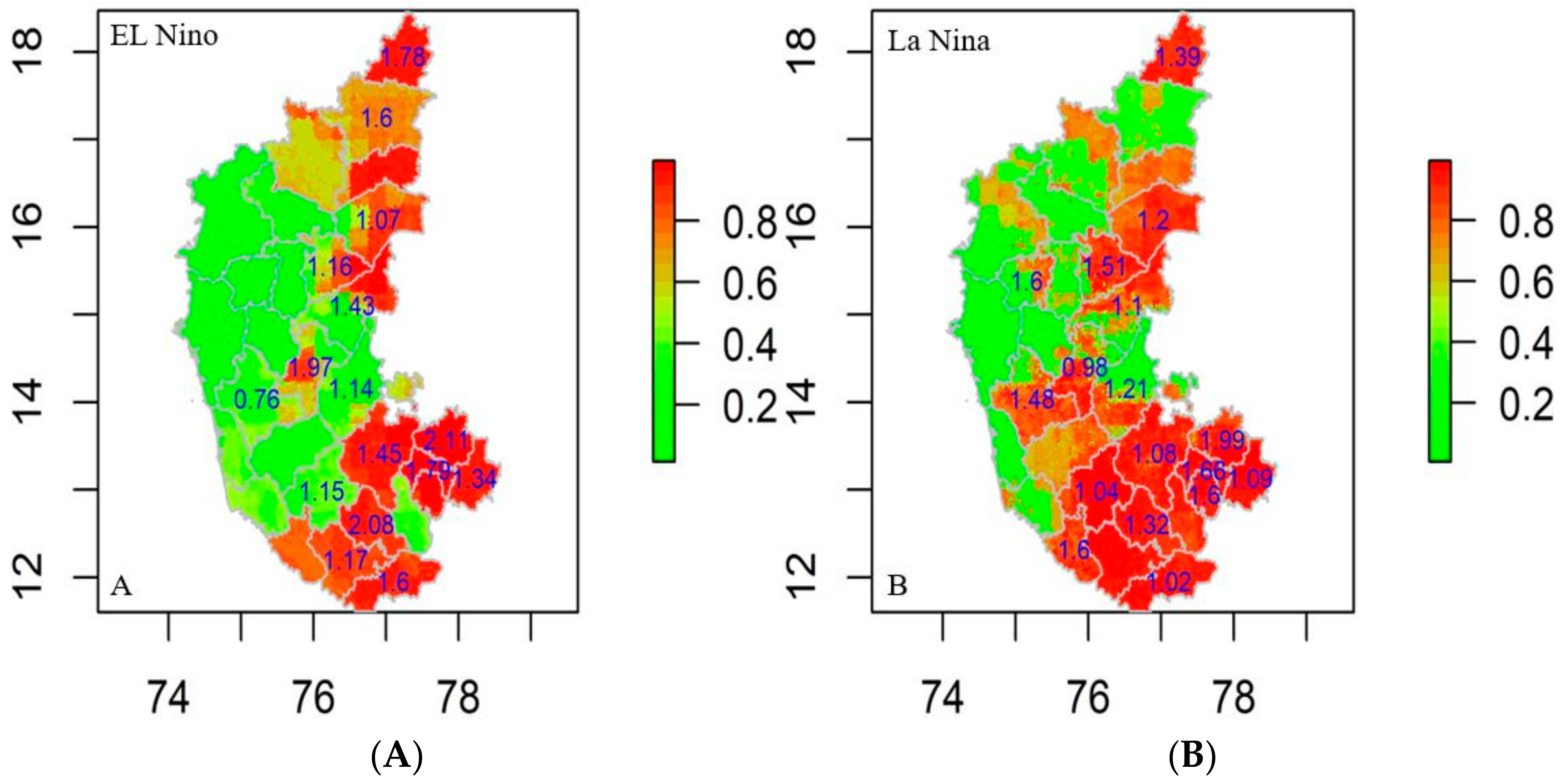
The R0 was estimated for the districts falling in the significantly clustered zone generated by SaTScan and Getis Ord index in the study between 2004 and 2019 based on El Niño and La Niña years. The locations with an R0 value exceeding 1.00 have an increasing trend in disease incidence, complexity, greater risk, and vice versa. The R0 values for El Niño years ranged from 0.76 to 2.11, indicating that the southern and eastern regions are particularly vulnerable to anthrax (Figure 8A). Throughout the La Niña years, the R0 value ranged between 0.98 and 1.99 with high symptom severity in the southern, northeastern, and central regions (Figure 8B). Furthermore, the mobility of infected animals from one location to the other could cause the regions with low R0 values to change to high R0 values in the coming years.
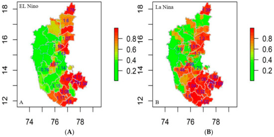
Figure 8.
Anthrax R0 values on risk prediction map district wise (2004–2019) (A) El Niño years and (B) La Niña years, respectively.
4. Discussion
In many scientific and societal domains, the terms early warning and risk prediction are employed to express data on an impending dangerous hazard that enables prompt action to decrease the hazards it poses. Among many other things, early warning or risk prediction is available for natural geophysical, biological, complex socio-political events, industrial, and health threats. A key component of disease risk reduction is an early warning of livestock diseases, which can frequently stop a risk from growing into a veterinary medical crisis by averting the loss of animal wealth and lessening the economic and material effects [48]. This study results in the recognition of machine learning models for early warning of anthrax livestock disease with respect to El Niño and La Niña oscillations and establishes a new approach to the alert system. It may be useful for policymakers and planners to enhance the risk management process. Early recognition of any epidemic animal disease is an important factor that influences the control of disease and helps reduce its socio-economic impact on the country [49]. The persistence of anthrax is strongly correlated with soil pH, as the spore prefers alkaline soil with a relatively high pH for its survival [50]. In the present study, anthrax cases were persistently seen from mildly acidic to mildly alkaline soil PH. Therefore, it can be concluded the pH range of mild acidic to relatively high alkaline is conducive to the survival of the bacterium in soil and the occurrence of the disease. B. anthracis, the responsible bacterium, might cycle between spore germination, vegetative cell outgrowth, and sporulation, which can result in an overall rise in spore counts and subsequent anthrax outbreaks [51]. Additionally, it has been shown that anthrax outbreaks typically happen during the summer season after protracted periods of heavy rain [52]. El Niño is anticipated to cause droughts in India. A prime illustration of this was the drought in 2002, which was accompanied by a strong El Niño and resulted in a more than 19% decrease in Indian monsoon rains out of its long-term average (LPA) [13]. The model analysis depicted the influence of the climate variables on the occurrence of disease. Walsh and his team were among the first to investigate the viability of anthrax along a wide range of northern latitudes, and their study showed an overall risk that, in a broad sense, matched other regional study results regionally and cooperated with earlier reports from Kazakhstan and the United State [8,53]. In our study, we found that the risk parameters, viz., air temperature, soil moisture, NDVI, specific humidity, wind speed, and potential evaporation were significantly influencing the disease occurrence. The research of Margaret Driciru et al. revealed that annual precipitation, exchangeable potassium, annual mean temperature, soil pH, and calcium were the predictor variables favoring the survival and distribution of anthrax spores. Our results were on par with the above result. as the epidemiological triad states the disease can occur only if the environment helps the pathogen travel to the susceptible host [26]. According to a study by Wendy et al., grassland structure, foraging behavior, intake rates, and the chance that forage regions intersect pathogenic accumulations in the environment are all major risk factors for outbreaks. Transmission from soil-borne diseases will also depend on all these factors [54].
Spatial autocorrelation analysis provided a high degree of correlation and clustering of the anthrax outbreaks. Many infectious diseases have distinct regional distributions and seasonal variations, which suggests that they are linked to weather and climate. Studies have demonstrated that temperature, precipitation, and humidity can affect many diseases and vectors’ lifecycles (indirectly and directly through ecological variations), which could have an impact just on the timeliness and severity of disease outbreaks. Numerous studies have found an association between climatic variations and the occurrence of diseases. Early warning or risk prediction is an instrument for communicating information about impending risks to vulnerable livestock populations before a hazardous event occurs, therefore enabling actions to be carried out to mitigate potential harm, viz. outbreak, and sometimes providing an opportunity to prevent the outbreak or incidence from occurring (Climate, ecosystem and infectious diseases; http://www.nap.edu/catlog/10025.html) (accessed on 10 February 2021). In contrast, to date, very little attention is received to the development of early warning or risk prediction worldwide for livestock infectious disease outbreaks. The electronic Disease Early Warning System (eDEWS) is the only system in Yemen that consistently provides data on infectious diseases, although the reliability and prompt service of responses are the major challenges to its performance [49].
Although district-wise early warning of disease occurrence was provided, the lack of awareness, risk identification, and inadequate health care might be responsible for the recurrence of the disease. Machine learning models have been confirmed as successful at mining data from multiple sources to recognize the geographic hotspot and risk vulnerable to outbreaks. Further, it requires contributions from multidisciplinary experts, including meteorologists, epidemiologists, biologists and ecologists, veterinary professionals, public health professionals, policymakers, and local communities on prevention, as well as control of the disease to avoid risk and save the livestock population. This can help with averting economic loss, specifically to protect the livelihood of livestock farmers [16].
The primary goal of early warning or risk prediction is to give dairy farmers and veterinarian medical experts quite enough prior warning of the probable risk of a disease outbreak in a specific region as possible. This will increase the number of feasible alternative responses. The fundamental problem concerning early warning is that reduced predictive accuracy generally results from longer timeframes. Although it is extremely unlikely that a precise disease outbreak forecast would be achieved purely based on environmental observations and host dispersal, this data could be intended to transmit a warning that environmental circumstances are appropriate for disease outbreaks. An early warning system must be considered as an information system designed to aid the relevant regional and national organizations make a decision and also to assist susceptible dairy farmer communities in intervening to reduce the consequences of imminent outbreaks of livestock disease [55]. The attention must not only be on improving livestock disease monitoring and predictions, but also on improving the coordination efforts among the relevant stakeholders, viz., scientific organizations that predict the disease outbreak, the national and local disease management agencies that assess the risk and develop response strategies, disease communication system that facilitate the timely distribution of information impending risk, and risk scenarios or pattern and preparedness measures to vulnerable communities. A key data source for acquiring disease-related information and tracking disease outbreaks is indeed the livestock disease reporting system. ICAR-NIVEDI maintains the database on livestock disease reporting system at village resolution, reported from its own 30 network units in each state, and provides medium-term forecasts that include anthrax as well.
Regardless of the effectiveness of disease and climate modeling techniques, there are still a lot of unanswered questions. The model’s reliability could be increased by emphasizing this limitation and the value of better data. Information processed through early warning would be effective and transformative because of its capability to foresee infectious disease outbreaks and detect a sudden increase in any livestock diseases to potentially stop an epidemic before it spreads. However, under-reporting and non-reporting of disease outbreaks in India is a major threat to the effective implementation of an early warning system.
5. Conclusions
Early warning or risk prediction promotes the systematic epidemiological surveillance activities that are ongoing, the systematic monitoring of climate that uses standardized routines for quality assurance, and helps provide the timely analysis and dissemination of information. The key challenge for an Indian researcher and policy maker is to establish a relationship between El Niño and La Niña with other weather parameters as it is uncertain with an impact example severe drought in India. As per a literature search on this subject, the timing, intensity, and spatial spread of El Niño and La Niña seem to influence Indian monsoon rainfall, but the exact correspondence and its magnitude still appear uncertain. This study tries to explore the relationship of EL Nina and La Niña with other weather parameters by incidence, spread, and prediction of Anthrax diseases in Karnataka. The ecological evidence such as raising air temperature, potential evaporation rate, wind speed, EVI, NDVI, and specific humidity from the present analysis exhibited that anthrax is a significantly major disease in the study area. Prediction of livestock diseases in advance, especially anthrax, is an important task. Machine learning plays a vital role in the prediction of disease risk in the large amount of data annotated with climate and host parameters. The prediction accuracy of machine learning models will be improved by increasing the amount of historical data. Risk prediction and maps developed in the present study serve as beneficial tools for policymakers, veterinarians, and livestock farmers to take necessary healthcare measures against the spread of the disease. In this study, a novel statistical approach for risk mapping improves the accuracy of short-term risk forecasts. Early warning or risk prediction developed with a layer of R0 superimposed on a risk map helps in the preparedness for the disease occurrence, precautionary measures before the spread of the disease, and finding an estimate of the population proportion that must be vaccinated to eliminate the infection from that population.
Author Contributions
Methodology and formal analysis: K.P.S.; conceptualization and data curation: S.B.; writing original draft: S.B.; review and editing: K.P.S., S.P., C.S., S.P.K. and R.G.A.; formatting and editing: U.B.I. and B.A.P.; supervision: P.T.S., C.A.C. and R.G.A.; visualization: M.K. All authors have read and agreed to the published version of the manuscript.
Funding
This research received no external funding.
Institutional Review Board Statement
This study does not involve any animals or humans directly and only data on some outbreaks were obtained, hence ethical approval was not necessary.
Informed Consent Statement
Not applicable.
Data Availability Statement
Available on request.
Acknowledgments
Authors thank the Dept. of Animal Husbandry and Veterinary Services, Government of Karnataka for sharing the data on the prevalence of anthrax. We are also grateful to DG and DDG (AS), ICAR and Director, ICAR-NIVEDI for their constant support, guidance and necessary assistance during the study.
Conflicts of Interest
The authors have no conflict of interest.
References
- Serkan, O.; Selcen, O.; Serhan, S. Anthrax—An overview. Med. Sci. Monit. 2003, 9, 276–283. [Google Scholar]
- Jayachandran, R. Anthrax: Biology of Bacillus anthracis. Curr. Sci. 2002, 82, 1220–1226. [Google Scholar]
- Jocelyn, M.; Larissa, L.; Alim, A.; Yerlan, P.; Mathew, V.E.; Jason, K.B. Ecological Niche Modelling of the Bacillus anthracis A1.a sub-lineage in Kazakhstan. BMC Ecol. 2011, 11, 32. [Google Scholar]
- Turnbull, P.C.B. Guidelines for the Surveillance and Control of Anthrax in Humans and Animals; WHO/EMC/ZDI/98.6, Wiltshire SP4 0JG; World Health Organization: Geneva, Switzerland, 1998. [Google Scholar]
- Gombe, N.T.; Nkomo, B.M.M.; Chadambuka, A.; Shambira, G.; Tshimanga, M. Risk factors for contracting anthrax in Kuwirirana ward, Gokwe North, Zimbabwe. Afr. Health Sci. 2010, 10, 159–164. [Google Scholar]
- Madeleine, C.T.; Angel, G.M.; Remi, C.; Joy, S.G. Climate drivers of vector-borne diseases in Africa and their relevance to control programmes. Infect. Dis. Poverty 2018, 7, 81. [Google Scholar]
- Myers, M.F.; Rogers, D.J.; Cox, J.; Flahault, A.; Hay, S.I. Forecasting Disease Risk for Increased Epidemic Preparedness in Public. Health Adv. Parasitol. 2000, 47, 309–330. [Google Scholar]
- Michael, G.W.; de Smalen, A.W.; Siobhan, M.M. Climatic influence on anthrax suitability in warming northern latitudes. Sci. Rep. 2018, 8, 9269. [Google Scholar]
- Troccoli, A. Review Seasonal climate forecasting. Metrol. Appl. 2010, 17, 251–268. [Google Scholar] [CrossRef]
- Kriss, A.B.; Paul, P.A.; Madden, L.V. Variability in Fusarium Head Blight Epidemics in Relation to Global Climate Fluctuations as Represented by the El Niño-Southern Oscillation and Other Atmospheric Patterns. Ecol. Epidemiol. 2012, 55, 64. [Google Scholar] [CrossRef]
- Malay, P.; Poonam, S.; Kumar, G.; Ojha, V.P.; Dhiman, R.C. El Niño Southern Oscillation as an early warning tool for dengue outbreak in India. BMC Public Health 2020, 20, 1498. [Google Scholar]
- Cane, M.A. The evolution of El Niño, past and future. Earth Planet. Sci. Lett. 2005, 230, 227–240. [Google Scholar] [CrossRef]
- Saini, S.; Ashok, G. El Niño and Indian Droughts: A Scoping Exercise; No. 276, Working Paper; Indian Council for Research on International Economic Relations (ICRIER): New Delhi, Indian, 2014. [Google Scholar]
- Cherian, S.; Sridhara, S.; Manoj, K.N.; Gopakkali, P.; Ramesh, N.; Alrajhi, A.A.; Dewidar, A.Z.; Mattar, M.A. Impact of El Niño Southern Oscillation on Rainfall and Rice Production: A Micro-Level Analysis. Agronomy 2021, 11, 1021. [Google Scholar] [CrossRef]
- Anna, M.S.; Rachel, L. Climate and Non-Climate Drivers of Dengue Epidemics in Southern Coastal Ecuador. Am. J. Trop. Med. Hyg. 2013, 88, 971–981. [Google Scholar]
- Pinto, J.; Bonacic, C.; Hamilton-West, C.; Romero, J.; Lubroth, J. Climate change and animal diseases in South America. Rev. Sci. Tech. 2008, 27, 599–613. [Google Scholar] [CrossRef] [PubMed]
- Debashish, D. Machine learning algorithms for disease prediction: A methodological Review in Biomedical. In Proceedings of the 3rd Global Conference on Computing and Media Technology, Kuala Lumpur, Malaysia, 17–18 July 2019. [Google Scholar]
- Carella, E.; Orusa, T.; Viani, A.; Meloni, D.; Borgogno-Mondino, E.; Orusa, R. An Integrated, Tentative Remote-Sensing Approach Based on NDVI Entropy to Model Canine Distemper Virus in Wildlife and to Prompt Science-Based Management Policies. Animals 2022, 12, 1049. [Google Scholar] [CrossRef]
- Orusa, T.; Mondino, E.B. Exploring Short-term climate change effects on rangelands and broad-leaved forests by free satellite data in Aosta Valley (Northwest Italy). Climate 2021, 9, 47. [Google Scholar] [CrossRef]
- Orusa, T.; Orusa, R.; Viani, A.; Carella, E.; Mondino, E.B. Geomatics and EO data to support wildlife diseases assessment at landscape level: A pilot experience to map infectious keratoconjunctivitis in chamois and phenological trends in Aosta Valley (NW Italy). Remote Sens. 2020, 12, 3542. [Google Scholar] [CrossRef]
- Ward, M.M. Estimating disease prevalence and incidence using administrative data: Some assembly required. J. Rheumatol. 2013, 40, 1241–1243. [Google Scholar] [CrossRef]
- Ranganath, R.N.; Jayaraman, V.; Roy, P.S. Remote sensing applications: An overview. Curr. Sci. 2007, 93, 1747–1766. [Google Scholar]
- Suma, A.P.; Suresh, K.P.; Gajendragad, M.R.; Kavya, B.A. Forecasting Anthrax in Livestock in Karnataka State using Remote Sensing and Climatic Variables. Int. J. Sci. Res. 2015, 6, 1891–1897. [Google Scholar]
- Justice, C.O.; Townshend, J.R.G.; Vermote, E.F.; Masuoka, E.; Wolf, R.E.; Saleous, N.; Roy, D.P.; Morisette, J.T. An overview of MODIS Land data processing and product status. Remote Sens. Environ. 2002, 83, 3–15. [Google Scholar] [CrossRef]
- Hay, S.I.; Tatem, A.J.; Graham, A.J.; Goetz, S.J.; Rogers, D.J. Global Environmental Data for Mapping Infectious Disease Distribution. Adv Parasitol. 2006, 62, 37–77. [Google Scholar] [PubMed]
- Margaret, D.; Rwego, I.B.; Ndimuligo, S.A.; Travis, D.A.; Mwakapeje, E.R.; Craft, M.; Asiimwe, B.; Alvarez, J.; Ayebare, S.; Pelican, K. Environmental determinants influencing anthrax distribution in Queen Elizabeth Protected Area, Western Uganda. PLoS ONE 2020, 15, e0237223. [Google Scholar]
- Horvath, D.J.; Reid, R.L. Indirect effects of soil and water on Animal health. Sci. Total Environ. 1984, 34, 143–156. [Google Scholar] [CrossRef]
- Lawrence, N.K.; Adamson, S.M.; Christopher, C.A.; Immo, K. Modelling the effect of malaria endemicity on spatial variations in childhood fever, diarrhoea and pneumonia in Malawi. Int. J. Health Geogr. 2007, 6, 33. [Google Scholar]
- Songchitruksa, P.; Zeng, X. Getis–Ord Spatial Statistics to Identify Hot Spots by Using Incident Management Data. Transp. Res. Rec. 2010, 2165, 42–51. [Google Scholar] [CrossRef]
- Tobler, W.R. A Computer movie simulating urban growth in the detroit region. Econ. Geogr. 1970, 46, 234–240. [Google Scholar] [CrossRef]
- Michael, J.; Sara, G.; Caitlin, K. Spatial Modeling in Environmental and Public Health Research. Int. J. Environ. Res. Public Health. 2010, 7, 1302–1329. [Google Scholar]
- Muluken, A.; Abera, K.; Alemayehu, W.; Bagtzoglou, A.C. Childhood Diarrhea Exhibits Spatiotemporal Variation in Northwest Ethiopia: A SaTScan Spatial Statistical Analysis. PLoS ONE 2015, 10, e0144690. [Google Scholar]
- Marlize, C.; Michael, C.; Aaron, M.M.; Gerdalize, K.; Maureen, C.; David, N.D. Using the SaTScan method to detect local malaria clusters for guiding malaria control programmes. Malar J. 2009, 8, 68. [Google Scholar]
- Shahera, B.; Wenbiao, H.; Cameron, H.; Yuming, G.; Mohammad, Z.I.; Shilu, T. Space-time clusters of dengue fever in Bangladesh. Trop. Med. Int. Health 2012, 17, 1086–1091. [Google Scholar]
- Izenman, A.J. Linear Discriminant Analysis. In Springer Texts in Statistics; Springer: Berlin/Heidelberg, Germany, 2013. [Google Scholar]
- Pankaj, M.; Ching-Hao, W.; Alexandre Day, G.R.; Clint, R.; Marin, B.; Charles, K.F.; David, J.S. A high-bias, low-variance introduction to Machine Learning for physicists. Phys. Rep. 2019, 810, 1–124. [Google Scholar]
- Omri, A.; Asaf, T.; Ronen, K. Assessing the accuracy of species distribution models: Prevalence, kappa and the true skill statistic (TSS). J. Appl. 2006, 43, 1223–1232. [Google Scholar]
- Andrius, V.; Emma, G.; Ellen, P.; Alexander, J.C. Machine learning algorithm validation with a limited sample size. PLoS ONE 2019, 14, e0224365. [Google Scholar]
- Johnson, K.; Vinay, K.K.; Phridviraj, M.S.B.; Shaik, R. Reducing Overfitting Problem in Machine Learning Using Novel L1/4 Regularization Method. In Proceedings of the Fourth International Conference on Trends in Electronics and Informatics, Tirunelveli, India, 16–18 April 2020. [Google Scholar]
- Jake, L.; Martin, K.; Naomi, A. Model selection and overfitting. Nat. Methods 2016, 13, 703–704. [Google Scholar]
- Farzin, S.; Lalit, K.; Mohsen, A. Assessing Accuracy Methods of Species Distribution Models: AUC, Specificity, Sensitivity and the True Skill Statistic. Glob. J. 2018, 18, 1–13. [Google Scholar]
- Ferri, C.; Hernández-Orallo, J.; Modroiu, R. An experimental comparison of performance measures for classification. Pattern Recognit. Lett. 2009, 30, 27–38. [Google Scholar] [CrossRef]
- Li, Y.; Wang, L.-W.; Peng, Z.-H.; Shen, H.-B. Basic reproduction number and predicted trends of coronavirus disease 2019 epidemic in the mainland of China. Infect. Dis. Poverty. 2020, 9, 1–13. [Google Scholar] [CrossRef]
- Mahmud, R.; Patwari, H.A.F. Estimation of the Basic Reproduction Number of SARS-CoV-2 in Bangladesh Using Exponential Growth Method. Infect Dis. Poverty 2020, 9, 94. [Google Scholar]
- Froda, S.; Leduc, H. Estimating the basic reproduction number from surveillance data on past epidemics. Math. Biosci. 2014, 256, 89–101. [Google Scholar] [CrossRef]
- Obadia, T.; Haneef, R.; Boëlle, P.-Y. The R0 package: A toolbox to estimate reproduction numbers for epidemic outbreaks. BMC Med. Inform. Decis. Mak. 2012, 12, 147. [Google Scholar] [CrossRef] [PubMed]
- Xiong, Y.; Bingham, D.; Braun, W.J.; Hu, X.J. Moran’s I statistic-based nonparametric test with spatio-temporal observations. J. Nonparametric Stat. 2019, 31, 244–267. [Google Scholar] [CrossRef]
- Hamid, R.K.; Seyed, H.H.; Mehrdad, F.; Mohammad, A.H.; Nasir, A. Early warning system models and components in emergency and disaster: A systematic literature review protocol. Syst. Rev. 2019, 8, 315. [Google Scholar]
- Fekri, D.; Kamran, A.; Claudia, B.; Claire, J.S.; Ali, A.; Albrecht, J. Assessment of electronic disease early warning system for improved disease surveillance and outbreak response in Yemen. BMC Public Health 2020, 20, 1422. [Google Scholar]
- Ian, T.K.; Lile, M.; Nikoloz, T.; Julietta, M.; Lela, B.; Paata, I.; Shota, T.; Jason, K.B. Evidence of Local Persistence of Human Anthrax in the Country of Georgia Associated with Environmental and Anthropogenic Factors. PLoS Negl. Trop. Dis. 2013, 7, 9. [Google Scholar]
- Sean, B.; Thuillier, G.; Barlier, F. The DTM-2000 empirical thermosphere model with new data assimilation and constraints at lower boundary: Accuracy and properties. J. Atmos. Sol.-Terr. Phys. 2003, 65, 1053–1070. [Google Scholar]
- Dragon, D.C.; Rennie, R.P. The ecology of anthrax spores: Tough but not invincible. Can. Vet. J. 1995, 36, 295–301. [Google Scholar]
- Gunaseelan, L.; Rishikesavan, R.; Adarsh, T.; Baskar, R.; Hamilton, E.; Kaneene, J.B. Temporal and geographical distribution of animal anthrax in Tamil Nadu state, India. Tamilnadu J. Vet. Anim. Sci. 2011, 7, 277–284. [Google Scholar]
- Turner, W.C.; Imologhome, P.; Havarua, Z.; Kaaya, G.P.; Mfune, J.K.E.; Mpofu, I.D.T.; Getz, W.M. Soil ingestion, nutrition and the seasonality of anthrax in herbivores of Etosha National Park. Ecosphere 2013, 4, 1–19. [Google Scholar] [CrossRef]
- Bylaiah, S.; Shedole, S.; Suresh, K.P.; Gowda, L.; Shivananda, B.; Shivamallu, C.; Patil, S.S. Disease Prediction Model to Assess the Impact of Changes in Precipitation Level on the Risk of Anthrax Infectiousness among the Livestock Hosts in Karnataka, India. Int. J. Spec. Educ. 2022, 37, 711–727. [Google Scholar]
Publisher’s Note: MDPI stays neutral with regard to jurisdictional claims in published maps and institutional affiliations. |
© 2022 by the authors. Licensee MDPI, Basel, Switzerland. This article is an open access article distributed under the terms and conditions of the Creative Commons Attribution (CC BY) license (https://creativecommons.org/licenses/by/4.0/).

